Abstract
Accurate reservoir identification from well-logging data is crucial for hydrocarbon exploration, yet challenges persist due to a series of factors, including limitations such as low efficiency and subjectivity of manual processing for massive datasets, as well as class imbalance and its impact on machine learning model training. This study develops an intelligent identification model using a Convolutional Neural Network (CNN) enhanced with Focal Loss, applied to real well-logging data from the Chang 8 Member of the Yanchang Formation in the Jiyuan Oilfield, Ordos Basin. A well-based data partitioning strategy is adopted to ensure the model’s generalization ability to new wells, avoiding the overoptimistic performance associated with random sample splitting. Experimental results demonstrate that the proposed model achieves an Accuracy of 84% and a Recall of 83% for oil-bearing layers. In comparison, the Random Forest model achieves a lower Recall of 56% for oil-bearing layers, and the CNN-LSTM model achieves 77%. The key influential well-logging parameters identified are bulk density (DEN), spontaneous potential (SP), true resistivity (RT), and natural gamma ray (GR). The findings confirm that the Focal Loss-enhanced CNN effectively mitigates class imbalance issues and provides a reliable, automated method for reservoir identification, offering significant practical value for the secondary interpretation of well logs in similar tight sandstone reservoirs.
1. Introduction
Oil and gas exploration and development play a crucial role in ensuring energy security and promoting economic growth. However, the accurate identification and evaluation of reservoirs are among the core challenges in hydrocarbon exploration [1]. Well logging, as the most direct and commonly used geophysical exploration method, provides continuous information on subsurface lithology, physical properties, and fluid characteristics, thereby offering reliable data support for the identification and classification of oil and gas reservoirs. Effectively utilizing well-logging data to accurately identify reservoirs under complex geological conditions is key to improving the efficiency of exploration and development [2].
Traditional reservoir interpretation methods primarily rely on geologists’ empirical judgment, as well as on chart-based or statistical techniques derived from physical equations [3,4,5,6]. However, as exploration efforts increasingly focus on unconventional reservoirs, traditional identification approaches face significant challenges due to geological complexity and reservoir heterogeneity—such as low porosity, low permeability, and complex fluid distributions. For example, when well-logging response differences are subtle, methods based on resistivity interpretation and empirical crossplot analysis often struggle to distinguish gas-bearing layers from water-bearing ones. Similarly, techniques that depend on rock physics models or a limited set of simple geophysical well-logging parameters (e.g., resistivity and porosity) tend to be inadequate under the complex geological conditions typical of tight oil and gas reservoirs [7,8,9]. In addition, statistical methods that rely on historical production data or empirical models, though computationally efficient, are constrained by their dependence on linear assumptions and low-dimensional parameter interactions [10,11]. Therefore, there is an urgent need to develop advanced and robust methods capable of effectively tackling the inherent nonlinearity and high-dimensional characteristics involved in tight reservoir evaluation.
Currently, data-driven machine learning methods, owing to their excellent ability to explore nonlinear relationships between well-logging responses, represent a promising breakthrough in addressing this issue and have gained favor among many scholars. Cheng Chao et al. [12] compared the fluid property identification results of decision trees, neural networks, extreme gradient boosting (XGBOOST), and other machine learning algorithms with those of traditional identification methods for low-resistivity oil reservoirs. The machine learning algorithm results outperformed those of the graphical methods, with XGBOOST showing the best performance. Zhang Junlong et al. [13] conducted a lithology identification study based on well-logging data from the Junggar Basin using machine learning techniques. The results demonstrated that ensemble methods (XGBoost and RF) achieved an overall classification accuracy of 0.88 when distinguishing among mudstone, sandstone, and sandy conglomerate. Zhou Xinmao et al. [14] used an SVM for fluid identification in thin reservoirs, achieving an identification accuracy of 85.7% by introducing kernel functions and establishing a thin reservoir prediction model. Although these traditional machine learning methods offer good interpretability and fast training speed, they still have limitations in feature extraction and modeling complex data structures, which hinder their ability to achieve the high accuracy and strong robustness required for tight reservoir identification [15]. As a result, an increasing number of researchers have turned to deep learning techniques to address these challenges.
Compared with traditional machine learning, deep learning—particularly convolutional neural networks (CNNs)—offers enhanced capabilities for the autonomous extraction of high-dimensional features. Liu Mingliang et al. [16] conducted a study on 3D seismic facies classification, showing that when sufficient well data is available, a supervised CNN can accurately reconstruct a three-dimensional facies model. Qi Ming et al. [17] successfully introduced CNNs to construct a diagenetic facies identification model based on well-logging data, and the predicted diagenetic facies of tight oil reservoirs exhibited a high degree of consistency with thin section analyses of core samples, providing crucial technical support for accurate reservoir evaluation. Luo Gang et al. [18] combined CNNs with long short-term memory (LSTM) networks to capture both spatial and temporal features of well-logging data, substantially improving the accuracy of fluid identification in tight sandstone reservoirs. Shi Yu et al. [19] applied a residual convolutional neural network (ResCNN) to training on well-logging data and achieved a high lithology classification accuracy of 93%, highlighting the powerful feature extraction ability of CNNs. Collectively, these studies confirm that CNNs are particularly well-suited for learning and distinguishing subtle patterns in well-logging data related to lithology and fluid properties, thereby significantly enhancing classification accuracy.
However, the performance of deep learning models in processing geophysical data is often severely constrained by the class imbalance problem. To address this pervasive issue, recent studies have proposed solutions from both data-level and algorithm-level perspectives. At the algorithm level, Farahnakian et al. [20] successfully employed a two-stage framework to handle extreme imbalance in mineral prospectivity mapping. Banar and Mohammadi [21] utilized deep reinforcement learning to dynamically assign rewards and penalties, thereby enhancing sensitivity to rare seismic events. On the data side, generative AI such as diffusion models has been adopted by researchers to synthesize high-quality minority-class samples for digital rock images [22]. In well-logging interpretation, Li et al. [23] effectively improved the identification of rare lithofacies by integrating Borderline SMOTE (BSMOTE) with a hybrid CNN-GRU model. Particularly relevant to this work, prior research specifically modified Focal Loss for 3D mineral prospectivity modeling, proposing a Class-Balanced Focal Loss (CBFL) and demonstrating its superiority [24]. These advances confirm that designing adaptive loss functions tailored to specific geoscientific data characteristics is a viable and effective pathway to mitigate the class imbalance challenge.
In addition, existing studies often construct training and validation sets by randomly partitioning samples when training machine learning models. This approach may result in samples from the same well appearing in both the training and validation sets, leading to an overestimation of model performance and preventing the evaluation results from accurately reflecting the model’s generalization ability to new wells.
In summary, inspired by the aforementioned research and addressing its existing limitations, this study focuses on the tight sandstone reservoirs of the Chang 8 Member in the Jiyuan Oilfield, Ordos Basin, to conduct research on intelligent reservoir identification. Its core innovations are reflected in three aspects:
- Proposing a well-based data partitioning strategy to avoid sample leakage and more authentically evaluate the model’s generalization ability (consistent with the other two innovations in temporal logic);
- Validating the exceptional effectiveness of Focal Loss in addressing class imbalance in this domain;
- Providing interpretable physical insights through mutual information analysis.
The aim is to develop a feasible and efficient intelligent reservoir identification method that overcomes the limitations of traditional well-logging interpretation and provides valuable references for similar studies in other regions.
2. Regional Geological Setting
The Ordos Basin, located in central China, is the country’s second-largest inland sedimentary basin. Tectonically situated on the western margin of the North China Block, the basin is characterized by a large, asymmetric syncline with a broad eastern flank and a steep western flank. The basin comprises several tectonic units, with the Yishan slope being the primary unit for hydrocarbon accumulation, hosting over 90% of the discovered reserves. This study focuses on the Jiyuan Oilfield, located in the central-western part of the Ordos Basin (Figure 1a,b).
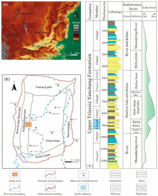
Figure 1.
(a) Location of the Ordos Basin; (b) substructural units and location map of the Jiyuan area in the Ordos Basin; (c) comprehensive stratigraphic column (modified from He Taping et al. [25]).
The primary target reservoir is the Chang 8 member of the Upper Triassic Yanchang Formation (T3y), which was deposited in fluvio-deltaic and lacustrine depositional environments [26,27]. Vertically, the Yanchang Formation is subdivided into ten members: Chang 10, Chang 9, Chang 8, Chang 7, Chang 6, Chang 4 + 5 (an integrated unit of Chang 4 and Chang 5, grouped for their consistent lithology and depositional settings in the Ordos Basin), Chang 3, Chang 2, and Chang 1 (Figure 1c). The Chang 8 member, with a thickness of 75–95 m, is composed predominantly of underwater distributary channel sandstones and can be further subdivided into two sub-members, Chang 81 and Chang 82 (Table 1). The reservoirs in this region are typical tight sandstones, exhibiting low permeability, low pressure, and low abundance (“three-low” characteristics), which pose significant challenges for accurate identification and evaluation.

Table 1.
Chang 8 stratigraphic table of the Yanchang Formation in the Jiyuan area.
The geological characteristics of the Chang 8 tight sandstone reservoirs directly informed the methodological design of this study. The reservoir heterogeneity, subtle differences in well-logging responses between fluid types, and the inherent class imbalance motivated the adoption of a CNN architecture for local pattern extraction and the integration of Focal Loss to mitigate the bias caused by imbalanced sample distribution. The well-based data partitioning strategy was also designed to respect the geological independence between different well locations, ensuring a realistic assessment of model generalization in such a complex depositional system.
3. Materials and Methods
3.1. Well Log Data Collection and Feature Selection
The research dataset originates from a genuine well-logging dataset of the Chang 8 oil layer group in the Triassic Yanchang Formation (T3y) within the Jiyuan area of the Ordos Basin (Figure 2).
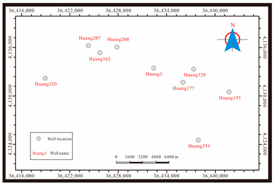
Figure 2.
Well locations in the study area. Note: The horizontal and vertical coordinates in this map refer to the Gauss–Krüger plane rectangular coordinates (unit: meter).
To comprehensively characterize reservoir lithology, pore structure, and fluid properties, nine commonly used well-logging curves were selected as input features. These include acoustic time difference (AC), compensated neutron log (CNL), natural gamma ray (GR), spontaneous potential (SP), true resistivity (RT), bulk density (DEN), and caliper log (CAL), among others. These parameters collectively capture reservoir porosity, hydrogen content, lithological variation, permeability, and fluid characteristics, offering multidimensional and complementary information for the model. In particular, parameters such as RT, CNL and DEN exhibit significant variations across different fluid types, thereby enhancing classification discriminability.
This dataset comprises data from 9 wells, encompassing a total of 6409 samples with a sampling interval of 0.125 m. All data were initially labeled by experienced technical personnel and subsequently validated by multiple domain experts, ensuring the reliability and scientific rigor of the dataset. This high-quality dataset provides a solid foundation for model development and evaluation. Figure 3, Figure 4, Figure 5, Figure 6, Figure 7, Figure 8 and Figure 9 show boxplots of the data distributions for different well-logging response parameters. Figure 10 shows the data distribution characteristics of well-logging response parameters. Table 2 presents the statistical characteristics of the different well-logging response parameters. To assess redundancy and complementarity among the seven input features, we calculated the Pearson correlation coefficient matrix (Figure 11).
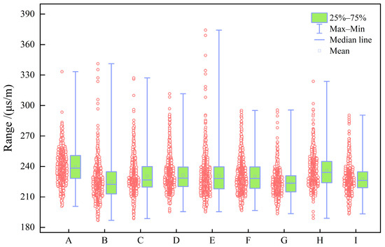
Figure 3.
Box plot of AC (μs/m).
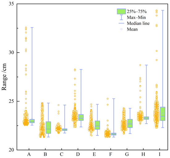
Figure 4.
Box plot of CAL (cm).
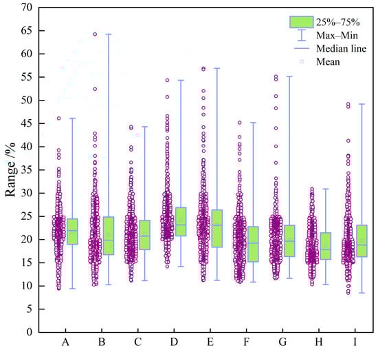
Figure 5.
Box plot of CNL (%).
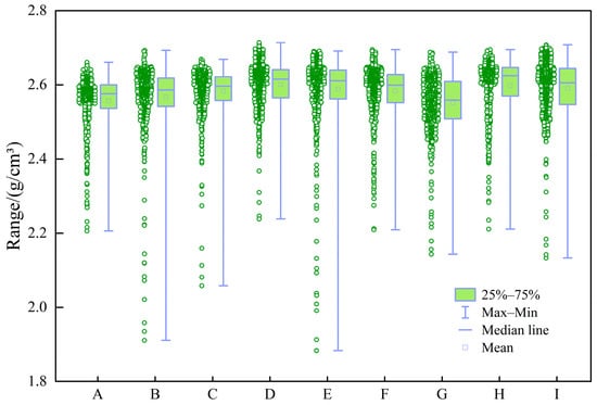
Figure 6.
Box plot of DEN (g/cm3).
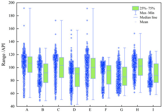
Figure 7.
Box plot of GR (API).
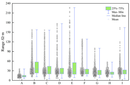
Figure 8.
Box of RT (Ω·m).
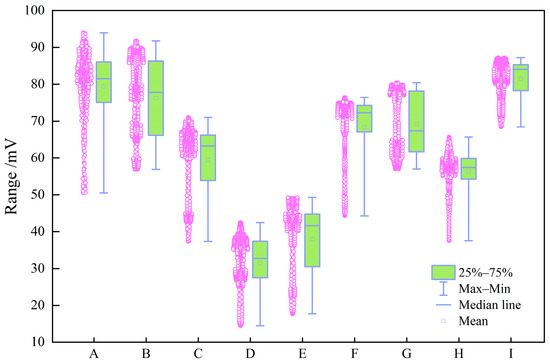
Figure 9.
Box plot of SP (mV).
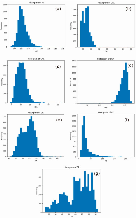
Figure 10.
Data distribution characteristics of well-logging response parameters: (a) AC; (b) CAL; (c) CNL; (d) DEN; (e) GR; (f) RT; (g) SP.
Table 2.
Statistical characteristics of well-logging response parameters.
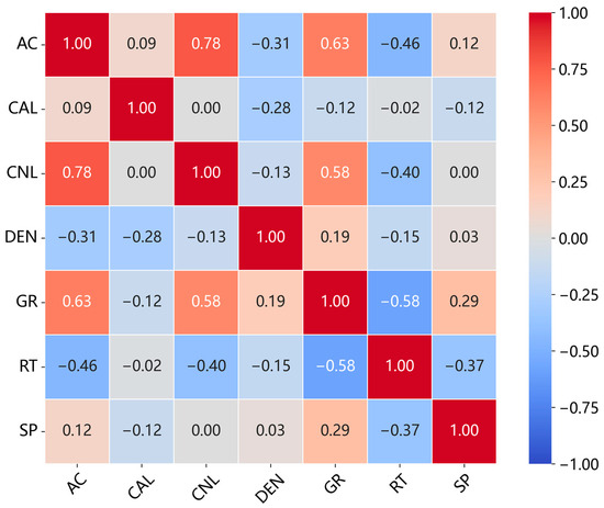
Figure 11.
Pearson correlation matrix of the seven well-logging parameters.
The box plots in Figure 3, Figure 4, Figure 5, Figure 6, Figure 7, Figure 8 and Figure 9 indicate that individual well-logging parameters exhibit considerable overlap among different reservoir types, with no single parameter providing a clear discriminative threshold. At the same time, variations in median values, interquartile ranges, and outlier distributions suggest that each parameter contains partial discriminative information. The data distribution characteristics in Figure 10 indicate that the data require appropriate preprocessing before being input into the model so as to reduce the impact of skewed distribution on model training. Figure 11 indicates that the well-logging parameters exhibit moderate correlations resulting from shared geological and petrophysical controls while still preserving substantial complementary information, demonstrating that multi-parameter integration is both necessary and reasonable and that no severe feature redundancy exists among the input well logs.
The model outputs include three reservoir types: oil-bearing layer, water layer, and non-reservoir. Importantly, in this regional dataset, the non-reservoir accounts for 83%, the oil-bearing layer accounts for 15%, and the water layer accounts for 2%. Clearly, the data distribution is imbalanced (Figure 12).
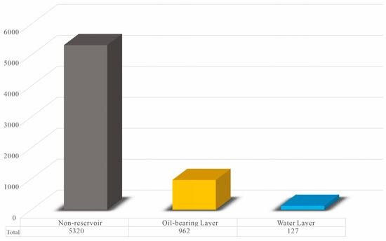
Figure 12.
Reservoir type sample statistics.
3.2. Data Preprocessing and Outlier Handling
Prior to model training, we implemented a rigorous data cleaning procedure based on physically plausible ranges derived from petrophysical principles and regional geological characteristics of the Chang 8 Formation in the Ordos Basin. These thresholds were established through consultation with domain experts and analysis of core-log integration studies in the Jiyuan area:
- AC: 180–350 μs/m (excluding extreme values caused by borehole collapse or instrument failure);
- CAL: 20–26 cm (excluding severe borehole washout or collapse);
- CNL: 8–30% (consistent with the neutron response characteristics of sandstone reservoirs);
- DEN: 2.4–2.8 g/cm3 (typical density range of tight sandstones);
- GR: 40–150 API (excluding ultra-shaly or radioactive mineral anomalies);
- RT: 4.5–200 Ω·m (excluding extreme high resistivity caused by instrument drift);
- SP: 10–95 mV (excluding extreme electrochemical anomalies).
Based on the above ranges, a total of 187 abnormal samples (accounting for 2.92% of the original samples) were removed. The changes in the statistical characteristics of the processed data are shown in Table 3. It can be seen that the standard deviation (Std) of each parameter has decreased, the data distribution is more concentrated, and it is consistent with the geological laws of well-logging responses in the study area.
Table 3.
Changes in statistical characteristics of well-logging parameters after outlier handling.
All well-logging parameters were then standardized using Z-score normalization, which transforms each feature into a normal distribution with a mean of 0 and a standard deviation of 1 (Equation (1)). This procedure eliminates the effects of differing units and scales among features, ensuring that all variables contribute equally during model training and preventing features with larger numerical ranges from dominating the learning process.
where denotes the actual well-logging data, represents its mean, and represents its standard deviation.
3.3. Dataset Splitting
To establish a predictive model with strong generalization capabilities, it is common practice to partition the dataset into training and validation data. Various methods can be employed for dataset partitioning, including random splitting based on proportions or grouping by data characteristics. In the research task of this paper, if the dataset is randomly divided in proportion, it can improve the generalization performance and identification accuracy of the model. However, this approach overlooks the independence between different wells, which can lead to severe overfitting and prevent the model from accurately reflecting its generalization capability to new wells. Therefore, in this research task, the traditional proportional partitioning principle must yield to more critical geological logic.
Therefore, this study adopts a well-based partitioning strategy. All wells are uniformly distributed in the Huang3 Block in the western part of the Jiyuan Oilfield, where no large-scale structures are developed, and the geological structure is simple and homogeneous. The partitioning is mainly based on two considerations: first, the data characteristics of the wells should cover different sedimentary microfacies in the study area; second, the ratio of training to validation samples should be maintained at 7:3. This ensures that the model learns regionally representative features and enables the evaluation of its generalization ability to new wells. Specifically, data from 9 wells are used: the training set includes Well Huang120, Well Huang193, Well Huang207, Well Huang208, Well Huang254, and Well Huang320; the validation set includes Well Huang3, Well Huang162, and Well Huang177.
3.4. Model Architecture
3.4.1. Convolutional Neural Network
In this study, we utilize a convolutional neural network (CNN) to extract the vertical variation features of well-logging data. Essentially, well log curves are continuous sequences sampled in depth order. By sliding convolutional kernels along the vertical sequence of well-logging data, the CNN can effectively capture local feature patterns corresponding to depth variations while preserving the correlations between adjacent layers. This characteristic makes CNNs particularly suitable for processing “sequential” geophysical signals such as well-logging data [28,29].
The basic architecture of a CNN consists of an input layer, convolutional layers, pooling layers, fully connected layers, and an output layer. The convolutional and pooling layers are typically arranged in multiple alternating groups. Each convolutional layer comprises several feature maps, and convolution kernels perform the convolution operation to extract features by connecting local regions of the previous layer’s feature maps to individual neurons. In the convolutional layer, each neuron passes its locally weighted input through the unsaturated nonlinear ReLU activation function, which alleviates the gradient explosion or vanishing gradient problem and accelerates convergence. The ReLU is a commonly used nonlinear activation function in neural networks that can mitigate the vanishing gradient problem and enhance training efficiency [30]. The main expression is depicted as Equation (2).
where represents the input and where represents the output of the ReLU activation function. In other words, when the input is greater than zero, the ReLU activation function outputs ; when the input is less than or equal to zero, the ReLU activation function outputs zero.
In a CNN, one or more fully connected layers are typically added after several groups of convolutional and pooling layers. All neurons from the preceding layer are fully connected to those in the fully connected layer, integrating key local features with strong class-discriminative ability extracted from the convolution–pooling groups. The output layer then receives the outputs from the final fully connected layer and normalizes these outputs via the Softmax function (to convert them into a probability vector) so that the resulting values fall within the range [0, 1], as shown in Equation (3).
where denotes the weight vector of the -th reservoir category in the output layer, represents the number of reservoir categories, and the final output is a probability vector corresponding to different classes.
3.4.2. The Network Architecture
The overall architecture of the model consists of three convolutional modules and one fully connected classifier. The input data comprise multiple well log curves sampled at 0.125 m intervals, which are standardized using Z-score normalization before being fed into the network. Each convolutional module includes a convolutional layer with a kernel size of three depth samples, which is designed to capture fine-scale vertical variations in well-logging responses at sub-meter resolution, followed by Batch Normalization and a ReLU activation function to ensure numerical stability and strong nonlinear representation capacity [31]. In the first two convolutional modules, a MaxPooling layer (with a pooling window of 2) follows the convolution operation to progressively compress the sequence length and extract more representative local features. After the three convolutional modules, the number of feature channels gradually increases to 256, allowing the model to hierarchically learn increasingly complex representations—ranging from local patterns to global features (Figure 13, Table 4).
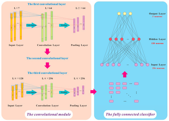
Figure 13.
The model architecture of this study.
Table 4.
Details of the model architecture.
The classifier section consists of one Dropout layer (a dropout rate of 0.5), a fully connected layer with 128 neurons, and a ReLU activation function (Equation (2)), which further integrates the extracted convolutional features and mitigates overfitting risks [32]. The final output layer is a fully connected layer corresponding to three target classes: non-reservoir, water layer, and oil-bearing layer. Different window lengths were tested to evaluate their effects on the receptive field and predictive stability of the CNN (Table 5).
Table 5.
Sensitivity analysis of depth-wise input segment length.
The experimental results indicate that overly short input segments fail to capture sufficient vertical context, whereas excessively long segments may introduce irrelevant stratigraphic information across multiple depositional units. Based on this analysis, a moderate window length of L = 16 depth samples was selected, which corresponds to approximately 2 m in vertical depth given the sampling interval of 0.125 m. This window length achieves the optimal balance between contextual information and geological consistency, and is well aligned with the typical thickness of individual tight sandstone layers in the Chang 8 Formation. This window slides with a stride of L/2, resulting in a 50% overlap between adjacent segments. The reservoir label of each segment is assigned according to the reservoir type at the central depth sample, ensuring geological consistency between the input features and the target label. Furthermore, Global Average Pooling is employed in the final convolutional module to aggregate depth-wise features into a fixed-length representation, thereby enabling the network to accommodate variable well lengths without padding or truncation.
3.4.3. Loss Function
In traditional classification tasks, model optimization is achieved by minimizing the cross-entropy loss function (), enhancing the accuracy of model predictions [33]. The main expression is depicted as Equation (4).
where the total number of samples in the training set and the number of categories in the oil and gas reservoir formations are represented by and , respectively. The actual value for a category and the value predicted by the model for that category are denoted as and , respectively.
The traditional cross-entropy loss treats all samples equally. However, in classification tasks where differences in class difficulty and class imbalance exist, the model tends to be dominated by easily classified and majority classes. Given that the dataset in this study shows a clear class imbalance (with 5930 non-reservoir layer samples, 1031 oil-bearing layer samples, and only 145 water layer samples), and considering the importance and economic value of accurately identifying oil-bearing layers in hydrocarbon exploration, Focal Loss was introduced as the loss function to ensure that the model is better able to detect potential oil-bearing layers [34].
Focal Loss addresses this issue through its core design concept—adaptive balancing between easy and hard samples. It dynamically adjusts the model’s focus to “hard samples” (those difficult to classify correctly) and “easy samples” (those easy to classify correctly), thereby mitigating the impact of class imbalance and improving model performance. By introducing a modulating factor (γ) and class weight (), Focal Loss reduces the loss contribution of easily classified samples (non-reservoir), compelling the model to pay greater attention to hard-to-classify samples (oil-bearing layer). Mathematically, this can be expressed as Equation (5).
where
- denotes the predicted probability for the true class of a sample. For a given true class label y, if y = 1, then ; if y = 0, then .
- is the focusing parameter (where γ ≥ 0), which controls the weighting between easy and hard samples. A higher value of γ downweights the loss contribution from easy examples more strongly. In this study, we set = 4 (validated through ablation experiments with = 0/2/4/6; when = 4, the recall rate of oil-bearing layers is the highest while preventing the model from over-focusing on hard-to-classify samples).
- is the class weighting factor that dynamically adjusts the weight based on the true class of the sample. This helps mitigate class imbalance by assigning higher importance to underrepresented classes during training. In this study, was set empirically as [1, 20, 20] for [non-reservoir, water layer, oil-bearing layer], respectively, to counterbalance the class distribution (these values were selected based on preliminary grid search and prior studies on imbalanced geophysical data classification).
By adjusting the two hyperparameters, and , the attention level of focal loss to samples of different categories and difficulty levels can be controlled. In this way, the model focuses more on learning challenging-to-classify samples, improving training effectiveness in the presence of class imbalance. This enhances the model’s robustness and generalization ability, preventing it from being dominated by the loss of many easily classifiable samples. This mechanism makes focal loss more effective than the traditional cross-entropy loss function when dealing with class imbalance and challenging-to-classify samples.
3.4.4. Optimization Algorithm
For the optimizer, this study employs the Adam optimization algorithm [35]. Adam combines the advantages of Momentum and AdaGrad, adaptively adjusting the learning rate of different parameters based on the first and second moments of the gradients. This property enables faster convergence and greater stability during the training of deep learning models, making it particularly suitable for scenarios with limited data and imbalanced class distributions, as in this study.
The specific parameter settings are as follows: the initial learning rate is 0.001, and the weight decay coefficient is 1 × 10⁻⁴, which penalizes large weights to mitigate overfitting and enhance the model’s generalization capability. Additionally, a StepLR learning rate scheduler is introduced, reducing the learning rate to one-tenth of its previous value every 30 epochs. This mechanism allows the model to maintain a relatively high learning rate in the early stages for rapid convergence and a lower learning rate in later stages for fine parameter adjustment, thereby improving performance on both the validation and test sets. Finally, the model is trained for 100 epochs with a batch size of 32, combining the Adam optimizer with the StepLR scheduler to achieve stable convergence under limited sample conditions.
4. Results
4.1. Model Performance Evaluation Methods
The confusion matrix is a critical tool for evaluating the performance of classification models, particularly in binary and multiclass tasks. It presents the alignment between the predicted and actual outcomes in a matrix format, providing a comprehensive representation of the model’s classification performance and its behavior across different categories. Typically, the confusion matrix is an n × n matrix, where n denotes the number of classes. In this study, there are three categories: The oil-bearing layer, the water layer, and the non-reservoir.
For multiclass classification problems, each row of the confusion matrix represents the distribution of samples for a specific actual class, whereas each column corresponds to the number of samples predicted as a particular class by the model. The diagonal elements indicate the number of correctly predicted samples, whereas the off-diagonal elements reflect the degree of misclassification between different categories. The core metrics include the following.
True positive (TP): Refers to the number of samples correctly classified as belonging to a specific class. For a given class, this corresponds to the diagonal element of the confusion matrix, which represents the actual samples of that class that were correctly identified.
False positive (FP): Refers to the number of samples from other classes that were incorrectly predicted as belonging to a specific class. For a given class i, FP is the sum of the off-diagonal elements in column i of the matrix.
False negative (FN): Refers to the number of samples from a specific class that were incorrectly predicted as belonging to other classes. For a given class i, FN is the sum of the off-diagonal elements in row i of the matrix.
Based on the core metrics mentioned above, several performance indicators can be calculated to evaluate the classification model:
Accuracy: Measures the proportion of correctly predicted samples to the total number of samples in a classification model. The main expression is depicted as Equation (6).
This reflects the overall prediction accuracy of the model across all classes.
Recall: Measures the proportion of actual samples of a specific class that are correctly predicted by the model. The main expression is depicted as Equation (7).
This reflects the model’s ability to identify positive samples for a given class.
Precision: Measures the proportion of samples predicted as a specific class that actually belong to that class. The main expression is depicted as Equation (8).
This indicates the accuracy of the model’s positive predictions for a given class.
F1 Score: The harmonic mean of Precision and Recall, providing a balanced measure that considers both false positives and false negatives. It is particularly useful when the class distribution is imbalanced. The main expression is depicted as Equation (9).
The F1 Score offers a comprehensive reflection of the model’s performance for a given class.
In this study, Accuracy, Recall, Precision, and F1 Score were computed based on the confusion matrix. Importantly, in this regional dataset, the non-reservoir accounts for 83%, the water layer accounts for 2%, and the oil-bearing layer accounts for 15%. Thus, the data distribution is imbalanced. In tasks with extremely imbalanced data, such as this study, besides focusing on Accuracy, high Recall is more meaningful than high Precision. This is because, in the present study, the class with fewer samples (the oil-bearing layer) has a higher economic value, and identifying more instances of the minority class is crucial. Consequently, missing the oil-bearing layer often results in significant losses compared with misclassifying other reservoir types as the oil-bearing layer. Therefore, in this study, Accuracy and Recall are adopted as the primary evaluation metrics.
4.2. Experimental Results and Performance Evaluation
4.2.1. Identification Performance of Different Models
To fully evaluate the identification performance of the proposed model, we compared it with several other deep learning models and machine learning models, including CNN-LSTM, DeeperWiderCNN, and random forest (RF). The confusion matrices of different models on the validation set after training are shown in Figure 14.
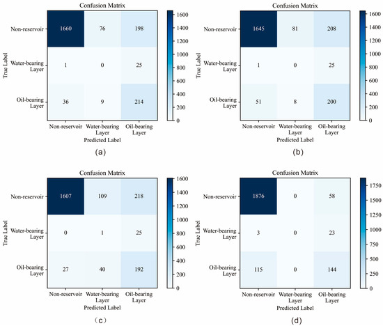
Figure 14.
Model validation confusion matrices: (a) convolutional neural network (CNN); (b) convolutional neural network-long short-term memory (CNN-LSTM); (c) deeper and wider convolutional neural network (DeeperWiderCNN); (d) random forest (RF).
Based on the confusion matrix, the remaining evaluation metrics are calculated for all the models (Table 6, Table 7 and Table 8).
Table 6.
Accuracy of different models.
Table 7.
Recall of different models.
Table 8.
F1 Score of different models.
The experimental results indicate that, compared with other deep learning models and machine learning models, the CNN model designed in this study delivered the best overall performance in reservoir identification. It attained a high Accuracy of 84% on the validation set and achieved the highest Recall for oil-bearing layers (83%). Although the machine learning model (RF) exhibited slightly higher Accuracy, it had the lowest Recall for oil-bearing layers, with nearly 50% of oil-bearing samples being missed. The other two deep learning models also exhibited relatively low Recall.
To further comprehensively evaluate the performance of each model under class imbalance conditions, we plotted Receiver Operating Characteristic (ROC) curves for analysis. Considering that oil-bearing layer samples are the key minority class, Figure 15 shows the ROC curves of each model for the oil-bearing layer category, while Figure 16 presents the multiclass micro-average ROC curves.
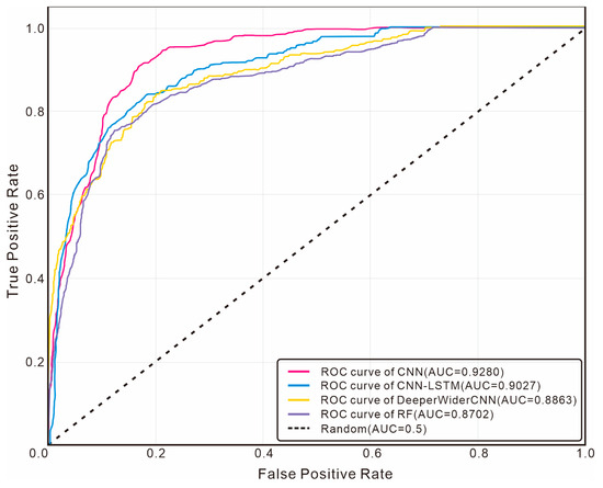
Figure 15.
Comparison of ROC curves of different models for the oil-bearing layer category.
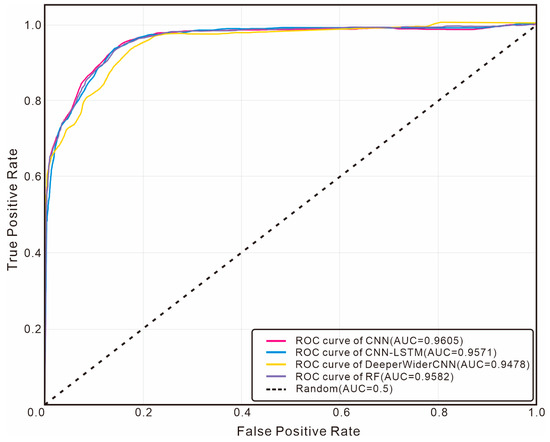
Figure 16.
Comparison of micro-average ROC curves among different models.
As can be seen from the ROC curves for the oil-bearing layer category, the AUC value of the CNN model proposed in this study reaches 0.9280, which is significantly higher than that of CNN-LSTM (0.9027), DeeperWiderCNN (0.8863), and Random Forest (0.8702). This result indicates that the CNN model has stronger discriminative ability in distinguishing oil-bearing layers from non-oil-bearing layers. Its curve is closer to the upper left corner, demonstrating that it can achieve a higher true positive rate at the same false positive rate. From the analysis of the micro-average ROC curves, the micro-average AUC of the CNN model is 0.9605, which is also superior to other comparative models.
4.2.2. Performance of Models Using Different Loss Functions
To evaluate the effectiveness of Focal Loss in enhancing the model’s identification performance, two additional loss functions were employed for comparative analysis. The confusion matrices for the deep learning model with different loss functions on the validation set are shown in Figure 17.
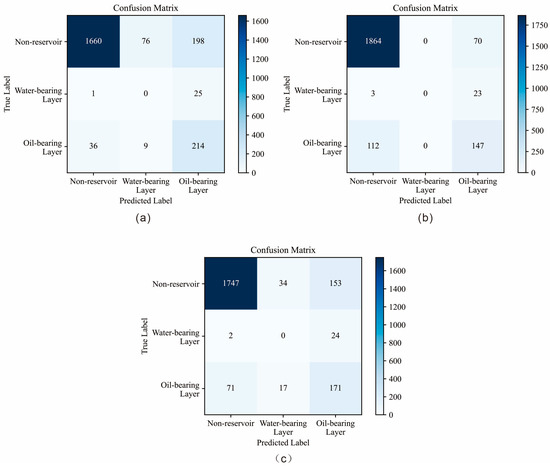
Figure 17.
Model validation confusion matrices: (a) Focal Loss function; (b) Traditional cross-entropy loss function; (c) Class-weighted cross-entropy loss function.
Based on the confusion matrices, the remaining evaluation metrics for all the models were calculated (Table 9, Table 10 and Table 11).
Table 9.
Accuracy of models with different loss functions.
Table 10.
Recall of models with different loss functions.
Table 11.
F1 Score of models with different loss functions.
The experimental results indicate that, compared with CNN models using other loss functions, the CNN model using Focal Loss achieved the best overall performance in reservoir identification. Although its Accuracy on the validation set (84%) was slightly lower than that of the other two loss functions, the difference was negligible. More importantly, its Recall for oil-bearing layers was significantly higher, demonstrating a superior ability to capture potential oil-bearing layer samples to the greatest extent.
To further explore the impact of loss functions on model performance under class imbalance conditions, we plotted additional ROC curves corresponding to different loss functions. Figure 18 shows the ROC curves of each loss function for the oil-bearing layer category, while Figure 19 presents the micro-average ROC curves.
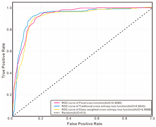
Figure 18.
Comparison of ROC curves of loss functions for the oil-bearing layer category.
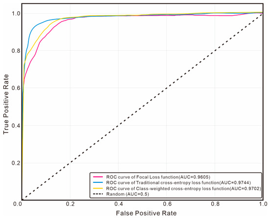
Figure 19.
Comparison of Micro-average ROC Curves Among Different Loss Functions.
In terms of oil-bearing layer identification, the AUC value of Focal Loss is 0.9280, which is slightly higher than that of traditional cross-entropy loss (0.9243) and significantly higher than that of class-weighted cross-entropy loss (0.9089). This indicates that through its dynamic modulation mechanism, Focal Loss effectively enhances the model’s attention to the key minority class, enabling it to perform better in the oil-bearing layer identification task. In the micro-average ROC curve, traditional cross-entropy loss achieves the highest AUC value (0.9744), which is higher than that of Focal Loss (0.9605). This reveals that traditional cross-entropy tends to optimize the overall accuracy, while Focal Loss focuses on improving the identification ability of the minority class.
4.3. Sensitivity Analysis
Sensitivity analysis plays an important role in quantifying the influence of each input parameter on the model outputs, helping to identify the most effective features and guiding model interpretation and optimization. For instance, Jolfaei and Lakirouhani [36] employed the cosine amplitude method (CAM) in conjunction with a neural network to conduct sensitivity analysis on the parameters affecting borehole breakout dimensions. In this study, we adopted the concept of sensitivity analysis and implemented it using mutual information to measure the dependency between each well-logging parameter and the target variable (reservoir type). A higher mutual information value indicates that a feature contains more target-related information and thus has a stronger impact on the model. To identify key well-logging parameters, we calculated mutual information scores between each feature and the target, and the calculation results are shown in Figure 20.
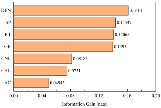
Figure 20.
Mutual information ranking for well-logging parameters.
5. Discussion
5.1. Comparison with Other Models
This study utilizes real well-logging data from the Jiyuan Oilfield in the Ordos Basin to develop an intelligent identification model aimed at assisting in the interpretation of well-logging information. By conducting comparative experiments among the proposed CNN model, more complex deep learning models (CNN-LSTM and DeeperWiderCNN), and a traditional and widely used machine learning model (RF), the results demonstrate that the CNN model achieves the highest recall rate for oil-bearing layers while maintaining high accuracy across all categories. This indicates that the model effectively balances the classification boundaries among different classes and minimizes the omission of oil-bearing layers—a category with high economic value in practical exploration scenarios. ROC analysis also reveals that the CNN model not only exhibits stable performance in terms of overall accuracy but also demonstrates greater robustness in identifying the key minority class (oil-bearing layers) under class imbalance conditions.
These findings verify that the proposed model can more comprehensively capture the intrinsic relationships between tight, heterogeneous reservoirs and various well-logging parameters, accurately and intelligently extract key well-logging features, and thus achieve the research objectives.
5.2. Impact of Loss Function Design
When different loss functions were applied to the proposed model, the results revealed that the traditional cross-entropy loss function could not overcome the challenges posed by sample imbalance—specifically, it failed to effectively focus on and capture the characteristics of minority-class samples. Although the model achieved relatively high overall accuracy (primarily due to the correct classification of majority classes), it missed a substantial portion of oil-bearing layer samples, which are of high economic importance in practical exploration scenarios. By introducing the class-weighted cross-entropy loss function, this issue was partially alleviated, leading to an improvement in the recall rate for oil-bearing layers. Finally, by employing the Focal Loss, the model achieved the optimal performance: it attained the highest recall rate for minority-class samples while maintaining high overall accuracy, effectively balancing both objectives. ROC analysis indicates that although the model using Focal Loss has a slightly lower micro-average AUC, it exhibits stronger ability in identifying the key target class (oil-bearing layers), which is more in line with the practical needs in hydrocarbon exploration.
These results demonstrate that optimizing the loss function can effectively mitigate the issue of class imbalance in reservoir identification tasks and significantly enhance the identification performance for oil-bearing layers.
5.3. Dependence of Reservoir Identification on Key Well-Logging Parameters
Mutual information reveals the importance ranking of well-logging parameters in reservoir identification within low-permeability reservoirs: DEN, SP, RT, and GR are core parameters, whereas CNL, CAL, and AC serve as auxiliary parameters. This result is highly consistent with petroleum geological theory, revealing the dominant controlling factors in reservoir identification within the study area.
DEN emerges as the most significant feature, directly reflecting the physical properties of rocks and effectively distinguishing lithologies while assessing the degree of pore development. SP and GR, as key indicators of permeability and lithology, respectively, jointly determine the presence or absence of effective reservoirs. Although RT plays a crucial role in fluid identification, its contribution to reservoir identification is slightly lower than that of DEN and SP, reflecting the logical sequence of “identifying reservoirs before distinguishing fluids.” CNL and AC contribute to porosity estimation, whereas CAL primarily provides information on borehole quality; thus, these three parameters show relatively limited influence.
This feature-importance ranking not only verifies the geological interpretability of the machine learning results but also provides a quantitative basis for optimizing feature selection in reservoir identification models. It demonstrates that a feature combination based on DEN–SP–RT–GR can effectively capture the core geological information for reservoir identification in the study area, offering valuable references for well-logging interpretation under similar geological settings.
5.4. Model Application
Based on the reservoir identification model developed in this study, blind-well testing was conducted on well Huang488 within the study area.
The blind-well test results of Well Huang488 (Figure 21, Table 12) show that the overall accuracy of the model reaches 85%, and the recall rate of oil-bearing layers is 96%. The blind-well test results fully validate the identification performance of the CNN model enhanced with Focal Loss, providing a new auxiliary approach for the secondary interpretation of well-logging data from old wells and for reservoir identification within the study area. For field use, the model can be encapsulated into a software module or API, allowing geologists to upload log data and receive instant identification results, thereby significantly improving interpretation efficiency in tight sandstone exploration.
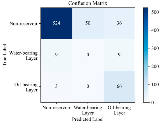
Figure 21.
The confusion matrix for blind-well data identification.
Table 12.
The results of blind-well data identification.
However, all water layer samples were misclassified, which is directly related to the extremely small number of water layer samples in the training dataset. In the future, we plan to expand the dataset in both size and diversity by exploring new data acquisition methods and channels. These efforts will help to address the current limitations and enhance the comprehensiveness and robustness of the research.
5.5. Limitations and Future Work
Although the model proposed in this study achieves high accuracy in oil-bearing layer identification, it still has certain limitations, mainly reflected in the following two aspects:
First, the model exhibits a high misclassification rate in water layer identification, with the main reasons including:
- The proportion of water layer samples in the dataset is extremely low (only about 2%), leading to certain limitations in the model’s ability to learn water layer characteristics.
- The well-logging response characteristics of water layers overlap with those of other lithological types in some aspects, which further increases the difficulty of classification.
Second, the method in this study is constructed and validated under the premise that well-logging curves are complete and available and does not explicitly consider the problem of missing well-logging curves that may occur in actual production processes. In real hydrocarbon exploration scenarios, due to instrument failure, complex well conditions, or restricted construction conditions, some well-logging parameters may be missing or incomplete, which, to a certain extent, affects the applicability and prediction stability of the model.
To address the above limitations, future research will further improve the model’s performance and engineering applicability from the following aspects:
- Introduce Synthetic Minority Oversampling Technique (SMOTE) to expand the scale of water layer samples and alleviate the class imbalance problem.
- Adopt a cost-sensitive learning strategy and assign higher penalty weights to water layer misclassification to improve the model’s ability to identify water layers.
- Bidirectionally optimize model performance through transfer learning technology. On the one hand, use water layer data from adjacent blocks to pre-train the model to enhance its water layer identification ability; on the other hand, pre-train based on large-scale complete well-logging data and combine it with small-sample fine-tuning of data with missing curves to improve the model’s adaptability to missing well-logging curves.
- Further explore robust modeling strategies for scenarios with missing well-logging curves, such as combining well-logging curve imputation methods or introducing missing-aware network structures, to enhance the model’s application potential under actual complex working conditions.
6. Conclusions
This study developed an intelligent reservoir identification framework based on convolutional neural networks and applied it to well-logging data from the Chang 8 Formation in the Jiyuan area of the Ordos Basin. By integrating deep learning with geological constraints, the proposed approach provides a practical and reliable solution for automated reservoir identification in tight sandstone reservoirs.
First, a well-based data partitioning strategy was adopted to evaluate model performance at the well scale rather than at the sample scale. This design effectively avoids the overoptimistic bias commonly introduced by random sample splitting and allows a more realistic assessment of the model’s generalization capability to unseen wells, which is critical for field-scale applications.
Second, the introduction of Focal Loss significantly enhanced the model’s ability to handle severe class imbalance inherent in reservoir identification tasks. By adaptively focusing on hard-to-classify and high-value minority-class samples, the proposed CNN model achieved a substantially improved identification capability for oil-bearing layers, demonstrating the effectiveness of loss function design in geophysical deep learning applications.
Third, the mutual information–based feature-importance analysis provided clear physical interpretability of the model results. The identification of DEN, SP, RT, and GR as key controlling parameters is consistent with established petroleum geological theory, confirming that the proposed model not only achieves high predictive performance but also preserves meaningful geological insights.
Overall, this study demonstrates that combining a rigorous evaluation framework, imbalance-aware optimization, and interpretable feature analysis can significantly improve the reliability and applicability of deep learning methods for reservoir identification. Future work will focus on expanding the dataset, particularly for underrepresented reservoir types, and exploring advanced imbalance-handling strategies, such as data augmentation and transfer learning, to further enhance model robustness and generalization performance.
Author Contributions
Conceptualization, W.L.; methodology, W.L. and L.L.; software, W.L. and L.L.; investigation, W.L.; resources, D.L.; data curation, D.L.; writing—original draft preparation, W.L.; writing—review and editing, Z.Z.; supervision, Z.H.; validation, Z.H.; project administration, D.L.; funding acquisition, Z.Z. All authors have read and agreed to the published version of the manuscript.
Funding
This study was supported by the Shaanxi Youth Science and Technology Star Project (Grant No. 2021KJXX-87) and Shaanxi Public Welfare Geological Survey Project (Grant Nos. 20180301, 201918, and 202103).
Data Availability Statement
The data presented in this study are available on request from the corresponding author due to the fact that the oilfield-provided well-logging data are confidential in nature and contain economic value.
Acknowledgments
The authors would like to express their most sincere gratitude to the field workers in the Jiyuan Oilfield. The authors also thank the anonymous reviewers for their valuable comments and suggestions and the scholars for their guidance on the paper.
Conflicts of Interest
Author Dongtao Li was employed by the The Fifth Oil Production Plant of PetroChina Changqing Oilfield Company. The remaining author declares that the research was conducted in the absence of any commercial or financial relationships that could be construed as a potential conflict of interest.
References
- Peng, Z.; Yang, H.; Pan, H.; Ji, Y. Identification of Low Resistivity Oil and Gas Reservoirs with Multiple Linear Regression Model. In Proceedings of the 2016 12th International Conference on Natural Computation, Fuzzy Systems and Knowledge Discovery (ICNC-FSKD), Changsha, China, 13–15 August 2016; IEEE: Piscataway, NJ, USA, 2016; pp. 529–533. [Google Scholar] [CrossRef]
- Fang, S.; Lin, Z.; Zhang, Z.; Zhang, C.; Pan, H.; Du, T. Gas Hydrate Saturation Estimates in the Muli Permafrost Area Considering Bayesian Discriminant Functions. J. Pet. Sci. Eng. 2020, 195, 107872. [Google Scholar] [CrossRef]
- Li, X.; Shi, Y.J.; Wang, L.; Hu, S. Logging Identification and Evaluation Technique of Tight Sandstone Gas Reservoirs: Taking Sulige Gas Field as an Example. Nat. Gas Geosci. 2013, 24, 62–68. Available online: http://www.nggs.ac.cn/CN/10.11764/j.issn.1672-1926.2013.01.62 (accessed on 29 December 2025).
- Luo, S.; Hu, G.; Li, L.; Wang, J.; Li, X. Genetic Analysis and Well-Log Evaluation of the Productivity Simulation for Unconventional Gas Reservoirs of Tight Sanstone: A Case from B Gas Reservoirs in A Sag. Prog. Geophys. 2015, 30, 2714–2722. [Google Scholar] [CrossRef]
- Wang, D. Study on the Rock Physics Model of Gas Reservoirs in Tight Sandstone. Chin. J. Geophys. 2016, 59, 4603–4622. [Google Scholar] [CrossRef]
- Das, B.; Chatterjee, R. Well Log Data Analysis for Lithology and Fluid Identification in Krishna-Godavari Basin, India. Arab. J. Geosci. 2018, 11, 231. [Google Scholar] [CrossRef]
- Yang, W.; Sun, J.; Du, Q.; Zhang, Y.; Luo, X. Fluid Property Identification Method for Low Permeability Reservoirs Based on SMOTE Sampling and Integrated Learning. Well Logging Technol. 2025, 49, 1–9. [Google Scholar] [CrossRef]
- Fang, S.; Zhang, Z.; Chen, W.; Pan, H.; Peng, J. 3D Crosswell Electromagnetic Inversion Based on Radial Basis Function Neural Network. Acta Geophys. 2020, 68, 711–721. [Google Scholar] [CrossRef]
- Fang, S.; Zhang, Z.; Wang, Z.; Pan, H.; Du, T. Principal Slip Zone Determination in the Wenchuan Earthquake Fault Scientific Drilling Project-Hole 1: Considering the Bayesian Discriminant Function. Acta Geophys. 2020, 68, 1595–1607. [Google Scholar] [CrossRef]
- Tan, M.; Bai, Y.; Zhang, H.; Li, G.; Wei, X.; Wang, A. Fluid typing in tight sandstone from wireline logs using classification committee machine. Fuel 2020, 271, 117601. [Google Scholar] [CrossRef]
- Yan, X.; Cao, H.; Yao, F.; Ba, J. Bayesian lithofacies discrimination and pore fluid detection in tight sandstone reservoir. Oil Geophys. Prospect. 2012, 47, 945–950. [Google Scholar] [CrossRef]
- Cheng, C.; Li, P.; Chen, Y.; Ye, Y.; Gao, Y.; Zhang, L. Research Progress of Reservoir Logging Evaluation Based on Machine Learning. Prog. Geophys. 2022, 37, 164–177. [Google Scholar] [CrossRef]
- Zhang, J.; He, Y.; Zhang, Y.; Li, W.; Zhang, J. Well-Logging-Based Lithology Classification Using Machine Learning Methods for High-Quality Reservoir Identification: A Case Study of Baikouquan Formation in Mahu Area of Junggar Basin, NW China. Energies 2022, 15, 3675. [Google Scholar] [CrossRef]
- Zhou, X.; Li, Y.; Song, X.; Jin, L.; Wang, X. Thin Reservoir Identification Based on Logging Interpretation by Using the Support Vector Machine Method. Energies 2023, 16, 1638. [Google Scholar] [CrossRef]
- Han, Y. Intelligent Fluid Identification Based on the AdaBoost Machine Learning Algorithm for Reservoirs in Daniudi Gas Field. Pet. Drill. Technol. 2022, 50, 112–118. [Google Scholar] [CrossRef]
- Liu, M.; Jervis, M.; Li, W.; Nivlet, P. Seismic Facies Classification Using Supervised Convolutional Neural Networks and Semisupervised Generative Adversarial Networks. Geophysics 2020, 85, 047–058. [Google Scholar] [CrossRef]
- Qi, M.; Han, C.; Ma, C.; Liu, G.; He, X.; Li, G.; Yang, Y.; Sun, R.; Cheng, X. Identification of Diagenetic Facies Logging of Tight Oil Reservoirs Based on Deep Learning—A Case Study in the Permian Lucaogou Formation of the Jimsar Sag, Junggar Basin. Minerals 2022, 12, 913. [Google Scholar] [CrossRef]
- Luo, G.; Xiao, L.; Shi, Y.; Shao, R. Machine Learning for Reservoir Fluid Identification with Logs. Pet. Sci. Bull. 2022, 7, 24–33. [Google Scholar] [CrossRef]
- Shi, Y.; Liao, J.; Gan, L.; Tang, R. Lithofacies Prediction from Well Log Data Based on Deep Learning: A Case Study from Southern Sichuan, China. Appl. Sci. 2024, 14, 8195. [Google Scholar] [CrossRef]
- Farahnakian, F.; Sheikh, J.; Zelioli, L.; Nidhi, D.; Seppä, I.; Ilo, R.; Nevalainen, P.; Heikkonen, J. Addressing Imbalanced Data for Machine Learning Based Mineral Prospectivity Mapping. Ore Geol. Rev. 2024, 174, 106270. [Google Scholar] [CrossRef]
- Banar, S.; Mohammadi, R. SeismoNet: A Proximal Policy Optimization-Based Earthquake Early Warning System Using Dilated Convolution Layers and Online Data Augmentation. Expert Syst. Appl. 2024, 253, 124337. [Google Scholar] [CrossRef]
- Kazemi, A.; Esmaeili, M. Mitigating Data Imbalance in Semantic Segmentation Using Sequential Unconditional and Conditional Diffusion Models: A Case Study in Digital Rock Physics. Neural Comput. Appl. 2025, 37, 26079–26098. [Google Scholar] [CrossRef]
- Li, P.; Meng, J.B.; Li, J.; Chen, Q.J. Enhanced Lithofacies Classification of Tight Sandstone Reservoirs Using a Hybrid CNN-GRU Model with BSMOTE and Heat Kernel Imputation. Appl. Geophys. 2025, 22, 1–17. [Google Scholar] [CrossRef]
- Zhang, Z.; Li, Y.; Wang, G.; Carranza, E.J.M.; Yang, S.; Sha, D.; Fan, J.; Zhang, X.; Dong, Y. Supervised Mineral Prospectivity Mapping via Class-Balanced Focal Loss Function on Imbalanced Geoscience Datasets. Math. Geosci. 2023, 55, 989–1010. [Google Scholar] [CrossRef]
- He, T.; Zhou, Y.; Li, Y.; Xie, H.; Shang, Y.; Chen, T.; Zhang, Z. Research on the Microscopic Pore-Throat Structure and Reservoir Quality of Tight Sandstone Using Fractal Dimensions. Sci. Rep. 2024, 14, 22825. [Google Scholar] [CrossRef]
- Liu, H.; Li, X.; Wan, Y. Palaeogeographic and sedimentological characteristics of the Triassic Chang 8, Ordos Basin, China. Acta Sedimentol. Sin. 2011, 29, 1086–1095. [Google Scholar] [CrossRef]
- Chu, M.; Guo, Z.; Bai, C. Sedimentation and evolution features in Chang 8 reservoir of Yanchang Formation in Ordos Basin. J. Oil Gas Technol. 2012, 34, 13–18. [Google Scholar]
- LeCun, Y.; Bengio, Y.; Hinton, G. Deep Learning. Nature 2015, 521, 436–444. [Google Scholar] [CrossRef]
- Kiranyaz, S.; Avci, O.; Abdeljaber, O.; Ince, T.; Inman, D.J. 1D Convolutional Neural Networks and Applications: A Survey. Mech. Syst. Signal Process. 2021, 151, 107398. [Google Scholar] [CrossRef]
- Nair, V.; Hinton, G.E. Rectified Linear Units Improve Restricted Boltzmann Machines. In Proceedings of the 27th International Conference on Machine Learning (ICML-10), Haifa, Israel, 21–24 June 2010; pp. 807–814. [Google Scholar]
- Ioffe, S.; Szegedy, C. Batch Normalization: Accelerating Deep Network Training by Reducing Internal Covariate Shift. In Proceedings of the 32nd International Conference on Machine Learning: ICML 2015, Lile, France, 6–11 July 2015. [Google Scholar] [CrossRef]
- Srivastava, N.; Hinton, G.; Krizhevsky, A.; Sutskever, I.; Salakhutdinov, R. Dropout: A Simple Way to Prevent Neural Networks from Overfitting. J. Mach. Learn. Res. 2014, 15, 1929–1958. Available online: https://jmlr.org/papers/v15/srivastava14a.html (accessed on 29 December 2025).
- Andreieva, V.; Shvai, N. Generalization of Cross-Entropy Loss Function for Image Classification. Mohyla Math. J. 2021, 3, 3–10. [Google Scholar] [CrossRef]
- Lin, T.-Y.; Goyal, P.; Girshick, R.; He, K.; Dollar, P. Focal Loss for Dense Object Detection. IEEE Trans. Pattern Anal. Mach. Intell. 2020, 42, 318–327. [Google Scholar] [CrossRef] [PubMed]
- Kingma, D.; Ba, J. Adam: A Method for Stochastic Optimization. arXiv 2014. [Google Scholar] [CrossRef]
- Jolfaei, S.; Lakirouhani, A. Sensitivity Analysis of Effective Parameters in Borehole Failure, Using Neural Network. Adv. Civil Eng. 2022, 2022, 4958004. [Google Scholar] [CrossRef]


Disclaimer/Publisher’s Note: The statements, opinions and data contained in all publications are solely those of the individual author(s) and contributor(s) and not of MDPI and/or the editor(s). MDPI and/or the editor(s) disclaim responsibility for any injury to people or property resulting from any ideas, methods, instructions or products referred to in the content. |
© 2026 by the authors. Licensee MDPI, Basel, Switzerland. This article is an open access article distributed under the terms and conditions of the Creative Commons Attribution (CC BY) license.