Multi-Objective Path Planning for Warehouse Inspection of Mobile Robots Considering Power Limitations and Multiple Charging Points

Abstract

In large-scale warehouses, mobile robots often face energy shortages during inspection tasks, necessitating multiple charging points. Considering battery limits and multiple charging points makes path planning challenging. This paper presents a two-level solution: (i) local path planning via improved B-RRT* (adaptive Gaussian sampling + dynamic goal bias) to build a path-cost matrix, and (ii) global inspection and charging scheduling under multi-charging-point constraints. We evaluate planning time, total path length (as an energy proxy), and the number of sampling points. Experimental results demonstrate that the improved B-RRT* algorithm achieves an average reduction of 10–15% in path length, 20–30% in computation time, and 15–40% in the number of sampling points compared to the initial B-RRT* and RRT* algorithms across various warehouse environments. For global planning with up to 60 inspection targets and 3–5 charging points, a feasible charging schedule is obtained within 150–360 s on a standard desktop (Ryzen 7 5800H, 16 GB RAM), demonstrating strong practicality and scalability.

1. Introduction

With the rapid development of robotics, mobile robots have gradually transitioned from laboratory research to practical applications in various fields of society. Warehouse inspection, maintenance, and testing emerge as critical applications in industrial automation. However, there are bottlenecks in the battery technologies, which cannot support mobile robots operating for extended periods without recharging. It is often necessary to charge them at designated charging points during operation. Ensuring stable and continuous operation through automated and efficient charging scheduling during inspections has become a key research focus. For example, Pei et al. [1] addressed the charging scheduling problem of automatic carrier robots in flexible automated logistics warehouse operation. They constructed a scheduling model with the optimization objective of minimizing weighted charging completion time in order to maximize the utilization rate of robots in warehouse operation. Ravankar et al. [2], aiming to solve the problem of multi-robot charging scheduling in warehouse inspection, designed an intelligent path-planning process for charging scheduling by systematically considering the remaining power, task priority, and location of the robot. Aiming at the problem of automatic charging path planning for cleaning robots in complex industrial environments, Hao et al. [3] constructed two models, with designated charging locations and multiple charging locations, and used the Dijkstra algorithm and fruit fly optimization algorithm to adjust path nodes and shorten path length, respectively. Similar to the charging scheduling problem of mobile robots, there are also many studies on electric vehicle charging scheduling. Among them, Li Zhufeng [4] established a distribution path-planning model for electric logistics vehicles considering different power replenishment methods in the process of electric logistics vehicle distribution, and used the artificial fish swarm algorithm to solve the model. Yuan Jiaxin [5] et al. constructed a model aiming to minimize the total operating cost for the electric bus charging scheduling problem, and used CPLEX to solve it. Mahnoosh [6] et al. constructed a charging decision model for a single EV, considering the influencing factors of EV charging location, related charging amount, and location-based electricity price, and used virtual connections with negative energy demand to extend the original traffic diagram to represent the charging options available to users.

Warehouse inspection is fundamentally characterized as a multi-objective point path-planning problem. This type of planning necessitates that the initial point traverses all designated target points before returning to the terminal point. The problem can be segmented into two components: the local path-planning problem, which involves the navigation between the starting point, the ending point, and any two target points, and the global path-planning problem, which pertains to the sequence of multi-objective point inspections. Currently, path planning between two points predominantly employs algorithms such as A* [7], RRT [8], and Dijkstra [9]. Notably, the sampling-based RRT algorithm demonstrates superior adaptability to dynamic and complex environments compared to the A* and Dijkstra algorithms, making it particularly suitable for warehouse inspection path planning. However, a limitation of the RRT algorithm is that the search tree expands in a blind and redundant manner, resulting in suboptimal path quality. To address these challenges, Zhang Tenglong et al. [10] introduced a dynamic bidirectional asymptotic optimal fast random expansion tree algorithm with a fixed number of nodes, which enhances path search speed through a bidirectional greedy search approach while reducing computational demands by constraining the number of nodes in the search tree, thereby facilitating rapid path discovery. Similarly, Meng Wenlong et al. [11] proposed an improved RRT-Connect algorithm that integrates adaptive circular sampling with a dynamic step size to minimize the generation of redundant sampling points, thereby enhancing the efficiency of local path planning. Fu Yunlai et al. [12] developed a path-planning algorithm based on an improved P-RRT*, which incorporated a target bias strategy and restricted the expansion angle of the random tree during the sampling process to boost path search efficiency. Zhao et al. [13] introduced a dynamic RRT algorithm that estimates the path length from the starting node to the target node, utilizing this length heuristically as the principal axis diameter of the informed subset, thereby centralizing new node sampling to optimize the estimated path. Furthermore, Sivasankar et al. [14] proposed a hybrid sampling RRT* algorithm that generates samples in both uniform and non-uniform manners, ultimately enhancing path search efficiency. Lastly, Wu et al. [15] presented an improved Fast-RRT algorithm, which augments the path search efficiency of the RRT* algorithm by incorporating a fast sampling strategy and a random turning strategy expansion approach, effectively addressing the issue of inadequate search performance in narrow channels. The multi-objective path-planning problem is essentially the same as the traveling salesman problem. As an NP-hard problem, the TSP takes a lot of time to accurately obtain a solution. Therefore, at present, heuristic algorithms are usually used to obtain a better solution within the allowable tolerance. Wang et al. [16] proposed an improved ant colony optimization algorithm to solve the TSP, and used hybrid symbiotic organism search to adaptively optimize the parameters of the ant colony algorithm. Gharehchopogh [17] et al. proposed a Harris Hawk Optimization (HHO) method for an improved scheme of random key coding generation. In addition to the main strategy of the HHO algorithm in the exploration phase, this method also adopts the mutation mechanism in the development phase. Huang et al. [18] presented an enhanced Gaussian-biased bidirectional rapidly exploring random tree. They constructed a multi-level sampling weight function based on obstacle distribution, by restricting random tree sampling in invalid regions and focusing sampling points on high-probability path areas, thus improving search efficiency. Song [19] et al. proposed a path-planning fusion algorithm combining an adaptive RRT* based on an improved potential function (AIP-RRT*) and a dynamic gravitational-field-based artificial potential field method (DGF-APF). This fusion algorithm boasts robust global and local path-planning capabilities, enabling robots to better adapt to static and dynamic environments.

Drawing on prior studies, this paper proposes a path-planning method for mobile robots considering charging under the condition of multi-task points and large-scale warehouses, which effectively solves the problem of power limit and path planning in complex environments of mobile robots in the process of warehouse inspection. The method has three stages: building a warehouse map model, local path planning, and global path planning. For local path planning, an improved B-RRT* algorithm based on a Gaussian distribution and dynamic target bias is proposed. For global path planning, a mobile robot warehouse inspection and charging scheduling model is built. Experiments for different complexities of cases show that the improved B-RRT* algorithm outperforms the original scheme in planning time and path quality. In global path planning, the model can yield a charging schedule within a reasonable time.

2. Backgrounds and Methods

2.1. Warehouse Simulation Model Construction

With the continuous expansion of the scale of modern warehousing logistics, the traditional manual inspection method has had difficulty meeting the requirements for efficient and accurate operation. Automated inspection robots have gradually become core equipment in warehouse management. However, limited by their battery capacity, robots often cannot complete all inspection tasks at once in a large-scale warehouse environment. In order to solve the problem of battery life, multiple charging points are usually deployed in the warehouse so that the robot can dynamically plan a charging path during an inspection task, so as to ensure its continuous operation ability. In this scenario, the robot needs to start from a fixed starting point, visit multiple designated inspection points in turn, select the optimal charging point for energy supplementation during the inspection process, and finally reach its destination. The core of this problem is how to plan a closed path with the minimum comprehensive cost, while taking into account the collaborative optimization of inspection task completion and charging strategy, which is of great research significance to improve the reliability and economy of the warehouse automation system. To address this problem, the first step is the construction of a warehouse simulation model.

The warehouse map used in this paper is a grayscale image, which can be transformed into a digital matrix. The number of rows in the matrix is equal to the number of pixel rows in the grayscale image, the number of columns in the matrix is equal to the number of pixel columns in the grayscale image, and each element of the matrix corresponds to the gray value of the pixel at the corresponding position in the image. Grayscale values range from 0 to 255, where 255 means white and 0 means black. By setting the gray value threshold to distinguish the obstacles, the gray image can be divided into obstacle areas and free areas.

In order to describe the map model for path planning, the grayscale image needs to be transformed into a raster map. The smaller the grid is, the more accurate the image description becomes. However, this also increases the number of collision detections and affects the efficiency of path planning. The larger the grid is, the fewer the number of grids will be, the lower the amount of collision detection will be, and the higher the efficiency of path planning will be, but the accuracy of image description will decrease. In order to accurately describe the grayscale image and ensure a high enough efficiency of path planning, this paper merges the obstacle rasters to reduce the number of obstacle rasters. The merging is carried out twice. In the first merge, the obstacle grids that can be merged in each column are merged; in the second merge, the obstacle rasters whose top and bottom edges are on the same horizontal line are divided into a group, and the corresponding obstacle rasters are merged. The following map is an example to show the overall process of map rasterization and merging. Figure 1 is the initial grayscale image.

The map size is 600 × 265, the raster length is set to 2, and the map is rasterized to obtain Figure 2.

The rasters that can be merged by column are merged to obtain Figure 3, where 1483 obstacle regions exist.

The initial map is set to a raster width of 2 pixels and contains a total of 22,131 obstacle regions. After the first merge, the obstacle area is reduced to 1483. After the second merge, the obstacle area is reduced to 15. This is shown in Figure 4. Through these two merging processes, the number of obstacle grids is significantly reduced, leading to a decrease in collision detection and an improvement in path-planning efficiency.

2.2. Local Path Planning Based on B-RRT* Algorithm

2.2.1. Problem Definition

Local path planning mainly focuses on the path-planning problem during the movement from one point to another in the process of warehouse inspection. Let the warehouse map space be $X$, and the obstacle space be $X_{obs}\subseteq X$, then the free space is $X_f=X_{obs}{C}_{u}X$. Let the start point be $x_{start}\in X$, and the end point be $x_{end}\in X$. Define the set of paths as $\sigma :\left[0,1\right]\subset X_f,\sigma \left[0\right]=x_{start},\sigma \left[1\right]=x_{end}$. In the path-planning problem, the path cost is generally used as an evaluation index to evaluate the quality of the path solution. The smaller the path cost, the better the path solution, so the path-planning problem is an optimization problem of minimizing the path cost. In this paper, the path cost is used as the objective function of the path-planning problem, so

$$\sigma *=\mathit{argmin}\{c\left(\sigma \right)\left|\sigma \left[0\right]=x_{start},\sigma \left[1\right]=x_{end},\forall s\in \left[0,1\right],\sigma \left[s\right]\in X_f\right\}$$

(1)

where c(σ) is the path cost function, which is equal to the sum of the Euclidean distances of the lines between the point set of the path solution, specifically, as follows:

$$c\left(\sigma \right)={\sum }_{i=1}^n‖\sigma \left({\displaystyle \frac{i}{n}}\right)-\sigma \left({\displaystyle \frac{i-1}{n}}\right)‖$$

(2)

where $n$ is the number of elements in the set $\sigma$, feasible paths $\sigma$ in the space are not unique, and ∑ is the set of all feasible $\sigma$.

2.2.2. Adaptive Gaussian Distribution Sampling

In the traditional RRT* algorithm, the sampling points are uniformly and randomly distributed, which leads to excessive exploration of the useless areas in the map, increasing the computational load of the algorithm and resulting in low efficiency when searching for the target point [20]. Moreover, due to the randomness of the sampling points, the final generated path contains too many redundant points and cannot achieve the optimal solution. Gaussian distribution sampling can concentrate the sampling points in a certain area, which makes the search tree grow more densely near the target point and improves the search efficiency. Referring to the idea of “target-biased Gaussian sampling + focused optimal search in circular pillar space”, this paper dynamically corrects the mean of Gaussian distribution to the obstacle projection point of the line “current node-target point” for dense obstacle scenes in warehouses, so as to improve the sampling purpose and reduce the generation of invalid nodes [21]. The probability density function expression of an n-dimensional Gaussian distribution is shown in (3).

$$\mathrm{f}\left(\mathrm{x}\right)={\displaystyle \frac{1}{{\left(2\mathrm{\pi }\right)}^{\mathrm{n}/2}}}{\displaystyle \frac{1}{{\left|\mathrm{\Sigma }\right|}^{1/2}}}\mathrm{e}\mathrm{x}\mathrm{p}\left\{{-{\displaystyle \frac{1}{2}}\left(\tilde{\mathrm{x}}-\tilde{\mathrm{\mu }}\right)}^{\mathrm{T}}{\mathrm{\Sigma }}^{-1}\left(\tilde{\mathrm{x}}-\tilde{\mathrm{\mu }}\right)\right\}$$

(3)

where $\tilde{\mathrm{x}}$ is the sample points extracted from the Gaussian distribution, and $\tilde{\mathrm{\mu }}$ is the expected value of the Gaussian density function, which determines the center of the Gaussian distribution. Although the Gaussian distribution increases the density of sampling points near the target point, the sampling points are too dense and distributed inside the obstacles. By introducing the obstacle weight function, the distance between the distribution position of the sampling points and the obstacles is adjusted.

• The external enhancement function ${\mathrm{\omega }}_{\mathrm{o}\mathrm{u}\mathrm{t}}\left(\mathrm{c}\right)$ increases the density of sampling points that are close to the obstacle and in the empty area outside the obstacle.

  $${\mathrm{\omega }}_{\mathrm{o}\mathrm{u}\mathrm{t}}\left(\mathrm{c}\right)=\mathrm{e}\mathrm{x}\mathrm{p}\left(-{\displaystyle \frac{\mathrm{d}\left(\mathrm{c},\mathrm{O}\right)}{2{\mathrm{\sigma }}^2}}\right)$$

  (4)
• The internal suppression function ${\mathrm{\omega }}_{\mathrm{i}\mathrm{n}}\left(\mathrm{c}\right)$ reduces the density of sampling points that are close to and inside the obstacle.

  $${\mathrm{\omega }}_{\mathrm{i}\mathrm{n}}\left(\mathrm{c}\right)=\mathrm{e}\mathrm{x}\mathrm{p}\left(-{\displaystyle \frac{1}{{\mathrm{d}}^2\left(\mathrm{c},\mathrm{O}\right)+\mathrm{\phi }}}\right)$$

  (5)

In Equations (4) and (5), $\mathrm{d}\left(\mathrm{c},\mathrm{O}\right)$ is the distance between the initial point C and the obstacle O; $\mathrm{\sigma }$ controls the convergence of the Gaussian sampling distribution function; $\mathrm{\phi }$ is an infinite number to prevent singular calculations.

Equations (4) and (5) are combined with the Gaussian probability density distribution function. The final sampling function $\mathrm{g}\left(\mathrm{c};\tilde{\mathrm{\mu }},\mathrm{\Sigma }\right)$ is shown in Equation (6):

$$\mathrm{g}\left(\mathrm{c};\tilde{\mathrm{\mu }},\mathrm{\Sigma }\right)=\mathrm{\varnothing }\left(\mathrm{c};\tilde{\mathrm{\mu }},\mathrm{\Sigma }\right)·\left\{{\mathrm{\omega }}_{\mathrm{o}\mathrm{u}\mathrm{t}}\left(\mathrm{c}\right)·{\mathrm{I}}_{\mathrm{o}\mathrm{u}\mathrm{t}}\left(\mathrm{c}\right)+{\mathrm{\omega }}_{\mathrm{i}\mathrm{n}}\left(\mathrm{c}\right)·{\mathrm{I}}_{\mathrm{i}\mathrm{n}}\left(\mathrm{c}\right)\right\}$$

(6)

where $\mathrm{\varnothing }\left(\mathrm{c};\tilde{\mathrm{\mu }},\mathrm{\Sigma }\right)$ is the probability density function of the multivariate Gaussian distribution, ∑ is the covariance matrix, which represents the probability density of the initial point c under the given mean and covariance conditions.

Here is the approximate flow of adaptive Gaussian sampling:

• Determine the mean $\mathrm{\mu }$ and covariance Σ of the Gaussian distribution, and the regularization parameter $\mathrm{\phi }$, and obtain the initial point c in the Gaussian distribution $\mathrm{x}\left(\tilde{\mathrm{\mu }},\mathrm{\Sigma }\right)$.
• The Euclidean distance $\mathrm{d}\left(\mathrm{c},\mathrm{O}\right)$ between the sampling point and the nearest obstacle is calculated. According to the position function ${\mathrm{I}}_{\mathrm{o}\mathrm{u}\mathrm{t}}\left(\mathrm{c}\right)$ and ${\mathrm{I}}_{\mathrm{i}\mathrm{n}}\left(\mathrm{c}\right)$ of the sampling point c, the weight value of the sampling function is determined according to the position function. The expression of the position function is shown in Equation (7):

  $${\{\mathrm{I}}_{\mathrm{o}\mathrm{u}\mathrm{t}}\left(\mathrm{c}\right),{\mathrm{I}}_{\mathrm{i}\mathrm{n}}(\mathrm{c})\}=\left\{\begin{array}{c}\left(\mathrm{1,0}\right),d\left(\mathrm{c},\mathrm{O}\right)\le 0\\ \left(0,1\right),d\left(\mathrm{c},\mathrm{O}\right)>0\end{array}\right.$$

  (7)
• Determine whether the value of the weighting function $\mathrm{w}\left(\mathrm{x}\right)$ exceeds the threshold, and if so, consider the sample point to be used.

By improving the traditional Gaussian sampling method, the adaptive weight function is introduced to adjust the density of the distribution of sampling points near the obstacles, which can effectively improve the search efficiency. Liu et al. also applied similar adaptive sampling ideas in industrial internet material scheduling—they combined RRT* with simulated annealing and optimized the sampling area by dynamically shrinking the elliptical region, reducing invalid sampling and improving path quality; this confirms that adaptive sampling strategies (including weight-adjusted Gaussian sampling) are effective in complex industrial scenarios [22].

2.2.3. Dynamic Target Bias

In the traditional B-RRT* algorithm, the sampling points ${\mathrm{q}}_{\mathrm{rand}}$ are randomly obtained. Under a lack of guidance, too many redundant points are calculated, which leads to the algorithm having low efficiency or falling into a local optimal solution. Aiming at the existing problems, according to the density of obstacles around the parent node and the target position, the target bias probability is dynamically adjusted, and the dynamic target bias probability is shown in Equation (8):

$$q_{rand}=\left\{\begin{array}{cc}{q}_{goal}& p\le Q\\ Random& p>Q\end{array}\right.$$

(8)

where $q_{rand}$ is the next random sampling point, $p$ is a random number between 0 and 1, and $Q$ is the dynamic target bias probability. When the value of $Q$ is small, that is, there are many obstacles around the node of the current tree, or it is close to the goal node, the sampling point is randomly obtained by the adaptive Gaussian distribution sampling method to ensure the extensive exploration of the tree in the region. This dynamic adjustment logic is consistent with the variable-probability goal-biased strategy proposed by Liu et al. for ship route planning in high-risk areas—they adjusted the target bias probability according to environmental feedback (e.g., collision detection results), which not only maintains target orientation but also avoids blind expansion in complex regions, providing a reference for the design of $Q$ in this paper [23]. When the value of $Q$ is large, that is, when there are few obstacles around the node or far away from the target node, the sampling point is selected as the target point, and the path tree grows toward the direction of the target node to speed up the convergence and improve the efficiency of the algorithm. Compared with its GBB-RRT * fixed bias threshold (0.6), this paper dynamically calculates the bias probability $Q$ based on the obstacle density and the target distance, and the number of expanded nodes in the warehouse narrow channel scene is further reduced by 12–15% [24]. The value of $Q$ is determined by the density of obstacles around the parent node and the target position, and its definition is shown in Equation (9):

$$Q=\left[{\gamma ·Q}_1+\left(1-\gamma \right)·Q_2\right]/2$$

(9)

where $Q_1$ is the distance bias probability, $Q_2$ is the obstacle density bias probability, $\gamma$ is the weight coefficient, the value is 0~1, the importance degree of $Q_1$ and $Q_2$ is set, $Q_1$ is shown in Equation (10), and the expression of $Q_2$ is shown in Equation (10):

$$Q_1={\displaystyle \frac{1}{1+\alpha \cdot e^{-\beta \cdot h}}}$$

(10)

where h is the Euclidean distance between the nearest node of the current tree and the target position; $\alpha$ controls the maximum value of the paranoid probability, usually 1; $\beta$ controls the strength of the relationship between the target bias probability and the target distance; the larger $\beta$ is, the more sensitive to distance the bias probability is.

$$Q_2={\left(1-{\displaystyle \frac{S}{\pi ·{step}^2}}\right)}^2+t$$

(11)

where $step$ is the current step size, $S$ is the position of the nearest node of the current tree in the center of the circle, the current step size is the area occupied by the obstacles in the radius, and $t$ is the safety factor, which prevents the $Q_2$ value from being 0 and causing the algorithm to fall into a cycle and fail to solve.

2.2.4. Improved B-RRT* Algorithm

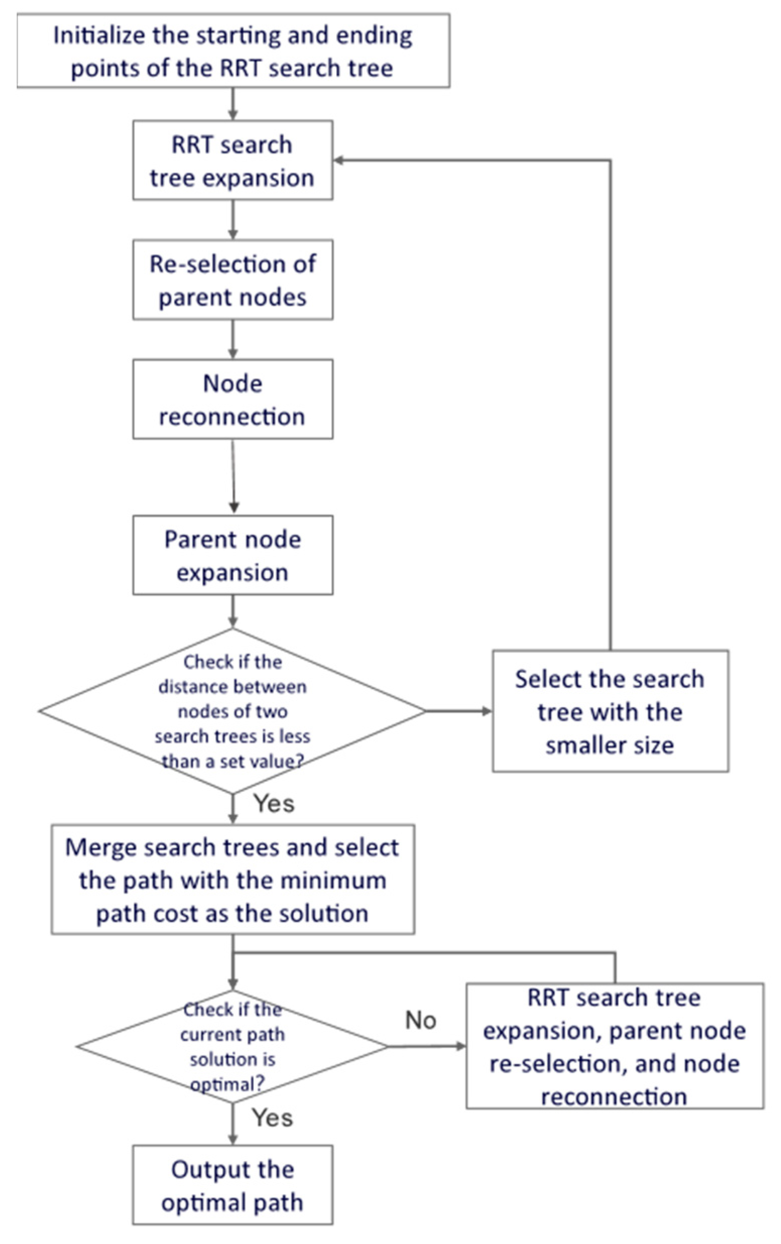
To visualize the execution logic of the classical B-RRT* algorithm, Figure 5 presents its procedural flowchart. The algorithm initiates by initializing the starting and ending points of the RRT search tree. It then proceeds with RRT search tree expansion to grow the tree structure. Next, re-selection of parent nodes optimizes node connections, followed by node reconnection to refine the tree topology. Parent node expansion further extends the tree, after which a check verifies if the distance between nodes of two search trees falls below a preset threshold. If true, the search trees merge, and the path with the minimum cost is selected as a candidate solution. A subsequent check assesses if this path is optimal; if not, the process loops back to RRT search tree expansion, parent node re-selection, and node reconnection. When the optimal path is confirmed, it is output. Notably, during tree expansion, the algorithm selects the search tree with the smaller size to balance bidirectional growth, a key feature of bidirectional RRT variants. This flowchart encapsulates the classical B-RRT*’s core steps—tree expansion, node optimization, bidirectional merging, and optimality verification—providing a baseline for comparing it with the improved B-RRT* algorithm (presented in Figure 6).

To enhance the path-planning efficiency of the B-RRT* algorithm, this paper incorporates adaptive Gaussian distribution sampling and dynamic goal biasing into the original algorithm. Adibeli et al. proposed a modified Bi-RRT* algorithm with variable node parameters for nuclear decommissioning environments—by classifying nodes into quarter/half/full types and performing customized operations (e.g., parent selection, rewiring), they improved path optimality and computational efficiency; this node-oriented optimization idea provides a reference for the improved B-RRT* algorithm in this paper to optimize sampling and expansion based on environmental characteristics [25]. The flowchart of the improved B-RRT* algorithm is illustrated in Figure 6.

The overall procedure of the improved B-RRT* is summarized in Algorithm 1. Compared with the classical B-RRT*, the proposed method integrates adaptive Gaussian sampling and dynamic target biasing, which guide the sampling process toward promising regions while avoiding obstacles.

Algorithm 1 Improved B-RRT*

1: Input Start point $x_{\mathrm{start}}$, goal point $x_{\mathrm{goal}}$, map space $X$, obstacle space $X_{\mathrm{obs}}$, step size $\delta$, maximun iterations $N$, bias weight $\mathrm{\gamma }$ 2: Output Optimized path $\mathcal{P}$ 3: Initialize two trees: $T_{start}$ and $T_{\mathrm{goal}}$ 4: Add $X_{start}$ to $X_{goal}$ and $T_{start}$ to $T_{\mathrm{goal}}$ 5: Set bias threshold $Q$ 6: $\mathcal{P}\leftarrow \mathrm{\varnothing }$ 7: for $K=1$ to $N$ do 8:   Adaptive Sampling 9:   Generate $p\sim U\left(0,1\right)$ 10:    if $p\le Q$ then 11:    $q_{rand}\leftarrow x_{goal}$ 12:    else 13:    Compute Gaussian mean $\mu$ based on current node and target 14:    Define obstacle weight functions:         ${\mathrm{\omega }}_{\mathrm{out}}\left(c\right)=\mathrm{e}\mathrm{x}\mathrm{p}\left(-{\displaystyle \frac{d\left(c,O\right)}{2{\mathrm{\sigma }}^2}}\right),\hspace{1em}{\mathrm{\omega }}_{\mathrm{o}\mathrm{u}\mathrm{t}}\left(\mathrm{c}\right)=\mathrm{e}\mathrm{x}\mathrm{p}\left(-{\displaystyle \frac{\mathrm{d}\left(\mathrm{c},\mathrm{O}\right)}{2{\mathrm{\sigma }}^2}}\right)$ 15:    Generate $q_{\mathrm{rand}}$ using weighted Gaussian distribution 16:    end if 17:    Nearest Neighbor Search: 18:    Find $q_{\mathrm{nearest}}\in \mathcal{T}$ closest to $q_{rand}$ 19:    Steer and Collision Check: 20:    Generate $q_{new}$ by moving from $q_{nearest}$ toward $q_{rand}$ with step size $\delta$ 21:    if $q_{new}ϵX\backslash X_{obs}$ then 22:    Add $q_{new}$ to tree 23:    end if 24:    Parent Selection and Rewiring: 25:    Choose parent of $q_{new}$ minimizing path cost 26:    Rewire nearby nodes if cost is reduced 27:    Dynamic Target Bias Adjustment: 28:    Update $Q$:            $Q=\left[{\gamma ·Q}_1+\left(1-\gamma \right)·Q_2\right]$/2, $Q_1={\displaystyle \frac{1}{1+\alpha \cdot e^{-\beta \cdot h}}}$ , $Q_2={\left(1-{\displaystyle \frac{S}{\pi ·{step}^2}}\right)}^2+t$ 29:    Tree Connection: 30:    if exists $q\in {\mathcal{T}}_{goal}$ such that $‖q_{new}-q‖<\delta$ then 31:    Merge ${\mathcal{T}}_{start}$ and ${\mathcal{T}}_{goal}$ 32:    Compute path cost 33:    end if 34:    if valid path found then 35:    Extract minimum cost path $\mathcal{P}$ 36:    break 37:    end if 38: end for 39: Return: $\mathcal{P}$

In Algorithm 1, Adaptive sampling and Dynamic Target Bias Adjustment are the main improvements. Adaptive sampling adjusts the Gaussian distribution by obstacle-related weights, thereby reducing invalid samples. Dynamic Target Bias Adjustment updates the goal bias probability Q according to obstacle density and target distance, improving convergence efficiency.

The improved B-RRT* algorithm optimizes the random tree expansion process through adaptive sampling and dynamic bias, which is consistent with the node classification idea proposed by Xiong et al. in the Classified-RRT* algorithm—they classified nodes based on connectivity with start/goal points and performed customized Choose Parent and Rewire procedures, significantly improving convergence rate and path quality. Similarly, this paper’s improved B-RRT* algorithm adjusts sampling and expansion strategies according to obstacle density and target distance, achieving similar optimization effects in warehouse environments [26]. To verify the performance of the improved B-RRT* algorithm in both simple and complex environments, two sets of simulation experiments were designed. One used a complex environment map, and the other a simple one. The hardware setup comprised 16 GB of memory and an AMD Ryzen7 5800H processor, with Python 3.9.3 as the software environment.

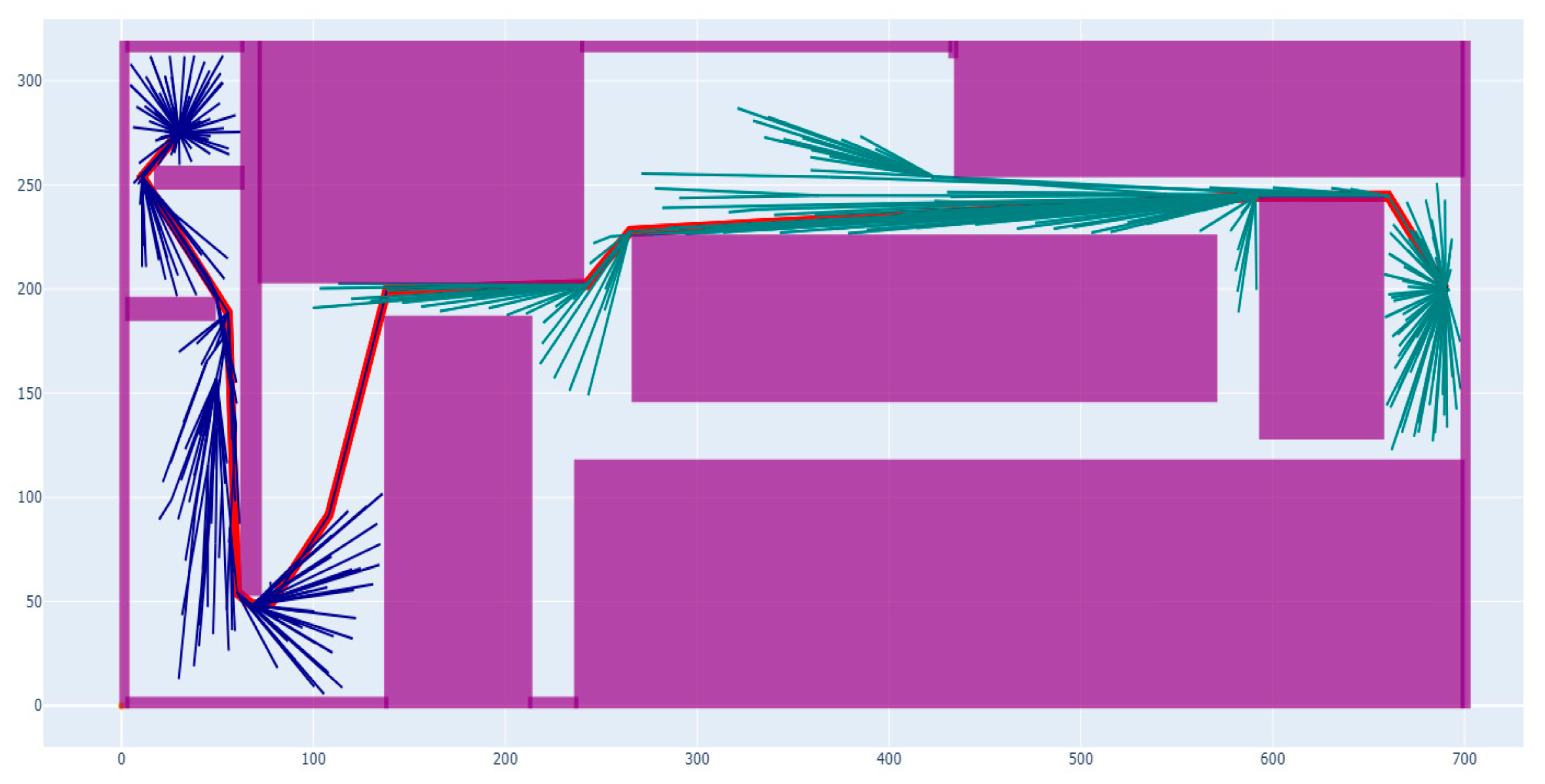
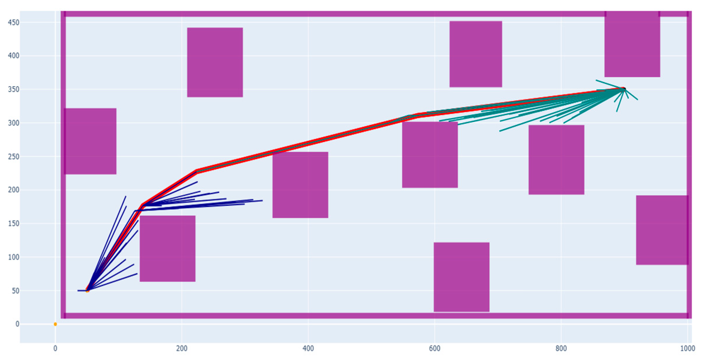
To evaluate the algorithm’s performance in complex obstacle-filled settings, a maze-like environment with large-scale obstacles was designed. Figure 7 and Figure 8 show the path-planning outcomes for the original and improved B-RRT* algorithms, respectively. In the figure, the obstacles are shown in purple, and the searched paths are shown in trees, as blue and green lines, respectively.

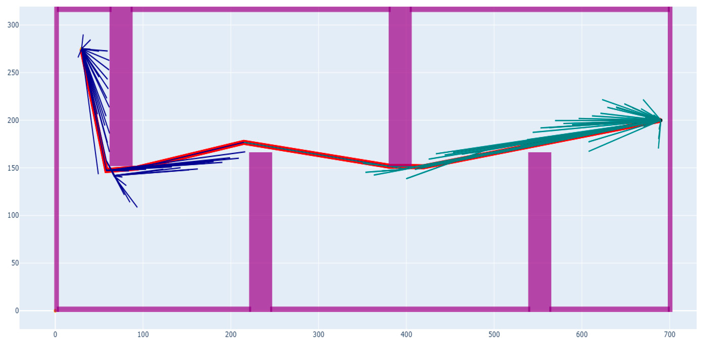
In order to verify the performance of the algorithm in a simple obstacle environment, a typical scenario containing four small obstacles is designed. Figure 9 and Figure 10 show the path-planning results of the initial B-RRT* algorithm and the improved B-RRT* algorithm, respectively.

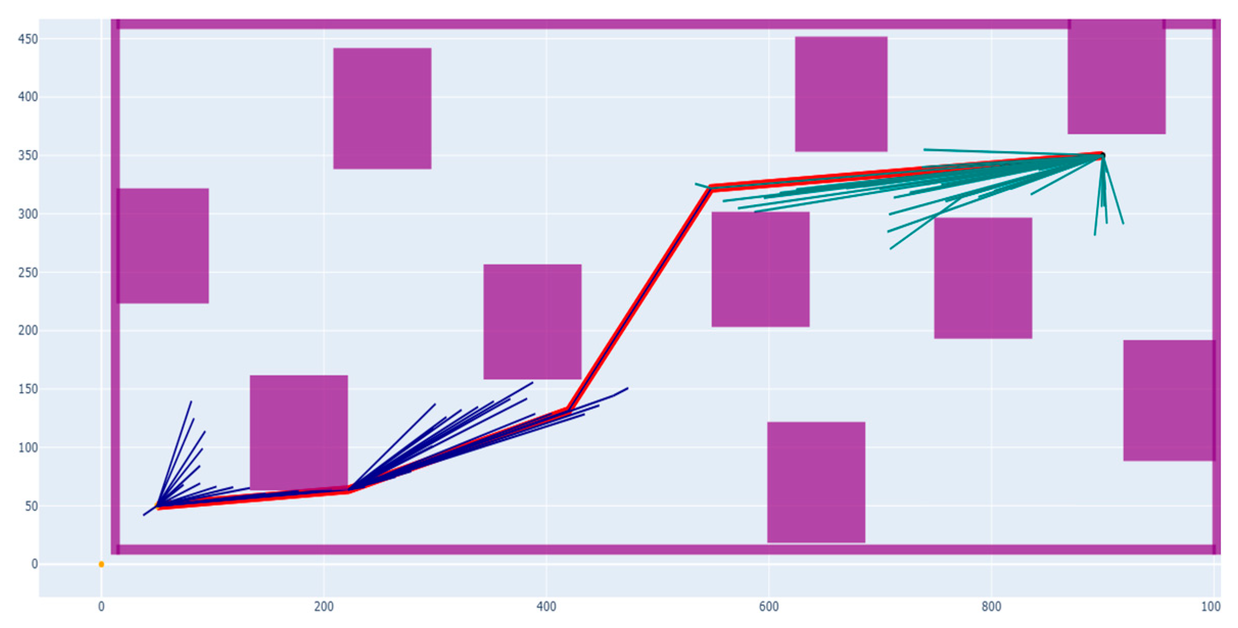
In order to verify the performance of the algorithm in an irregular obstacle environment, a typical scenario containing 10 obstacles is designed. Figure 11 and Figure 12 show the path-planning results of the initial B-RRT* algorithm and the improved B-RRT* algorithm, respectively.

By analyzing the experimental results, it can be seen that the initial B-RRT* algorithm, due to the random sampling method, leads to too scattered sampling points. This is especially true when the environment is complex: there are too many invalid sampling points, which affects the search efficiency of the algorithm, and there are too many path turning points. The improved B-RRT* algorithm introduces Gaussian distribution sampling and a dynamic target bias strategy to guide the sampling points, which makes the generation of sampling points more purpose-based, reduces the generation of unnecessary sampling points, improves the search efficiency of the algorithm, and verifies the effectiveness of the algorithm.

To ensure the reliability and statistical significance of the experimental results, 10 repeated experiments were conducted for each of the three types of environment maps (complex, simple, and irregular), and the average values of key performance indicators (operation time, path length, and number of sampling points) from the 10 experiments were used as the final data for comparison. In the experimental test with a complex environment, compared with the original B-RRT* algorithm, the path length of the improved B-RRT* algorithm is reduced by 14.4%, the operation time is reduced by 26.8%, and the number of sampling points is reduced by 37.6%. In the experimental test with a simple environment, compared with the original B-RRT* algorithm, the improved B-RRT* algorithm reduces the path length by 9.8%, the operation time by 21.3%, and the number of sampling points by 30.7%. Moreover, in the experimental test with an irregular environment, compared with the original B-RRT* algorithm, the improved B-RRT* algorithm reduces the path length by 4.6%, the operation time by 22.5%, and the number of sampling points by 16.1%. Overall, the improved B-RRT* algorithm has been tested in complex, simple and irregular environments, and compared with the original B-RRT* algorithm, it has an improved search efficiency, number of effective sampling points, and path quality, and the effect is more significant in the complex environment. Each algorithm was tested with 100 runs in each environment to test its success rate. The test results are shown in

Table 1. Comparison results of algorithms in different environments.

Environment	Algorithm	Operation Time/s	The Path Length/m	Number of Sampling Points	Operation Success Rate
Complex	B-RRT*	3.76	57.76	861	93%
	Improving B-RRT*	2.75	50.49	537	95%
Easy	B-RRT*	1.03	42.02	299	100%
	Improving B-RRT*	0.81	38.27	207	100%
Irregularity	B-RRT*	0.62	49.62	156	100%
	Improving B-RRT*	0.48	47.33	186	100%

.

2.3. Charging Scheduling Strategy and Model Construction Under Multiple Charging Points

2.3.1. Description of the Charging Scheduling Problem for Multiple Charging Points

For large warehouses, when the number of inspection tasks is large and the layout is scattered, even a mobile robot with full power cannot complete all inspection tasks at once without charging. During the inspection, the power must be replenishable at the charging point to support the completion of subsequent inspection tasks. In particular, when the inspection task is far away from the charging point or the inspection task takes a long time and consumes a lot of power, even a mobile robot with full power cannot complete the overall process of moving from the charging point to the task point, processing the task, and returning from the task point to the charging point. Therefore, it is necessary to set up multiple charging points based on the warehouse environment and task conditions to supplement the power of the robot in the middle of the task. In addition, multiple charging points are set up in different areas of the warehouse. The robot can choose appropriate charging points in different areas of the warehouse, reducing unnecessary round trips and power consumption during recharging. In summary, it is necessary and of certain practical significance to study the path-planning problem of mobile robot warehouse inspection under the condition of multiple charging points.

This paper aims to minimize the electricity consumption of the robot, denoted as C, which satisfies the following equation:

$$C=C_{path}+C_{task}$$

(12)

The power consumption of the robot has two parts, where $C_{path}$ is the power consumption of the robot in the process of warehouse inspection, and $C_{task}$ is the power consumption of the robot needed to complete all patrol tasks, set to $C_{task}$.

Since $C_{task}$ is a fixed value, minimizing C is equivalent to minimizing $C_{path}$. In the ideal case, it can be considered that each unit of electricity supports the robot to move the same distance, and the final robot charging scheduling problem is transformed into a path-planning problem to minimize the mobile path length of the robot inspection process.

2.3.2. Charging Scheduling Planning for Multiple Charging Points

Before the path planning of the robot considering charging scheduling under multiple charging points, we need to set the charging scheduling rules of the robot. In general, the charging scheduling rule mainly considers three points: (1) when to charge, (2) which charging point to choose, and (3) how full the charge is. For the problem in this paper, the amount of charge has no effect on power consumption, and the rule mainly affects the charging time. If a robot’s remaining power is sufficient to complete the next inspection task (including moving to the task point and returning to a charging point), it does not require full charging. Specifically, when the sum of the power needed for the remaining task and the round-trip movement is less than the robot’s total capacity, partial charging is sufficient. In the limit, it only needs to be charged to the required power value. But time is not our goal in this problem. Rules (1) and (2) have a practical impact on the path. When to charge will affect the situation of optional charging points, and the choice of charging points will affect the actual path. Therefore, there are two rules to be determined finally:

• Study which inspection task the robot will complete before going to the charging point.
• When the robot is ready to charge, we should study which charging point the robot chooses to supplement its power.

For the problem of when to charge the robot, we set a strategy that when the robot arrives at a task site each time and completes the task, it will judge whether its remaining power can support it to complete the overall process of arriving at the next task site, completing the task, and returning to the charging point closest to the task site. If it is shown that the remaining power is not sufficient to support the robot to achieve the process of reaching the task point, completing the task, and charging, then it is necessary to find a charging point for charging.

In view of the problem of which charging point the robot chooses, the charging point closest to the current position is generally selected, which is a sound strategy to ensure that the robot starts charging in the shortest time. However, this is not the best strategy, because this strategy is similar to the greedy strategy, which only considers the present without considering the future, and in some cases it will deviate from the current route. Therefore, we improve this strategy. When charging is needed, we select the closest charging point to the next task that can be supported by its remaining power, while also considering the location of the next task to ensure sufficient power for its completion. It can effectively reduce the overall inspection path process.

Figure 13 shows the overall process of charging scheduling in this paper:

2.3.3. Model Building

The global path planning in this paper mainly solves the charging scheduling problem in the case of considering the power limit and there are multiple charging points. In order to solve this problem, it is necessary to construct a charging scheduling model under multiple charging points. The notation definitions used in the mathematical model are given below, as shown in

Table 2. Definition of mathematical model notation.

Symbol	Symbol Description
$C_{path}$	The total power consumption of the path in the inspection process
$m_i$	Patrol the power consumed by task i
$d_{ij}$	Power consumption from patrol task i to patrol task j, where i ≠ j
$e_{ci,j}$	Power consumption from charging point i to patrol task j
$e_{j,ci}$	$\mathrm{The}\mathrm{power}\mathrm{consumption}\mathrm{from}\mathrm{inspection}\mathrm{task}\mathrm{j}\mathrm{to}\mathrm{charging}\mathrm{point}\mathrm{i}\mathrm{is}\mathrm{equal}\mathrm{to}{e}_{ci,j}$
$e_{ci,cj}$	Power consumption from charging point i to charging point j
$x_{ij}$	Equal to 1 when the robot moves from patrol task i to patrol task j, and 0 otherwise, where i ≠ j
$y_{ci,j}$	It is equal to 1 when the robot moves from charging point i to inspection task j, and 0 otherwise
$y_{j,ci}$	It is equal to 1 when the robot moves from patrol task j to charging point i, and 0 otherwise
$z_{ci,cj}$	It is equal to 1 when the robot moves from charge point i to charge point j, and 0 otherwise
$N$	Collection of inspection points
$P$	Set of charging points, where charging point 0 is the start and end point of the inspection
$R_{i,ar}$	The remaining power at inspection task point i
$R_{i,le}$	The remaining power to complete inspection task i
$R_{ci}$	The remaining amount of power to reach charging point i

.

Firstly, the following basic assumptions are made for the mobile robot charging scheduling problem in this paper:

• The mobile robot with full power has 100 units of power, and the power consumption of each inspection task and the power consumption from one inspection task to the next inspection task are based on unit power.
• The moving speed of the robot is constant, and it takes the same time to consume each unit of electricity during the moving process.
• The charging rate of each charging point is the same, and the time to replenish each unit of power consumption is the same.
• For the convenience of management, the robot starts the inspection task from a fixed charging point and returns to the charging point after the inspection task is finished.
• When the robot reaches the charging point, it will not leave until the battery is full.
• When the charging point is set reasonably, it is considered that there is no repeat access to the charging point, and there is no movement from one charging point to the charging point.

The objective function of the mathematical model is as follows:

$$min{C}_{path}={\sum }_{i\in N}{\sum }_{j\in N}{x}_{ij}{d}_{ij}+{\sum }_{i\in P}{\sum }_{j\in N}{y}_{ci,j}{e}_{ci,j}+{\sum }_{i\in N}{\sum }_{j\in P}{y}_{i,cj}{e}_{i,cj}$$

(13)

There are two kinds of constraints, namely path constraints and quantity constraints.

The node access restriction constraint is described as

$${\sum }_{i\in N}{x}_{ij}+{\sum }_{i\in P}{y}_{ci,j}=1j\in N$$

(14)

$${\sum }_{j\in N}{x}_{ij}+{\sum }_{j\in P}{y}_{i,cj}=1i\in N$$

(15)

$${\sum }_{j\in N}{y}_{c0,j}=1$$

(16)

$${\sum }_{i\in N}{y}_{i,c0}=1$$

(17)

Constraint (14) means that the inspection task j can only be reached once. Constraint (15) means that the terminal charging point can only be reached once. Constraint (16) means arriving at a patrol task point or charging point from the starting charging point; Constraint (17) means returning to the starting charging point from the charging point or the patrol task point.

The subloop limiting constraints are

$${\mu }_i-{\mu }_j+N{x}_{ij}\le N-11<i\ne ji,j\in N$$

(18)

$${\beta }_{ci}-{\beta }_j+N{y}_{ci,j}\le N-1j>1i\in P,j\in N$$

(19)

$${\beta }_i-{\beta }_{cj}+N{y}_{i,cj}\le N-1i>1i\in N,j\in P$$

(20)

$${\beta }_{ci}-{\beta }_{cj}+N{z}_{ci,cj}\le N-1i,j\in P$$

(21)

where μ and β are auxiliary variables with values greater than 0, and N is the sum of the number of tasks and the number of charging points.

The quantity constraint is

$$R_{i,le}=R_{i,ar}-m_{i}i\in N$$

(22)

$$x_{ij}\left(R_{i,le}-{R_{j,ar}-d}_{ij}\right)=0i\in N,j\in N,i\ne j$$

(23)

$$y_{ci,j}\left(100-R_{j,ar}-e_{ci,j}\right)=0i\in N,j\in N,i\ne j$$

(24)

$$y_{i,cj}\left(R_{i,le}-R_{cj}-e_{i,cj}\right)=0i\in N,j\in N,i\ne j$$

(25)

Constraint (22) represents the change in electricity quantity between task point i and task point i. Constraint (23) represents the change in the amount of electricity when the robot arrives at task j after task i is completed. Constraint (24) represents the change in the amount of electricity arriving at task j after the robot leaves charging point i; Constraint (25) represents the change in the amount of electricity in the robot arriving at charging point j after its departure from task i.

3. Results

3.1. Experimental Environment

All cases in this paper are run in the hardware environment of AMD Ryzen7 5800H CPU, RTX 3060 graphics card, 16GB memory, Windows 11 operating system, pycharm running software, and Python version 3.9.7. Because the algorithm used for local path planning is a random algorithm based on sampling, there are inevitably accidents in the simulation experiment process. In order to ensure the reliability of the experimental results, five independent simulation experiments are carried out for each map, and all the experimental results are compared and analyzed.

3.2. Simulation Verification

In order to verify the feasibility of the research model, a case study is carried out according to the model and algorithm specified in Chapter III and Chapter IV, as well as the raster map. Gurobi is used to solve the case, and the maximum relative gap value is 10%. In the local path planning, the improved B-RRT* algorithm is compared with the initial B-RRT* algorithm and RRT* algorithm. The number of sample points is set to 1000, the step size of the expansion tree is set to divide the minimum length and width of the map by 30 and then round down, and the number of node reconnections is 50. In the global path planning, the number of iterations is set to 200. The maps of four different warehouse environments are set, where case 1 is a scene with wide space and regular obstacle placement, case 2 is a scene with narrow space and regular obstacle placement, case 3 is a scene with narrow space and irregular obstacle placement, and case 4 is a scene with wide space and irregular obstacle placement. Additionally, 20, 40, and 60 task points to be checked and a number of charging points are randomly set where there are no obstacles, and five experiments are performed each time to obtain the average value. The inspection process requires the completion of all inspection tasks starting from the charging pile and then returning to the charging pile.

-

Case 1:

In a complex scene with regular obstacles, a wide space, multi-corridor structure and uneven distribution of task points (task points, charging points, and obstacles are represented by black dots, green icons and purple squares, respectively, in the figure), the path color changes after each charging of the robot, which intuitively reflects the relationship between charging behavior and path switching. This experiment systematically compares the performance of the proposed improved B-RRT algorithm with the traditional RRT and initial B-RRT algorithms. The results of the experiment are shown in Figure 14, Figure 15 and Figure 16, and the experimental data are shown in

Table 3. Case 1 scheduling consumption of different task points.

Types of Local Algorithms	Number of Mission Points	Average Local Solution Time ${\mathit{t}}_1$/s *	Average Number of Sampling Points	Average Global Solution Time ${\mathit{t}}_2$/s **	Average Total Path Cost
RRT*	20	24.239	389	1.016	114.369
Initial B-RRT*		8.730	179	1.038	113.334
Improved B-RRT*		7.591	146	0.989	103.977
RRT*	40	126.519	715	38.955	178.494
Initial B-RRT*		48.901	300	39.887	171.289
Improved B-RRT*		42.522	235	37.988	156.001
RRT*	60	405.682	849	101.659	248.489
Initial B-RRT*		149.658	302	104.586	242.460
Improved B-RRT*		133.624	256	99.586	219.819

* Local path-planning time. ** Global path-planning time.

.

Experimental results show that the improved B-RRT is significantly better than the comparison algorithms in a number of key indicators, showing excellent comprehensive performance. For example, under the scale of 60 task points, the solving time of the algorithm is 133.624 s, which is 67.1% lower than the 405.682 s of RRT*, and 10.7% lower than the 149.658 s of initial B-RRT*. In terms of sampling efficiency, the improved B-RRT only needs 235 sampling points in the environment with 40 task points, which is 67.1% less than the 715 sampling points of RRT and 21.7% less than the 300 sampling points of initial B-RRT, reflecting better search ability and convergence. In terms of path quality, the path cost of the proposed method is 103.977 under the scale of 20 task points, which is 9.1% lower than the 114.369 of RRT and 8.3% lower than the 113.334 of initial B-RRT*, indicating that the planned path has higher economy. In addition, the improved B-RRT* integrated with the charging scheduling model not only effectively generates feasible patrol task scheduling schemes but also has the ability to identify redundant charging stations, which provides a theoretical basis and decision support for the optimal deployment of charging infrastructure in the actual system. The results fully verify that the algorithm has good generalization ability, robustness, and practical application value in complex environments.

-

Case 2:

In the case of narrow space, narrow channels and regular obstacle placement (the task point, charging point, and obstacle are represented by black points, green icons and purple squares, respectively, in the figure), the path color of the robot changes after each charge, which intuitively reflects the relationship between charging behavior and path switching. This experiment systematically compares the performance of the proposed improved B-RRT algorithm with the traditional RRT and initial B-RRT algorithms. The results of the experiment are shown in Figure 17, Figure 18 and Figure 19, and the experimental data are shown in

Table 4. Case 2 scheduling consumption of different task points.

Types of Local Algorithms	Number of Mission Points	Average Local Solution Time ${\mathit{t}}_1$/s *	Average Number of Sampling Points	Average Global Solution Time ${\mathit{t}}_2$/s **	Average Total Path Cost
RRT*	20	56.369	389	1.106	168.569
Initial B-RRT*		24.512	197	1.031	162.350
Improved B-RRT*		20.017	164	0.983	154.619
RRT*	40	186.652	468	24.205	189.657
Initial B-RRT*		85.623	252	23.062	184.487
Improved B-RRT*		69.849	224	21.964	175.702
RRT*	60	462.145	715	85.694	206.215
Initial B-RRT*		188.497	292	83.977	197.393
Improved B-RRT*		171.361	243	79.978	187.993

* Local path-planning time. ** Global path-planning time.

.

Experimental results show that the improved B-RRT is significantly better than the comparison algorithms in a number of key indicators, showing excellent comprehensive performance. For example, under the scale of 60 task points, the solving time of the algorithm is 171.361 s, which is 62.9% lower than that of RRT* (462.145 s), and 9.1% lower than that of initial B-RRT* (188.497 s). In terms of sampling efficiency, the improved B-RRT only needs 224 sampling points in the environment of 40 task points, which is 52.1% less than RRT’s 468 sampling points and 11.1% less than initial B-RRT’s 252 sampling points, reflecting better search ability and convergence. In terms of path quality, the path cost of the proposed method is 154.619 under the scale of 20 task points, which is 8.3% lower than that of RRT (168.569) and 4.8% lower than that of initial B-RRT* (162.350), indicating that the planned path has higher economy. In reality, the shelves of many warehouses are placed closely and the styles are various. The results fully verify that the algorithm has good practical application value in complex environments.

-

Case 3:

In the case of narrow space, irregular placement of obstacles and uneven distribution of channel width (in the figure, task points, charging points and obstacles are represented by black points, green icons and purple squares, respectively), the color of the robot path changes after each charge, which intuitively reflects the relationship between charging behavior and path switching. This experiment systematically compares the performance of the proposed improved B-RRT algorithm with the traditional RRT and initial B-RRT algorithms. The results of the experiment are shown in Figure 20, Figure 21 and Figure 22, and the experimental data are shown in

Table 5. Case 3 scheduling consumption of different task points.

Types of Local Algorithms	Number of Mission Points	Average Local Solution Time ${\mathit{t}}_1$/s *	Average Number of Sampling Points	Average Global Solution Time ${\mathit{t}}_2$/s **	Average Total Path Cost
RRT*	20	83.654	596	3.235	135.594
Initial B-RRT*		31.642	424	3.121	132.547
Improved B-RRT*		26.368	319	2.972	123.932
RRT*	40	189.652	769	31.236	191.641
Initial B-RRT*		90.414	471	31.479	188.005
Improved B-RRT*		75.345	356	29.980	176.949
RRT*	60	568.954	804	186.669	206.364
Initial B-RRT*		219.574	497	184.885	203.839
Improved B-RRT*		182.978	374	176.081	192.395

* Local path-planning time. ** Global path-planning time.

.

Experimental results show that the improved B-RRT is significantly better than the comparison algorithms in a number of key indicators, showing excellent comprehensive performance. For example, under the scale of 60 task points, the solving time of the algorithm is 182.978 s, which is 67.8% lower than that of RRT* (568.954 s), and 16.7% lower than that of initial B-RRT* (219.574 s). In terms of sampling efficiency, improved B-RRT only needs 356 sampling points in the environment of 40 task points, which is 53.7% less than the 769 sampling points of RRT and 24.4% less than the 471 sampling points of initial B-RRT, reflecting better search ability. In terms of path quality, the path cost of the proposed method is 123.932 under the scale of 20 task points, which is 8.6% lower than that of RRT (135.594) and 6.5% lower than that of initial B-RRT* (132.547), indicating that the planned path has higher economy. This case can be extended to large-scale inspection tasks inside the factory, when the scale of obstacles is different and the tasks are distributed in different areas. The improved B-RRT* integrated with the charging scheduling model not only effectively generates feasible patrol task scheduling schemes, but also has the ability to identify redundant charging stations, which provides a theoretical basis and decision support for the optimal deployment of charging infrastructure in the actual system. The results fully verify the practical application value of the algorithm in complex environments.

-

Case 4:

In the face of a complex environment, especially when the shelves are relatively cluttered, the paths are complex, and the task points to be inspected are dense and randomly distributed (the task points, charging points and obstacles are represented by black dots, green icons and purple squares, respectively, in the figure), the path color of the robot changes after each charge, which intuitively reflects the relationship between charging behavior and path switching. This experiment systematically compares the performance of the proposed improved B-RRT algorithm with the traditional RRT and initial B-RRT algorithms. The results of the experiment are shown in Figure 23, Figure 24 and Figure 25, and the experimental data are shown in

Table 6. Case 4 scheduling consumption of different task points.

Types of Local Algorithms	Number of Mission Points	Average Local Solution Time ${\mathit{t}}_1$/s *	Average Number of Sampling Points	Average Global Solution Time ${\mathit{t}}_2$/s **	Average Total Path Cost
RRT*	20	61.173	295	2.234	149.155
Initial B-RRT*		21.783	181	2.122	135.947
Improved B-RRT*		18.942	157	2.021	129.473
RRT*	40	193.087	389	22.658	170.927
Initial B-RRT*		60.154	240	23.107	173.948
Improved B-RRT*		52.308	209	22.007	164.712
RRT*	60	228.727	759	59.236	209.592
Initial B-RRT*		106.925	389	59.880	211.589
Improved B-RRT*		92.978	338	57.028	201.513

* Local path-planning time. ** Global path-planning time.

.

Experimental results show that the improved B-RRT is significantly better than the comparison algorithms in a number of key indicators, showing excellent comprehensive performance. For example, under the scale of 60 task points, the solving time of the algorithm is 92.978 s, which is 59.4% lower than that of RRT* (228.727 s), and 13.0% lower than that of initial B-RRT* (106.925 s). In terms of sampling efficiency, improved B-RRT only needs 209 sampling points in the environment of 40 task points, which is 46.3% less than the 389 sampling points of RRT and 12.9% less than the 240 sampling points of initial B-RRT, reflecting better search ability and convergence. In terms of path quality, the path cost of the proposed method is 129.473 under the scale of 20 task points, which is 13.2% lower than that of RRT (149.155) and 4.8% lower than that of initial B-RRT* (135.947), indicating that the planned path has higher economy. The results fully verify that the algorithm has good generalization ability and practical application value in complex environments. It has value for facing the harsh environment of warehouses.

To ensure the reliability of the results, paired t-tests were applied to compare the performance of the improved B-RRT* against RRT* and initial B-RRT*. The tests confirm that the differences in path length, computation time, and number of sampling points are statistically significant in all environments (p < 0.05).

4. Discussions

• The optimization model considers the power supply problem in the face of multi-task points, and sets up charging points in the appropriate locations to make the model closer to the actual operation situation. Before the robot dog plans its path according to the tasks to be inspected, it will give priority to the current battery power reserve, the consumption cost during the execution of the task, and the consumption cost during the execution of the task. After the execution of a task, when its own power cannot be used to reach the next task, it will give priority to the nearest charging point, and then re-plan the path until all the tasks to be carried out can be covered. The optimal path-planning scheme with the minimum total cost and satisfying charging demands was formed. It should be noted that in this study, the charging stations were distributed uniformly according to the warehouse layout, which occasionally led to redundant stations. Optimizing the number and placement of charging stations is beyond the scope of this paper but represents an important direction for future research, which could be addressed using facility location models or heuristic optimization methods.
• In different scale test scenarios, from a small number of inspection points to a large number of complex distributed inspection points, the model shows good solution speed. To ensure that the performance gains are not the result of random variations inherent in sampling-based algorithms, we conducted paired t-tests across 10 independent runs for each scenario. The results show that the differences between the improved B-RRT* and the baseline algorithms are statistically significant in terms of all three performance metrics (p < 0.05). This confirms that the observed improvements are robust and reliable, rather than coincidental. For the scene containing 20 task points to be inspected, the longest solution time is 29.59 s, and the average solution time is about 20.93 s according to the complexity of the map. As the scale of the scene increases to a medium scale (40 or 60 task points to be inspected), the solving time increases, but it can still be controlled in a reasonable range, and the average time of 40 task points is about 88.09 s. For 60 task points, due to the number of task points being too high and some maps being more complex, the solution time is 233.95 s. With the increase in map complexity, the solution time also increases slightly, but it is also far lower than the solution time of traditional path-planning algorithms in similar scenarios. Additional experiments showed that the improved B-RRT* is robust to parameter variations: while step size, number of samples, and bias weight influence the trade-off between efficiency and path quality, the algorithm consistently outperforms the baselines across a wide range of settings.
• The path-planning model and solution results have strong adaptability in the actual robot dog inspection scene. By modifying the battery capacity, power consumption during task execution and path cost, the number and location of inspection points and the location of charging points can be set, the factory inspection environment can be simulated, and the order of inspection points can be reasonably arranged to meet the requirements of inspection tasks under different circumstances. From the cost–benefit point of view, this path-planning scheme has significant application value. By optimizing the path planning, the invalid walking distance of the robot dog is reduced and the energy consumption is reduced. This not only prolongs the working time of the robot dog after a single charge and reduces the number of charges, but also reduces the equipment loss and maintenance cost caused by frequent charging, and efficient path planning improves the inspection efficiency, meaning inspection tasks can be completed in a shorter time, indirectly bringing the improvement of economic benefits.

5. Conclusions

In this paper, a warehouse simulation map model is established based on a grayscale map. Combined with the remaining tasks in the scheduling process and the distance between charging points and other elements, the general charging scheduling rules are improved. For the path-planning problem of warehouse patrol charging scheduling, considering power limits under multiple charging points, this paper divides the problem into two parts: local path planning to solve the path cost matrix between charging points and patrol task points, and global path planning to solve the charging scheduling sequence.

In the local path planning, we propose an improved B-RRT* algorithm that integrates adaptive Gaussian distribution sampling and a dynamic target bias strategy. This approach guides the sampling points toward the target region, reduces invalid search ranges, and significantly enhances search efficiency. Experimental results demonstrate that the improved B-RRT* algorithm achieves an average reduction of 10–15% in path length, 20–30% in computation time, and 15–40% in the number of sampling points compared to the original B-RRT* and RRT* algorithms across various warehouse environments.

In the global path planning, a mixed integer programming model for mobile robot inspection and charging scheduling under multiple charging points is established, solved efficiently using the Gurobi solver. Case studies with 20, 40, and 60 patrol tasks show that the proposed model can generate feasible and efficient charging schedules within reasonable timeframes, even in large-scale and complex scenarios.

In summary, the improved B-RRT algorithm not only enhances local path-planning efficiency and quality but also, when integrated with the charging scheduling model, provides a practical and robust solution for autonomous warehouse inspection under power constraints. The method demonstrates strong applicability and scalability, offering significant value for real-world deployment.

References

1. Pei, Z.; Wan, M.; Du, R.; Li, Y.; Chen, Y. Charging scheduling considering the release time of carrying machinery under multiple charging piles. Comput. Integr. Manuf. Syst. 2021, 4, 1089–1098. (In Chinese) [Google Scholar]
2. Ravankar, A.; Ravankar, A.A.; Watanabe, M.; Hoshino, Y.; Rawankar, A. Multi-robot path planning for smart access of distributed charging points in map. Artif. Life Robot. 2021, 26, 52–60. [Google Scholar] [CrossRef]
3. Hao, B.; Du, H.; Dai, X.; Liang, H. Automatic recharging path planning for cleaning robots. Mob. Inf. Syst. 2021, 2021, 5558096. [Google Scholar] [CrossRef]
4. Li, Z. Research on Path Planning Problem of Electric Logistics Vehicle Considering Different Power Supply Modes. Ph.D. Thesis, Shenyang University of Technology, Shenyang, China, 2021. (In Chinese). [Google Scholar]
5. Yuan, J. Research on Electric Bus Driving Plan Considering Charging Continuity and Demand Response. Ph.D. Thesis, Shenyang University of Technology, Shenyang, China, 2023. (In Chinese). [Google Scholar]
6. Alizadeh, M.; Wai, H.T.; Scaglione, A.; Goldsmith, A.; Fan, Y.Y.; Javidi, T. Optimized path planning for electric vehicle routing and charging. In Proceedings of the 2014 52nd Annual Allerton Conference on Communication, Control, and Computing (Allerton), Monticello, IL, USA, 30 September–3 October 2014; IEEE: New York, NY, USA, 2014; pp. 25–32. [Google Scholar]
7. Duchoň, F.; Babinec, A.; Kajan, M.; Beňo, P.; Florek, M.; Fico, T.; Jurišica, L. Path planning with modified a star algorithm for a mobile robot. Procedia Eng. 2014, 96, 59–69. [Google Scholar] [CrossRef]
8. Noreen, I.; Khan, A.; Habib, Z. Optimal path planning using RRT* based approaches: A survey and future directions. Int. J. Adv. Comput. Sci. Appl. 2016, 7, 97–107. [Google Scholar] [CrossRef]
9. Wang, H.; Yu, Y.; Yuan, Q. Application of Dijkstra algorithm in robot path-planning. In Proceedings of the 2011 Second International Conference on Mechanic Automation and Control Engineering, Inner Mongolia, China, 15–17 July 2011; IEEE: New York, NY, USA, 2011; pp. 1067–1069. [Google Scholar]
10. Zhang, T.; Li, Q. Mobile robot path planning based on B-RRT * FND algorithm. Control. Decis. 2023, 11, 3121–3127. (In Chinese) [Google Scholar]
11. Meng, W.L.; Pu, Y.B.; Gong, Y. Fusion of local–global strategy for AUV path planning in unknown environment. J. Syst. Simul. Online First. 29 October 2024. [Google Scholar]
12. Fu, Y.; Wang, W.; Liu, M.; Chang, L.; Lu, J. Path planning of unmanned vessel based on improved P-RRT* algorithm. Control. Eng. 2024, 1–8. [Google Scholar] [CrossRef]
13. Zhao, P.; Chang, Y.; Wu, W.; Luo, H.; Zhou, Z.; Qiao, Y.; Li, Y.; Zhao, C.; Huang, Z.; Liu, B.; et al. Dynamic RRT: Fast Feasible Path Planning in Randomly Distributed Obstacle Environments. J. Intell. Robot. Syst. 2023, 107, 48. [Google Scholar] [CrossRef]
14. Ganesan, S.; Ramalingam, B.; Mohan, R.E. A hybrid sampling-based RRT* path planning algorithm for autonomous mobile robot navigation. Expert Syst. Appl. 2024, 258, 125206. [Google Scholar] [CrossRef]
15. Wu, Z.; Meng, Z.; Zhao, W.; Wu, Z. Fast-RRT: A RRT-based optimal path finding method. Appl. Sci. 2021, 11, 11777. [Google Scholar] [CrossRef]
16. Wang, Y.; Han, Z. Ant colony optimization for traveling salesman problem based on parameters optimization. Appl. Soft Comput. 2021, 107, 107439. [Google Scholar] [CrossRef]
17. Gharehchopogh, F.S.; Abdollahzadeh, B. An efficient harris hawk optimization algorithm for solving the travelling salesman problem. Clust. Comput. 2022, 25, 1981–2005. [Google Scholar] [CrossRef]
18. Bo, H.; Jun, L.I.U.; Hang, L.I.; Xuan, L.I.; Rongcheng, H.E. Research on Path Planning Methods for Multi-axis Sorting Robotic Arms under Complex Working Conditions. Manuf. Technol. Mach. Tool 2025, 7, 24–33. [Google Scholar]
19. Song, J.-H.; Liu, Y.-T.; Guo, S.-J. Robot Path planning based on AIP-RRT* and GGF-APF in dynamic environment. J. Instrum. Meters 2025, 46, 51–64. [Google Scholar] [CrossRef]
20. Noreen, I.; Khan, A.; Habib, Z. A comparison of RRT, RRT* and RRT*-smart path planning algorithms. Int. J. Comput. Sci. Netw. Secur. 2016, 16, 20. [Google Scholar]
21. Shen, J.; Fu, X.; Wang, H.; Shen, S. Fast path planning for underwater robots by combining goal-biased Gaussian sampling with focused optimal search. Comput. Electr. Eng. 2021, 95, 107412. [Google Scholar] [CrossRef]
22. Liu, Y.; Zhu, S.; Yu, Y.; Wu, Z. Path planning for material scheduling in Industrial Internet scenarios based on an improved RRT* algorithm. J. Frankl. Inst. 2025, 362, 107716. [Google Scholar] [CrossRef]
23. Liu, C.; Xiao, F.; Ma, Y.; Chen, H.; Wu, Y.; Li, Z.; Guo, L. An enhanced RRT* algorithm with biased sampling and dynamic stepsize strategy for ship route planning in the high-risk areas. Ocean Eng. 2025, 332, 121466. [Google Scholar] [CrossRef]
24. Liu, A.; Yuan, J. Robot path planning based on goal biased bidirectional RRT* algorithm. Comput. Eng. Appl. 2022, 58, 234–240. [Google Scholar]
25. Adibeli, J.O.; Liu, Y.-K.; Chao, N.; Awodi, N.J. Modified bidirectional rapidly exploring random tree star (Bi-RRT*) algorithm with variable node parameter for optimized path planning in nuclear decommissioning environment. Nucl. Eng. Des. 2025, 433, 113876. [Google Scholar] [CrossRef]
26. Xiong, Z.; Hou, W.; Wang, C.; Chen, H. Classified-RRT*: Node classification RRT*-based algorithm with improved solution performance and convergence rate. Expert Syst. Appl. 2025, 296, 129118. [Google Scholar] [CrossRef]
Figure 1. Grayscale image map.
Processes 13 03011 g001
Figure 2. Raster image map.
Processes 13 03011 g002
Figure 3. Map of raster images after merging by column.
Processes 13 03011 g003
Figure 4. Map of raster images after merging.
Processes 13 03011 g004
Figure 5. Flowchart of the B-RRT* algorithm.
Processes 13 03011 g005
Figure 6. Flowchart of the improved B-RRT* algorithm.
Processes 13 03011 g006
Figure 7. Complex environment effect of the initial B-RRT* algorithm.
Processes 13 03011 g007
Figure 8. Complex environment effect of improved B-RRT* algorithm.
Processes 13 03011 g008
Figure 9. Simple environment rendering of the initial B-RRT* algorithm.
Processes 13 03011 g009
Figure 10. Simple environment rendering of the improved B-RRT* algorithm.
Processes 13 03011 g010
Figure 11. Irregular environment rendering of the initial B-RRT* algorithm.
Processes 13 03011 g011
Figure 12. Irregular environment rendering of the improved B-RRT* algorithm.
Processes 13 03011 g012
Figure 13. The scheduling workflow considering charging replenishment.
Processes 13 03011 g013
Figure 14. Case 1 path-planning diagram for 20 mission points.
Processes 13 03011 g014
Figure 15. Case 1 path-planning diagram for 40 mission points.
Processes 13 03011 g015
Figure 16. Case 1 path-planning diagram for 60 mission points.
Processes 13 03011 g016
Figure 17. Case 2 path-planning diagram of 20 mission points.
Processes 13 03011 g017
Figure 18. Case 2 path-planning diagram of 40 mission points.
Processes 13 03011 g018
Figure 19. Case 2 path-planning diagram of 60 mission points.
Processes 13 03011 g019
Figure 20. Case 3 path-planning diagram of 20 mission points.
Processes 13 03011 g020
Figure 21. Case 3 path-planning diagram of 40 mission points.
Processes 13 03011 g021
Figure 22. Case 3 path-planning diagram of 60 mission points.
Processes 13 03011 g022
Figure 23. Case 4 path-planning diagram of 20 mission points.
Processes 13 03011 g023
Figure 24. Case 4 path-planning diagram of 40 mission points.
Processes 13 03011 g024
Figure 25. Case 4 path-planning diagram of 60 mission points.
Processes 13 03011 g025