Article

Research on Carbon Dioxide Pipeline Leakage Localization Based on Gaussian Plume Model

1
School of Engineering, China University of Petroleum (Beijing) at Karamay, Karamay 834000, China
2
Xinjiang Key Laboratory of Multi-Medium Pipeline Safety Transportation, Urumqi 830011, China
3
School of Arts and Sciences, China University of Petroleum (Beijing) at Karamay, Karamay 834000, China
*
Author to whom correspondence should be addressed.
Processes 2025, 13(9), 2994; https://doi.org/10.3390/pr13092994
Submission received: 27 July 2025 / Revised: 10 September 2025 / Accepted: 16 September 2025 / Published: 19 September 2025
(This article belongs to the Topic Oil and Gas Pipeline Network for Industrial Applications)

Abstract

Carbon dioxide (CO2) is a non-toxic asphyxiant gas that, once released, can pose severe risks, including suffocation, poisoning, frostbite, and even death. As a critical component of carbon capture, utilization, and storage (CCUS) technology, CO2 pipeline transportation requires reliable leakage detection and precise localization to safeguard the environment, ensure pipeline operational safety, and support emergency response strategies. This study proposes an inversion model that integrates wireless sensor networks (WSNs) with the Gaussian plume model for CO2 pipeline leakage monitoring. The WSN is employed to collect real-time CO2 concentration data and environmental parameters around the pipeline, while the Gaussian plume model is used to simulate and invert the dispersion process, enabling both leak source localization and emission rate estimation. Simulation results demonstrate that the proposed model achieves a source localization error of 12.5% and an emission rate error of 3.5%. Field experiments further confirm the model’s applicability, with predicted concentrations closely matching the measurements, yielding an error range of 3.5–14.7%. These findings indicate that the model satisfies engineering accuracy requirements and provides a technical foundation for emergency response following CO2 pipeline leakage.

1. Introduction

Global climate change has emerged as a critical challenge to sustainable development, with carbon dioxide (CO2) being one of the primary greenhouse gases driving this phenomenon [1,2]. In recent years, governments and international organizations worldwide have actively promoted the development of carbon capture, utilization, and storage (CCUS) technologies [3,4]. In China, the large-scale deployment of CCUS has received heightened attention under the “carbon peak and carbon neutrality” strategy [5,6].
Within the CCUS framework, pipelines serve as the primary means of transporting CO2, yet their potential leakage poses significant safety risks. CO2 is a colorless, odorless gas that can form dry ice at low temperatures and acts as an asphyxiant, with leaks potentially causing suffocation, poisoning, or frostbite [7,8]. Several severe incidents have been reported internationally in recent years. For instance, in 2020, a CO2 pipeline operated by Denbury ruptured in Satartia, MS, USA, forcing the evacuation of hundreds of residents and hospitalization of more than 45 individuals [9]. In 2024, a CO2 pipeline leak occurred in Sulphur, LA, USA, releasing 2548 barrels of gas over more than two hours, raising widespread concerns regarding the safety of carbon capture and transport infrastructure [10]. These cases highlight the urgent need for efficient and reliable CO2 leak monitoring and emergency response systems.
To analyze gas dispersion following pipeline leaks, the Gaussian plume model has been widely employed due to its theoretical simplicity, computational efficiency, and high predictive accuracy [11]. Considerable progress has been made in optimizing model parameters, adapting to complex terrain, and improving inversion algorithms, providing a solid foundation for engineering safety monitoring applications [12,13,14]. However, most studies have focused on atmospheric pollution or general industrial gases, and the application of the Gaussian plume model specifically for CO2 pipeline leak localization and inversion remains limited [15].
Current CO2 leak detection methods include distributed fiber-optic sensing, infrared remote sensing, and acoustic monitoring, which offer high sensitivity or spatial coverage but often suffer from high costs, complex deployment, or limited real-time capability [16,17,18,19]. In contrast, integrating wireless sensor networks (WSNs) with the Gaussian plume model enables real-time monitoring of the surrounding concentration field and rapid inversion of leak source location and intensity, offering clear advantages in flexibility and cost-effectiveness [20,21,22,23]. Motivated by these considerations, this study develops a CO2 pipeline leak inversion framework combining WSNs and the Gaussian plume model and validates its feasibility for rapid leak localization, quantitative estimation of leak volume, and risk area prediction through numerical simulations and field experiments, providing scientific guidance for safe operation and emergency response of CO2 pipelines.

2. Leakage Localization Model Establishment

The proposed leakage localization model integrates a wireless sensor network (WSN) and a Gaussian plume model, as illustrated in Figure 1. The WSN collects real-time gas concentration data around the pipeline and transmits them wirelessly to a data processing center. After processing and analyzing the received data, the Gaussian plume model simulates gas dispersion by incorporating environmental factors such as wind direction and speed, ultimately determining the leak location.

2.1. Gaussian Plume Model

The Gaussian plume dispersion model accounts for factors such as source strength, wind speed, and diffusion but requires the following specific constraints to be effectively applied for predicting gas diffusion concentrations after CO2 pipeline leakage [24].
(1)
The model assumes a point source in a free space without underlying surfaces or obstacles.
(2)
The leaked CO2 follows a two-dimensional normal distribution in both horizontal and vertical directions.
(3)
The CO2 pipeline rupture is treated as a single point source with uniform and continuous emission strength.
(4)
The wind speed is constant, and its direction remains straight.
The governing equation is as follows:
C x , y , z = Q 2 π u σ y σ z e x p y 2 2 σ y 2 e x p z H 2 2 σ z 2 + e x p z + H 2 2 σ z 2
Among them, C(x, y, z) represents the concentration detected by the sensor (mg/m3); Q denotes the source strength (i.e., leakage rate at the leakage point) (mg/s); u indicates the wind speed (m/s); σy and σz represent the standard deviations of horizontal and vertical dispersion, respectively, which are the diffusion parameters in the y- and z-directions; H is the height of the leakage source (m).
Assuming there are n sensors, with the position of each sensor being (xi, yi, zi) (i = 1, 2, …, n) and the measured concentration being Ci (i = 1, 2, …, n), a system of nonlinear equations based on the Gaussian dispersion model can be established for each sensor as follows:
C i = Q 2 π u σ y σ z e x p y i 2 2 σ y 2 e x p z i H 2 2 σ z 2 + e x p z i + H 2 2 σ z 2 , i = 1 , 2 , , n

2.2. Model Solution

2.2.1. Construction of Objective Error Function

To inversely determine the location and strength of the leakage source, an objective error function J(x0,Q) is constructed to minimize the sum of squared errors (SSE) between the model-predicted concentrations Cmodel and the actual measured concentrations Ci. The concentration prediction equation for Cmodel is given as follows:
C m o d e l x i , y i , z i ; x 0 , Q = Q 2 π u σ y σ z e x p y i 2 2 σ y 2 e x p z i H 2 2 σ z 2 + e x p z i + H 2 2 σ z 2
The objective error function J(x0, Q) is defined as follows:
J x 0 , Q = i = 1 n C m o d e l x i , y i , z i ; x 0 , Q C i 2 , i = 1 , 2 , , n
Here, Ci represents the actual measured concentration from sensors, while Cmodel(xi, yi, zix0, Q) denotes the predicted concentration calculated by the Gaussian dispersion model. The objective function J(x0, Q) is defined as the sum of squared errors (SSE) between the model-predicted concentrations and the actual observed concentrations. The SSE serves to evaluate the model’s fitting performance, quantifying the discrepancy between predicted and observed values; a smaller SSE value indicates better predictive accuracy of the model.

2.2.2. Iterative Optimization

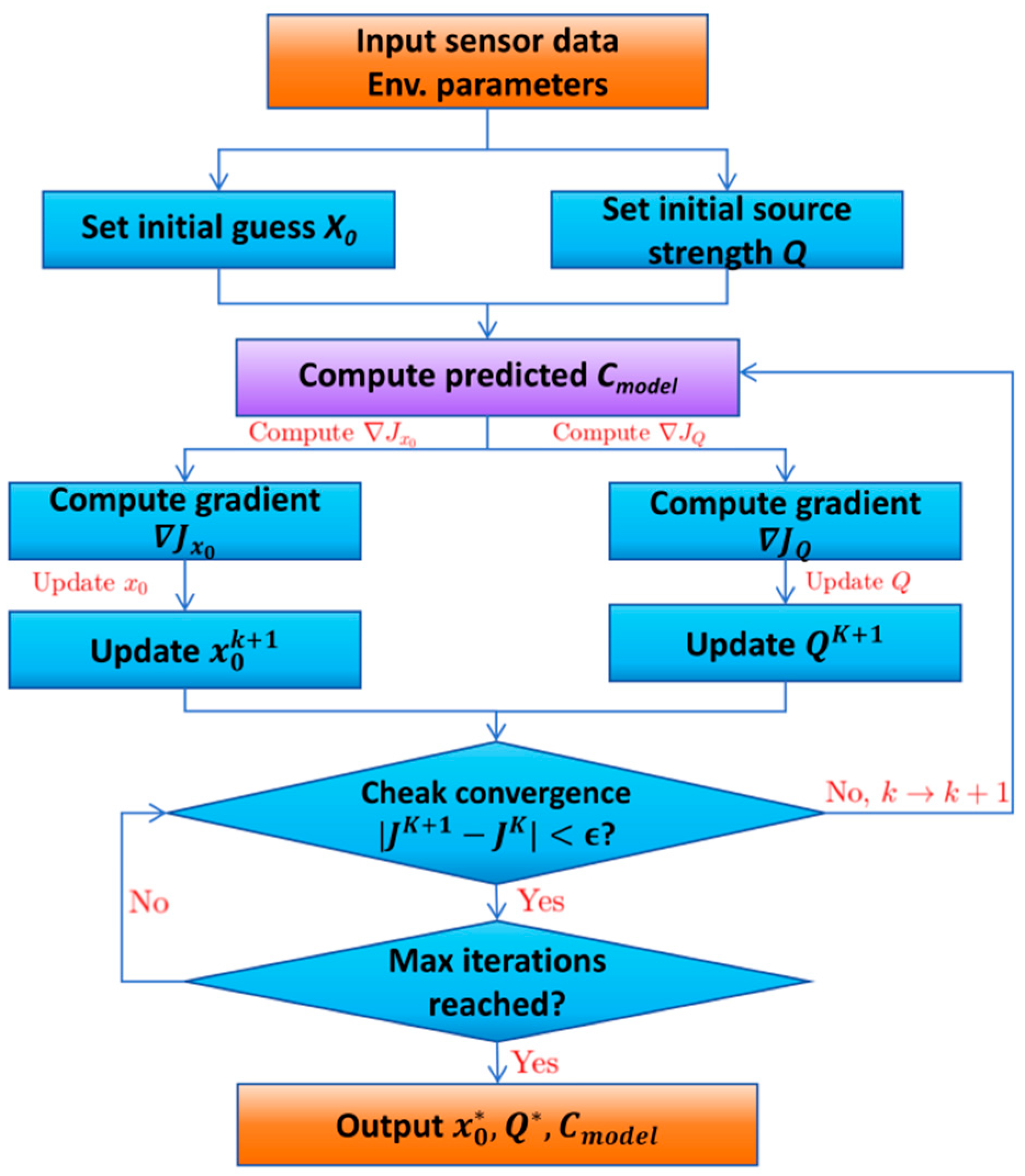
Using the gradient descent numerical optimization algorithm, the direction and step size for adjusting x0 and Q are determined by computing the gradient of the objective error function. During each iteration, the algorithm updates x0 and Q, then recalculates both the predicted concentration Cmodel and the objective error function. The iterative optimization process is illustrated in the flowchart shown in Figure 2.
x 0 k + 1 Q k + 1 = x 0 k Q k α J x 0 k , Q k
Here, α represents the step size (i.e., learning rate) that determines the update speed, and ∇J(x0, Q) denotes the gradient vector of the objective function J, indicating the rate of change of the objective function with respect to x0 and Q:
J x 0 , Q = J x 0 J Q
Gradient computation:
J x 0 = 2 i = 1 n C m o d e l x i , y i , z i ; x 0 , Q C i C m o d e l x 0
J Q = 2 i = 1 n C m o d e l x i , y i , z i ; x 0 , Q C i C m o d e l Q
The optimization process iteratively updates parameters x0 and Q to identify the optimal combination that minimizes the objective function J(x0, Q). The algorithm is considered converged when the target error function satisfies:
J k + 1 J k < ϵ
where ϵ is typically set to 10−6, indicating that the variation in the objective function J(x0,Q) becomes negligible. At convergence, the optimal leakage source location x0∗ and source strength Q∗ are obtained, corresponding to the state where the model-predicted concentrations Cmodel best match the measured concentrations Ci. These converged parameters x0∗ and Q∗ represent the most physically realistic estimates of the leakage source characteristics.

3. Leakage Localization Model Validation

3.1. Numerical Simulation Verification

3.1.1. Simulation Setup

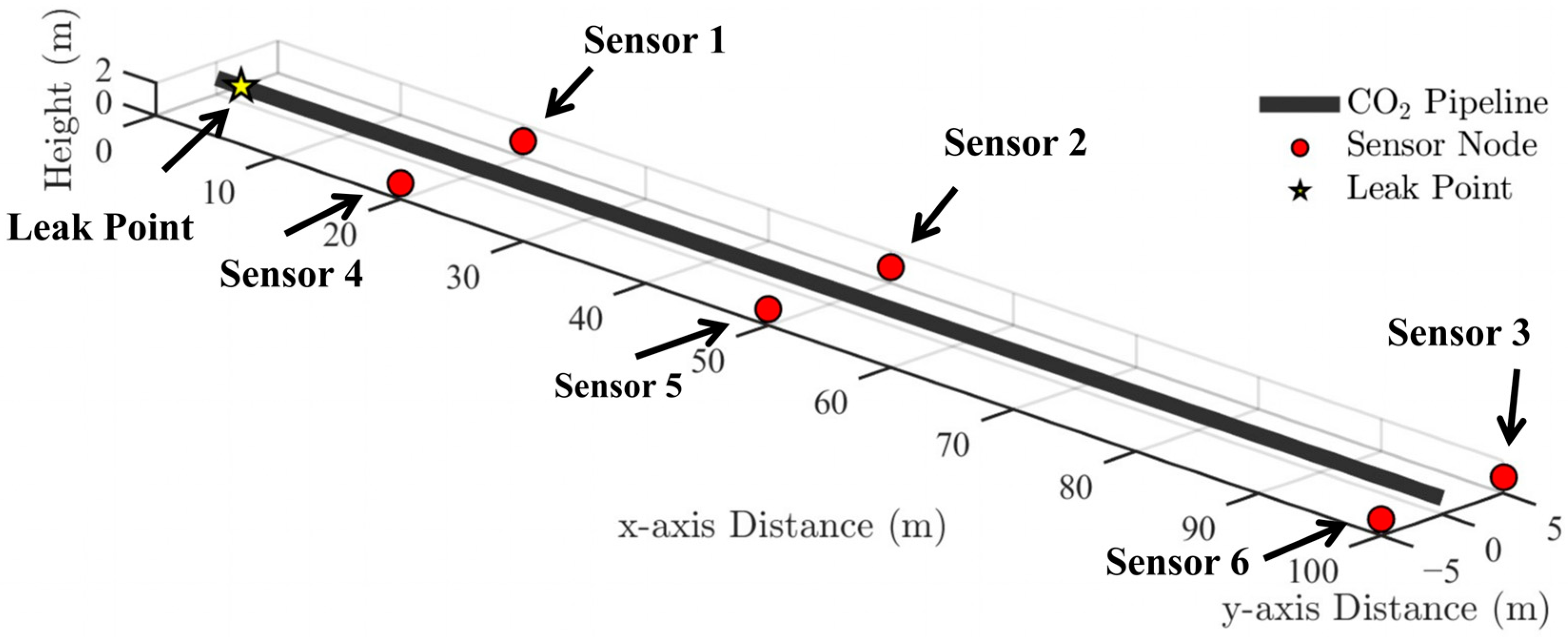
To obtain CO2 concentration data at different positions around the pipeline for validating the proposed model, a three-dimensional gaseous CO2 pipeline leak simulation was established using FLUENT. The pipeline has a length of 100 m, a diameter of 25 mm, and is elevated 1 m above the ground. A three-dimensional Cartesian coordinate system was introduced to provide a spatial reference framework: the pipeline is aligned along the positive x-axis, the y-axis represents the lateral direction, and the z-axis represents height, with z = 0 corresponding to the ground surface. The pipeline centerline is positioned at z = 1 m. The leakage source was positioned 2 m from one end of the pipeline (x = 2 m, y = 0, and z = 1 m), with a controlled mass flow rate of 3.8 kg/s and an ambient wind speed of 1.7 m/s.
Six wireless concentration sensors were arranged along both sides of the pipeline in the downwind direction, with their height aligned to the pipeline centerline (z = 1 m). The sensor positions form a 2 × 3 rectangular grid, and the specific coordinates are provided in Table 1. After initiating the simulated leak, CO2 concentrations at each monitoring point were recorded in real time. These data were subsequently used in conjunction with the proposed inversion model and algorithm to estimate the leak source location and mass flow rate. A schematic illustration of the sensor layout is shown in Figure 3.
Under the simulated experimental conditions, the CO2 concentration data detected simultaneously by each sensor are presented in Table 1. Notably, the sensors were arranged in paired groups on opposite sides of the pipeline, with Sensors 1 and 4 forming one group, Sensors 2 and 5 another group, and Sensors 3 and 6 comprising the third group.

3.1.2. Model Prediction

Fundamental Parameters
The lateral (σy) and vertical (σz) dispersion coefficients in Equation (1) are key parameters for model prediction. Their values are determined based on the Briggs dispersion coefficients (Table 2) and depend on the atmospheric stability [25]. Atmospheric stability is classified according to the Pasquill stability scheme (Table 3), which categorizes stability from A to F based on wind speed and solar radiation, reflecting their influence on turbulent mixing [26]. Specifically, classes A–C represent unstable to slightly unstable conditions, class D indicates neutral conditions, while classes E and F correspond to increasingly stable atmospheric states. For the present study area, the surface wind speed is 1.7 m/s. Considering daytime moderate solar radiation, the atmospheric stability is determined as class B. Subsequently, the lateral and vertical dispersion coefficients corresponding to class B are obtained from Table 2 as functions of the downwind distance x, expressed as σy = 0.16x(1 + 0.0001x)−0.5 and σz = 0.12x, where x denotes the downwind distance from the leakage source to each sensor.
Simulation Results
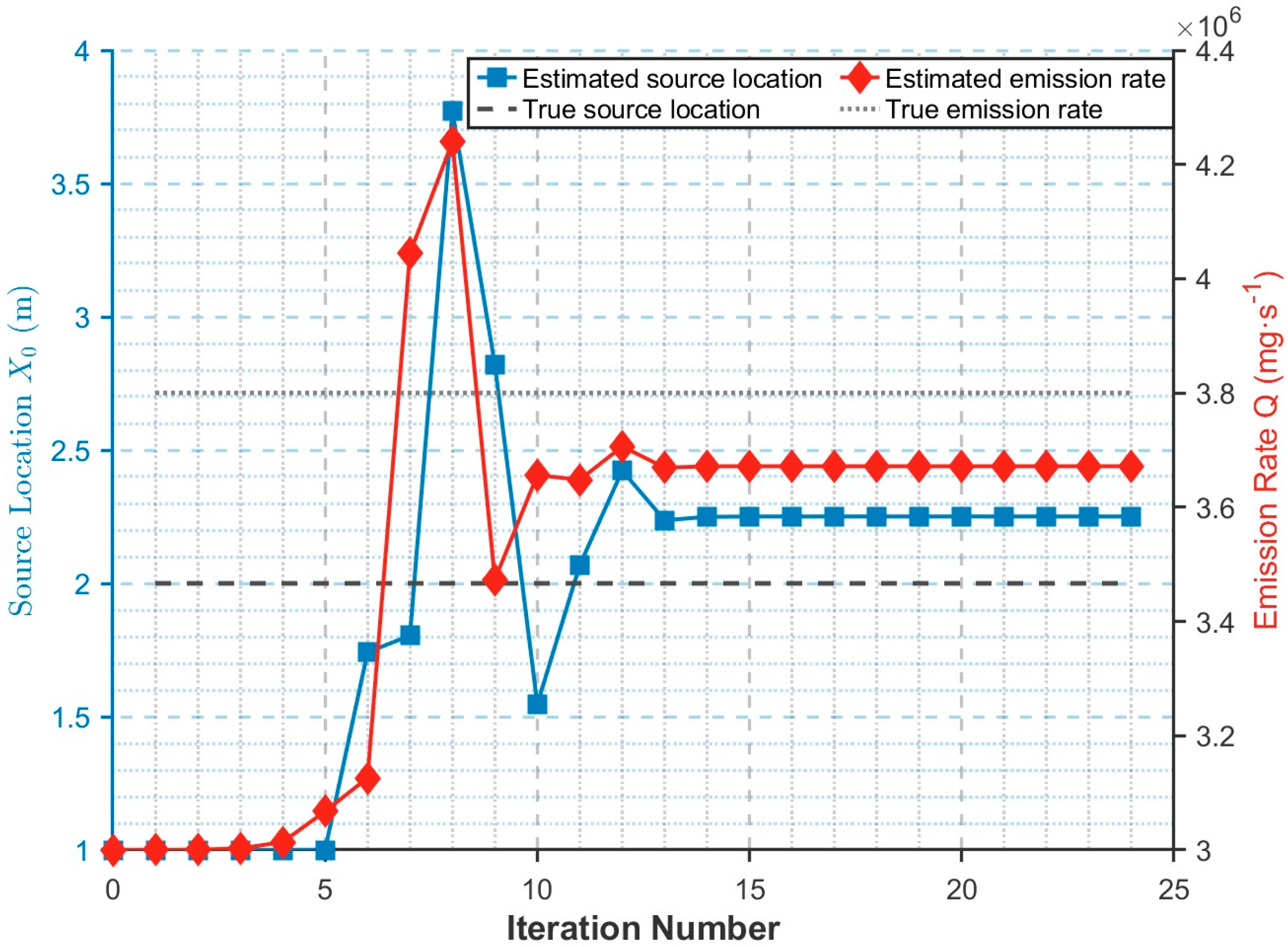
The Gaussian plume dispersion model was employed to calculate the CO2 concentration around the pipeline 30 min after the leakage, aiming to inversely estimate the leakage source location and release rate. A gradient descent numerical optimization algorithm was applied to iteratively solve for the source location x0 and the leakage rate Q, with the iterative process illustrated in Figure 4. The final optimized results were x0 ≈ 2.2507 m and Q ≈ 3671759.2181 mg/s, indicating that the leakage point is located 2.2507 m from one end of the pipeline, with a mass flow rate of approximately 3.67 kg/s.
The optimization involved 24 iterations. During the initial iterations, larger step sizes caused significant adjustments in the estimated values of x0 and Q. As the iteration progressed, the step size gradually decreased, and the predicted source location and release rate converged. After the 24th iteration, both x0 and Q stabilized, with step sizes falling below 10−6, approaching zero, indicating that the optimization process had fully converged.
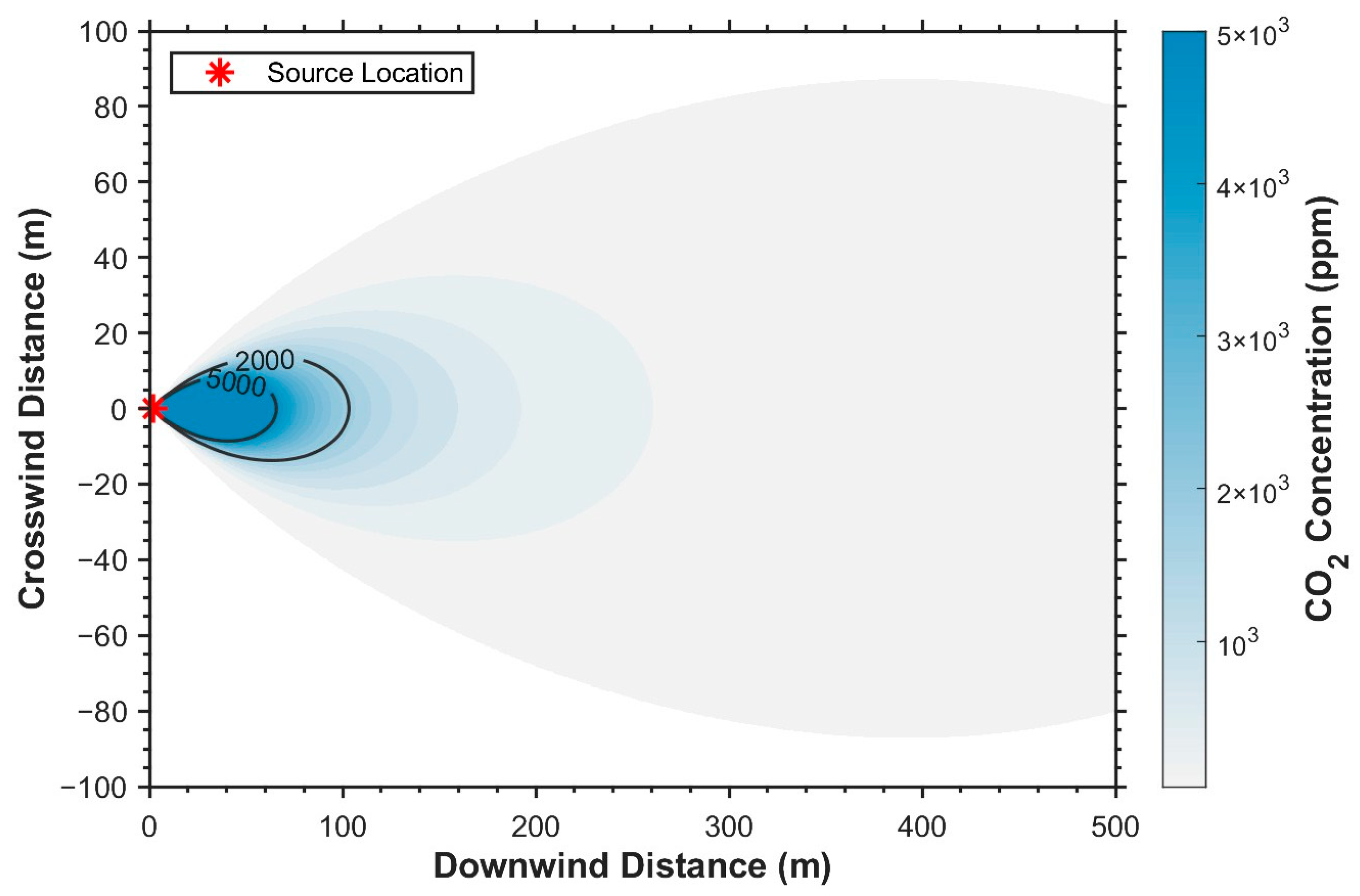
Based on the simulated CO2 concentration data on both sides of the pipeline 30 min after the leakage, the concentration distribution at a height of 1 m is presented in Figure 5. The results show a characteristic fan-shaped dispersion pattern, with contour lines delineating the edges of the plume. Near the leakage point (at x = 2 m), the CO2 concentration reaches its peak, exceeding 1.5 × 10⁵ ppm. Along the downwind direction, the concentration gradually decreases; however, even at the far end of the pipeline (x = 100 m), the concentration remains above 2000 ppm, which may cause discomfort such as shortness of breath and headaches [27]. Influenced by the lateral diffusion coefficient σy, the horizontal spread in the y-direction is relatively limited, although the dispersion range gradually expands with increasing the downwind distance. This figure demonstrates the capability of the Gaussian plume model to predict the concentration distribution of gas leaks under wind conditions, and it captures the characteristic attenuation of gas concentration with distance in realistic leakage scenarios.
Error Analysis
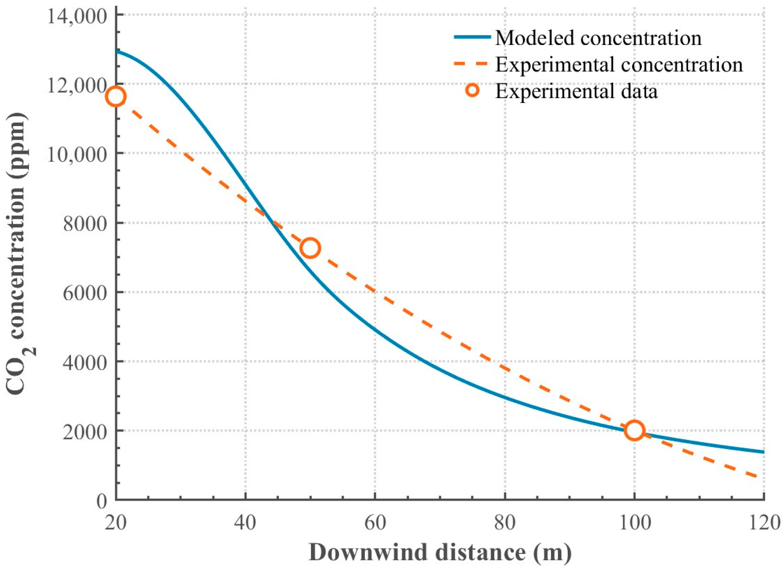
To evaluate the accuracy of the proposed model, the simulation data were compared with the model predictions, as summarized in Table 4. The simulation data represent the averaged CO2 concentrations measured by the sensors on both sides of the pipeline. The comparison indicates that, at three points along one side of the pipeline (x = 20, 50, and 100 m), the concentration errors are approximately 10%, while the leakage source location error is 12.5% and the leakage rate error is 3.5%.
To further assess the predictive performance of the model, a CO2 concentration profile along the pipeline at y = 5 m was generated from the model predictions. Correspondingly, a concentration profile was fitted based on the six simulated sensor measurements, as shown in Figure 6. It can be observed that the predicted values exceed the simulated measurements in the 20–42 m and 100–120 m sections, whereas they are lower than the measurements in the 42–100 m section. Overall, the magnitude of the errors satisfies engineering accuracy requirements, and the predicted concentrations show good agreement with the simulation data, demonstrating the validity of the proposed model.

3.2. Field Experiment Validation

3.2.1. Experimental Platform Setup

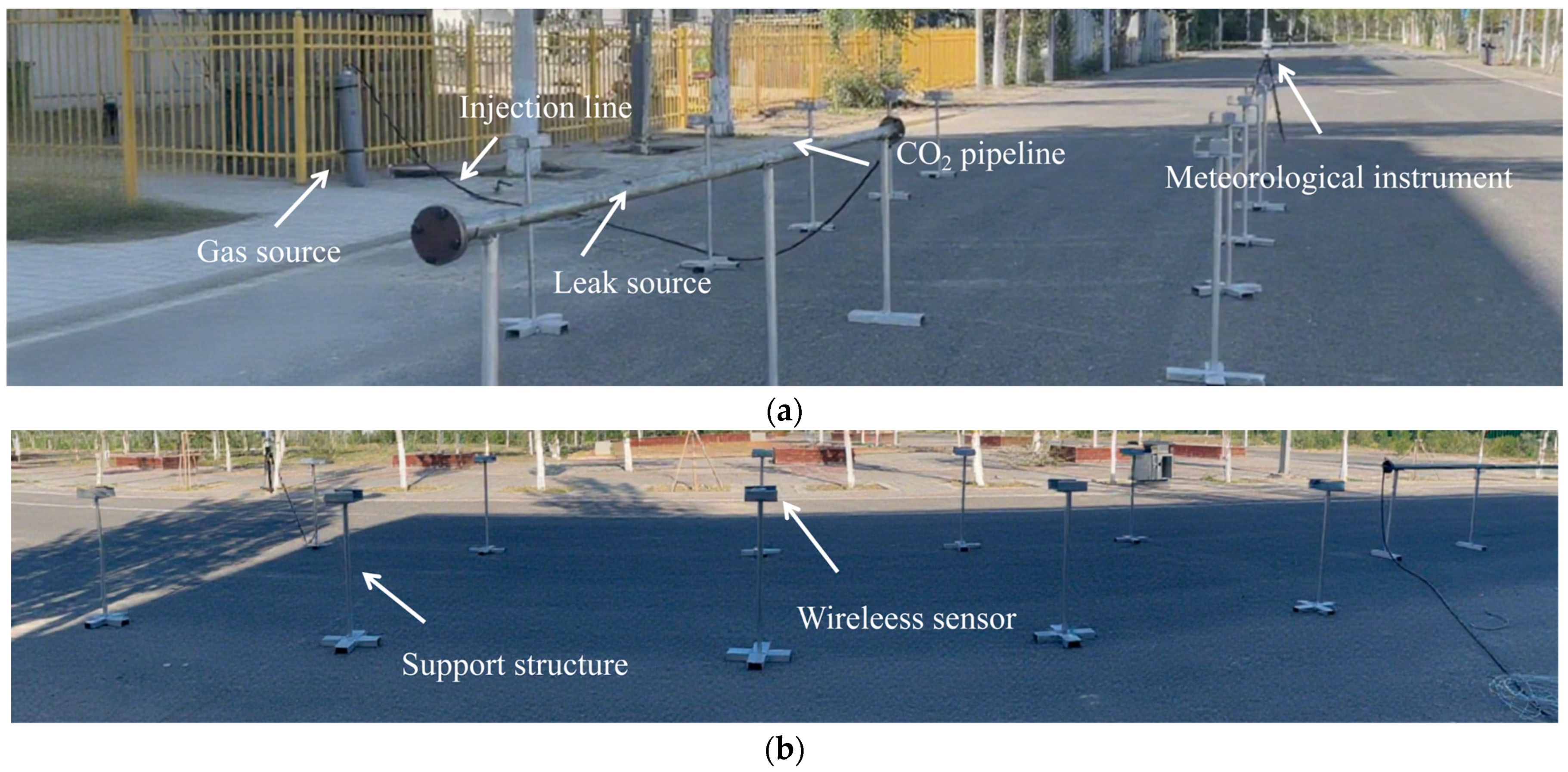
The realistic experimental setup is shown in Figure 7, with (a) presenting the front view and (b) the side view. The field experimental platform constructed in this study consists primarily of a 5 m long, 80 mm diameter high-pressure CO2 pipeline, equipped with a CO2 gas cylinder (rated pressure 5.85 MPa, volume 40 L, and maximum filling capacity approximately 25 kg), along with an injection line and fixing devices, to simulate sudden leakage scenarios that may occur under engineering conditions in a controlled environment. To capture the concentration distribution characteristics at different downwind and lateral positions during leakage, the experimental system was instrumented with ten high-precision CO2 concentration sensors (measurement range: 0–100% and accuracy: ±0.1%). The sensors were deployed in pairs at downwind distances of 5, 10, 15, 20, and 25 m from the leakage source, with a height of 1 m and a lateral offset of 2 m from the pipeline centerline, enabling simultaneous recording of concentration variations on both sides and thereby capturing the lateral dispersion behavior of the gas plume. To simultaneously acquire environmental parameters, the platform was also equipped with a multi-parameter meteorological instrument for real-time monitoring of wind speed, wind direction, temperature, and humidity. All sensors operated at a sampling frequency of 1 Hz and were capable of both wireless data transmission and local storage. The experiment adopted a direct-release method to simulate a pipeline rupture, with a leakage orifice diameter of approximately 10 mm, corresponding to a leakage rate of about 0.21 kg/s. The tests were conducted in an outdoor enclosed safety site with natural wind fields and local turbulence effects, which provided a realistic representation of CO2 dispersion characteristics during actual leakage accidents. The initial experimental conditions are summarized in Table 5.

3.2.2. Experimental Results

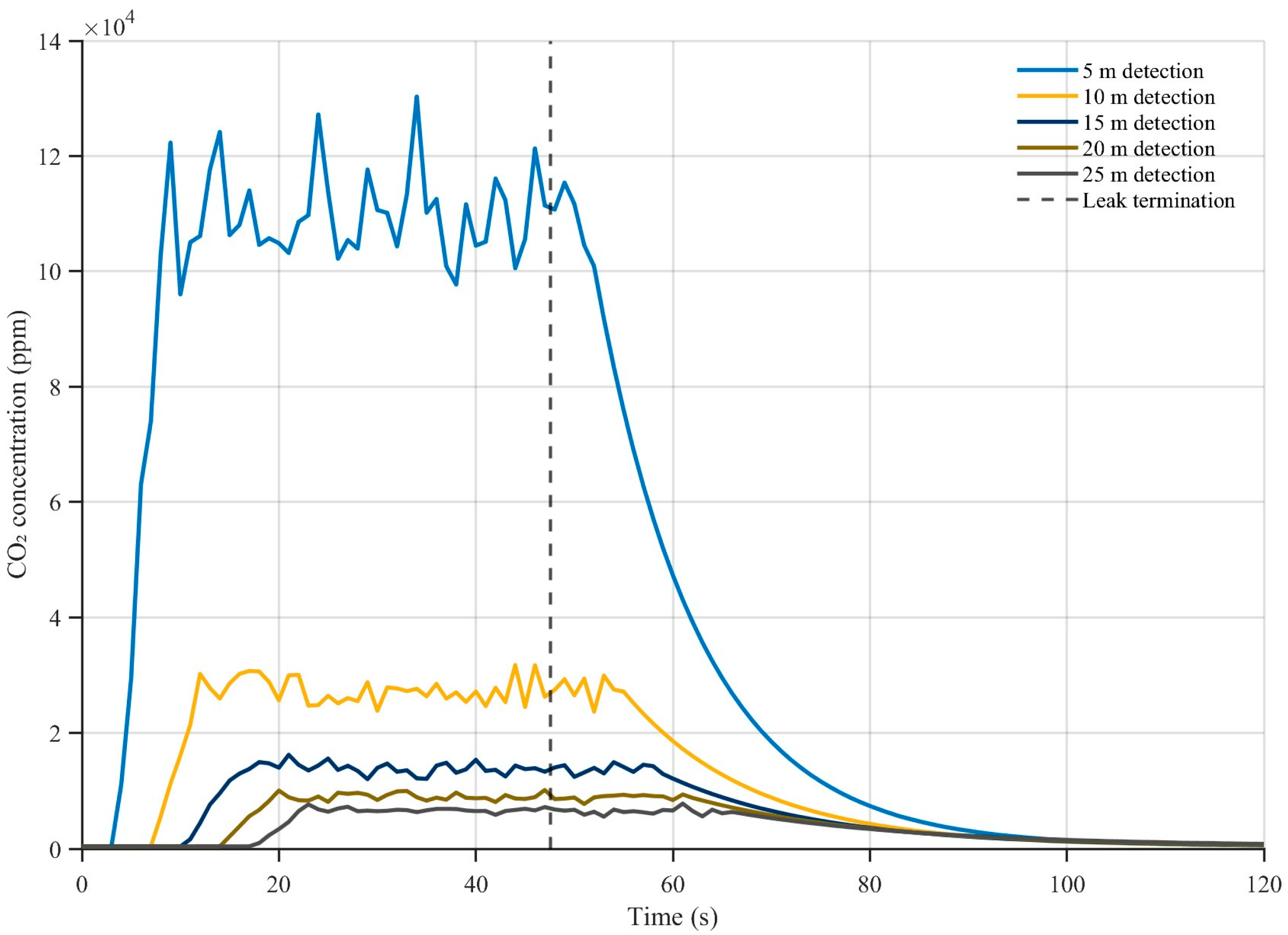
During the field test, all ten CO2 concentration sensors continuously recorded the temporal evolution of the gas concentration following the leakage. The overall pattern exhibited a rapid increase to a peak followed by a gradual decay, as illustrated in Figure 8 for different downwind positions.
The sensor located 5 m from the leak responded first, reaching a peak concentration of 130,296.7 ppm at 21.8 s. With increasing the downwind distance, the peak occurrence was progressively delayed to 10 m (27.4 s), 15 m (32.6 s), 20 m (36.8 s), and 25 m (42.2 s), while the corresponding peak concentration decreased to 7801.0 ppm, exhibiting an exponential decay consistent with atmospheric dilution and dispersion characteristics. After the leakage ceased at 47.6 s, the CO2 concentrations at all monitoring points rapidly declined and returned to the ambient level (~400 ppm) at approximately 60 s.
Overall, the observed spatial attenuation and temporal delay along the downwind direction were in agreement with the theoretical predictions, confirming the rationality of sensor deployment and the effectiveness of the experimental design. These results provide a reliable basis for validating the predictive model.
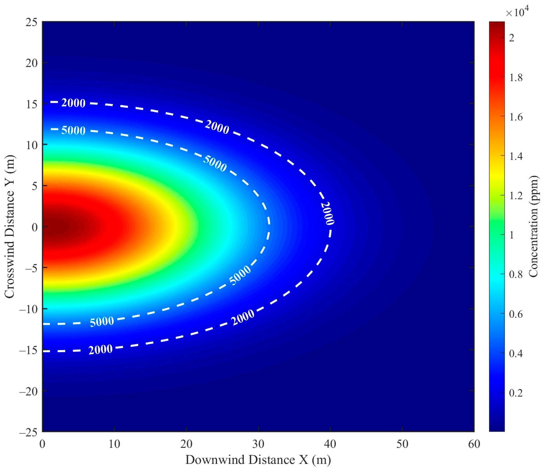
Figure 9 illustrates the CO2 concentration distribution following the pipeline leak, along with the associated potential hazard zones. The highest concentrations were observed near the leakage source, with the gas exhibiting a fan-shaped dispersion pattern along the downwind direction, indicating pronounced directional spread. The 5000 ppm iso-concentration contour was located approximately 27–31 m from the leak, representing a level sufficient to induce acute asphyxiation and thus serving as a critical safety boundary. The 2000 ppm contour extended further downwind, approximately 38–42 m from the source; although lower, prolonged exposure at this level may still cause adverse physiological effects [28,29]. Overall, the CO2 concentration decreased rapidly with distance, yet the presence of high-concentration zones poses a significant operational hazard. Therefore, personnel should evacuate promptly and ensure adequate ventilation to mitigate health risks in the event of a leak.

3.2.3. Model Validation

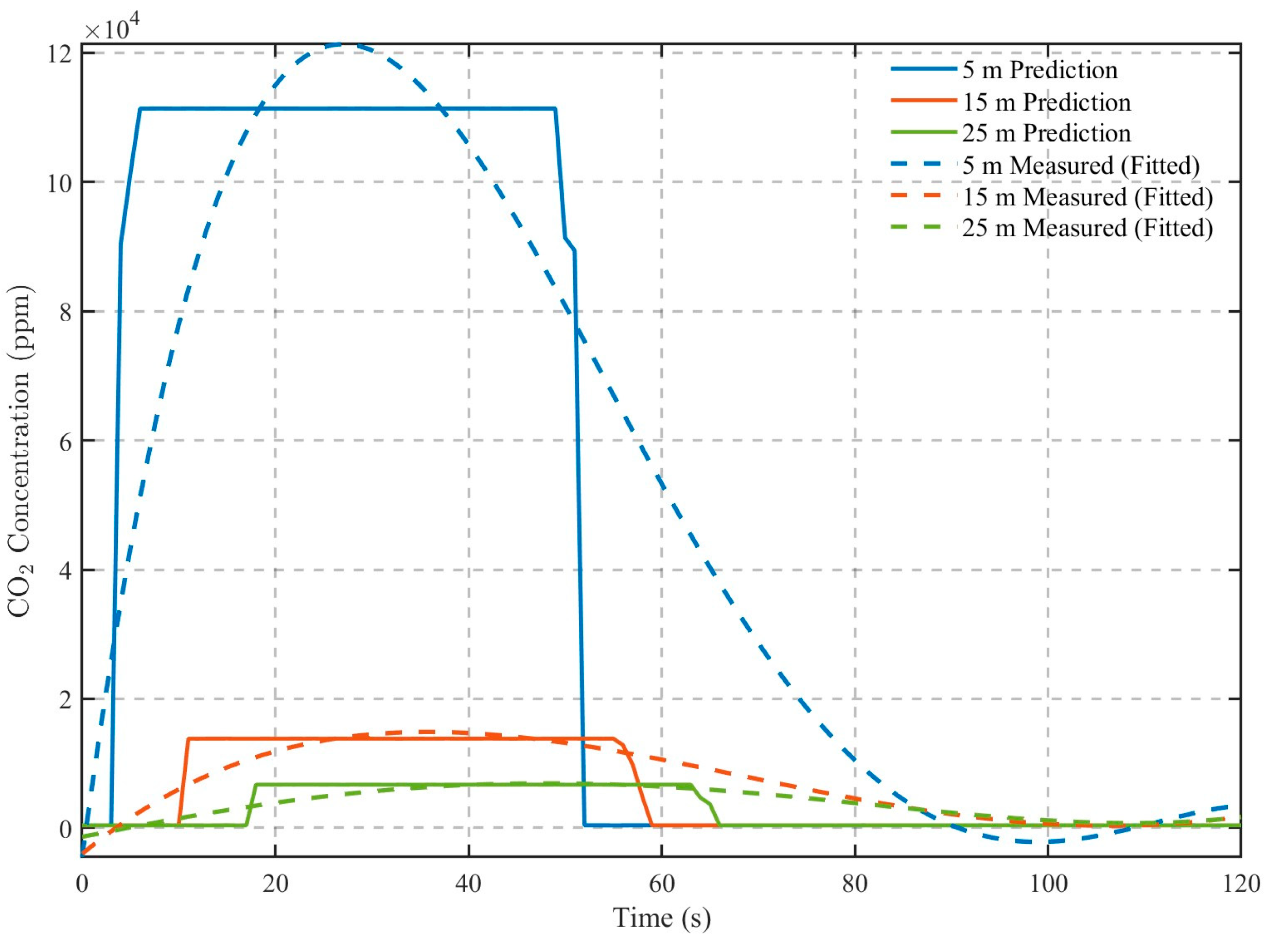
To evaluate the practical applicability of the proposed Gaussian plume inversion model, three representative monitoring points were selected at near-field (5 m), mid-field (15 m), and far-field (25 m) locations, corresponding to high-concentration, transition, and dilution zones, respectively, to comprehensively capture the spatial evolution of CO2 concentrations during the leakage process. Temporal comparisons at the representative points are shown in Figure 10. The model results indicate that, in terms of concentration distribution, the near-field (5 m) predicted value deviates from the measured value by approximately 8.96%. Since the model does not account for complex factors such as terrain, topography, or obstacles, the predicted peak concentration occurs earlier, reaching its maximum at 6 s, whereas the measured peak occurs roughly 20.9 s later, at approximately 26.9 s. This suggests that the model can capture the temporal evolution of concentration changes, providing valuable information for risk assessment and emergency response, thus demonstrating its potential practical value for safety applications.
At the mid-field (15 m) and far-field (25 m) points, the deviations between predicted and measured concentrations are approximately 7.56% and 2.9%, respectively, with peak occurrences preceding the measured peaks by 25.8 s and 30.1 s. The decreasing discrepancy with increasing distance is primarily attributed to enhanced turbulent dispersion of CO2, which reduces the influence of local disturbances on the overall concentration distribution, thereby narrowing the gap between model predictions and measurements.
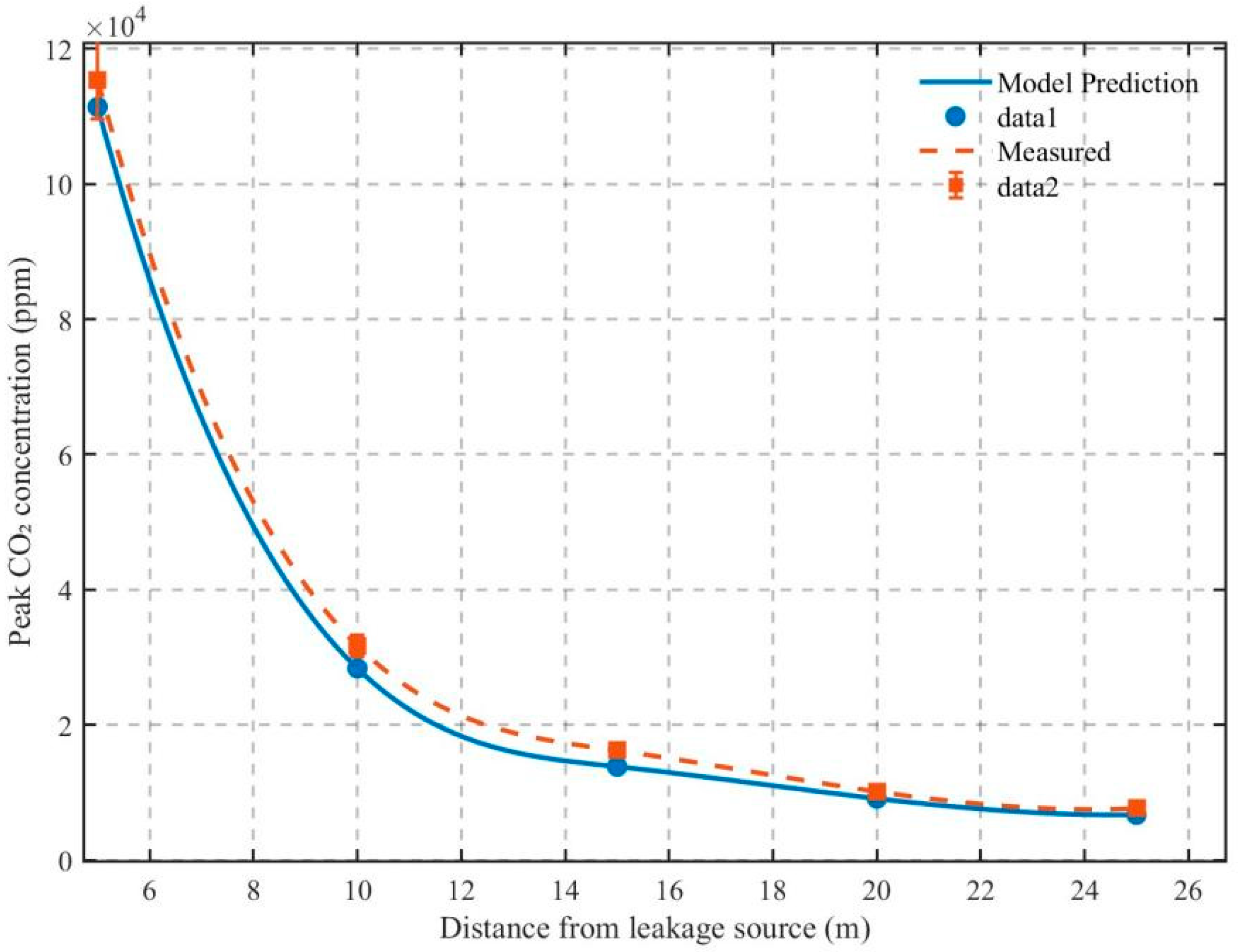
The peak concentration serves as a critical indicator for assessing the safety risks associated with gas leakage, as both its magnitude and occurrence time directly influence the severity of the incident and the efficiency of emergency response. Therefore, validating the predictive capability of the model is essential. As shown in Figure 11, the predicted concentration profiles closely match the measured data, with errors ranging from 3.5% to 14.7%, indicating that the model not only accurately captures the spatial attenuation characteristics of the gas but also demonstrates high predictive accuracy.
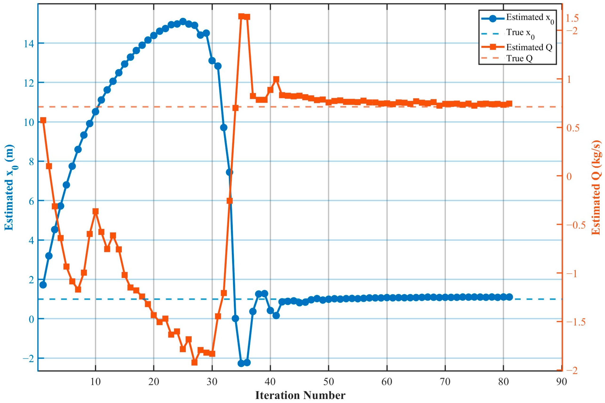
Figure 12 illustrates the convergence process of the inverse calculation for the leak source location and emission rate. The results indicate that the final converged value of the leak location x0 exhibits a relative error of approximately 16.9% compared to the true leak position (1 m), while the inversely estimated leak rate Q differs from the actual value of 0.21 kg/s by about 13.9%. Overall, although some deviation exists between the inverse results and the true values, the method is capable of determining the leak source location and emission rate with reasonable accuracy within a short period, providing a rapid approach for tracing unexpected gas leak incidents.

4. Model Adaptability Analysis

4.1. Effect of Sensor Number on Model Localization Accuracy

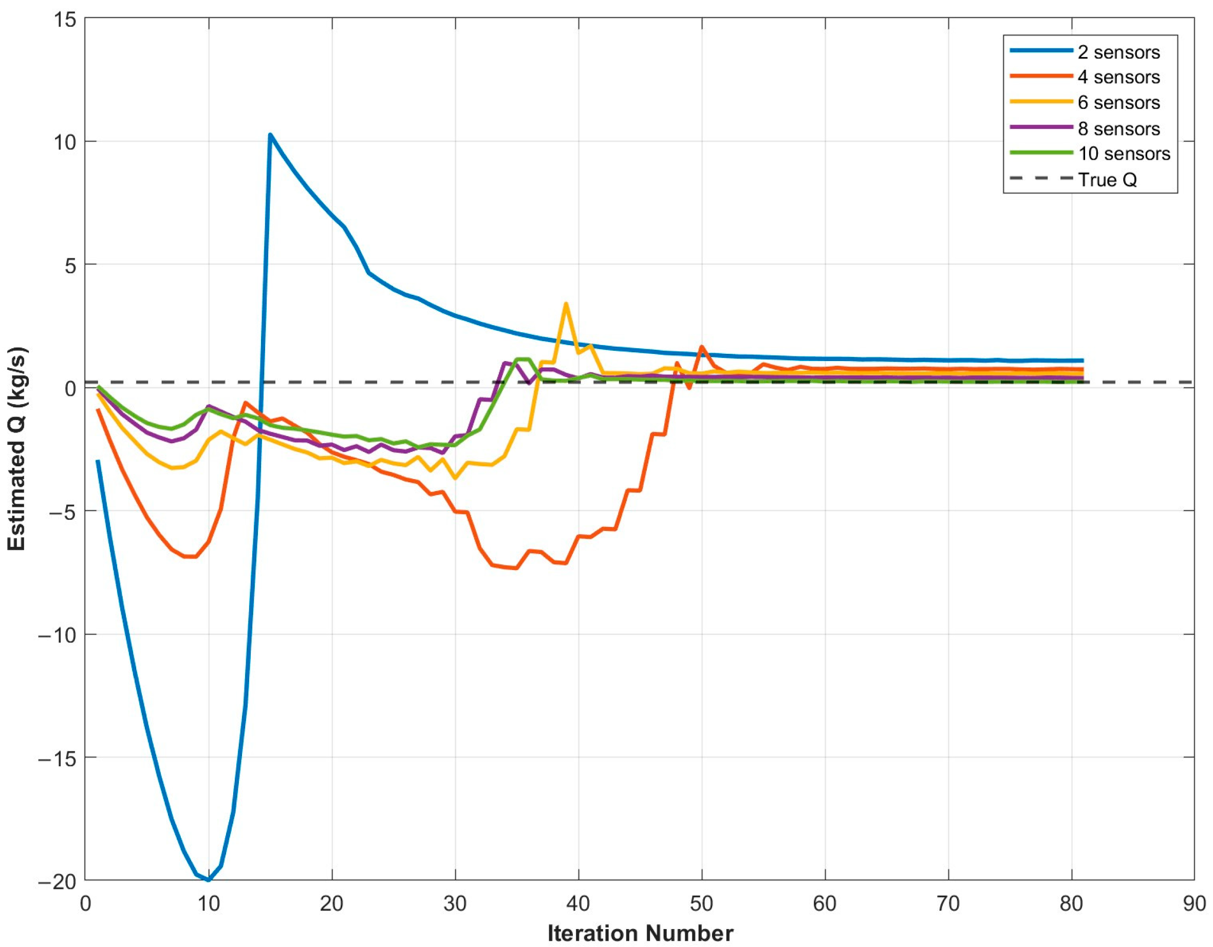
The number and deployment layout of sensors directly determine the data constraints during the model inversion process, thereby significantly affecting the accuracy of leak source localization and emission rate estimation. To systematically investigate this effect, this study configured 2, 4, 6, 8, and 10 sensors for data acquisition and compared the inversion results of the leak source location and emission rate under different sensor numbers.
Figure 13 and Figure 14 illustrate the iterative inversion processes of the leak emission rate and source location, respectively, for varying sensor numbers. It can be observed that, as the number of sensors increases, the final inversion results for both emission rate and source location progressively approach the true values, demonstrating a clear improvement in convergence performance.
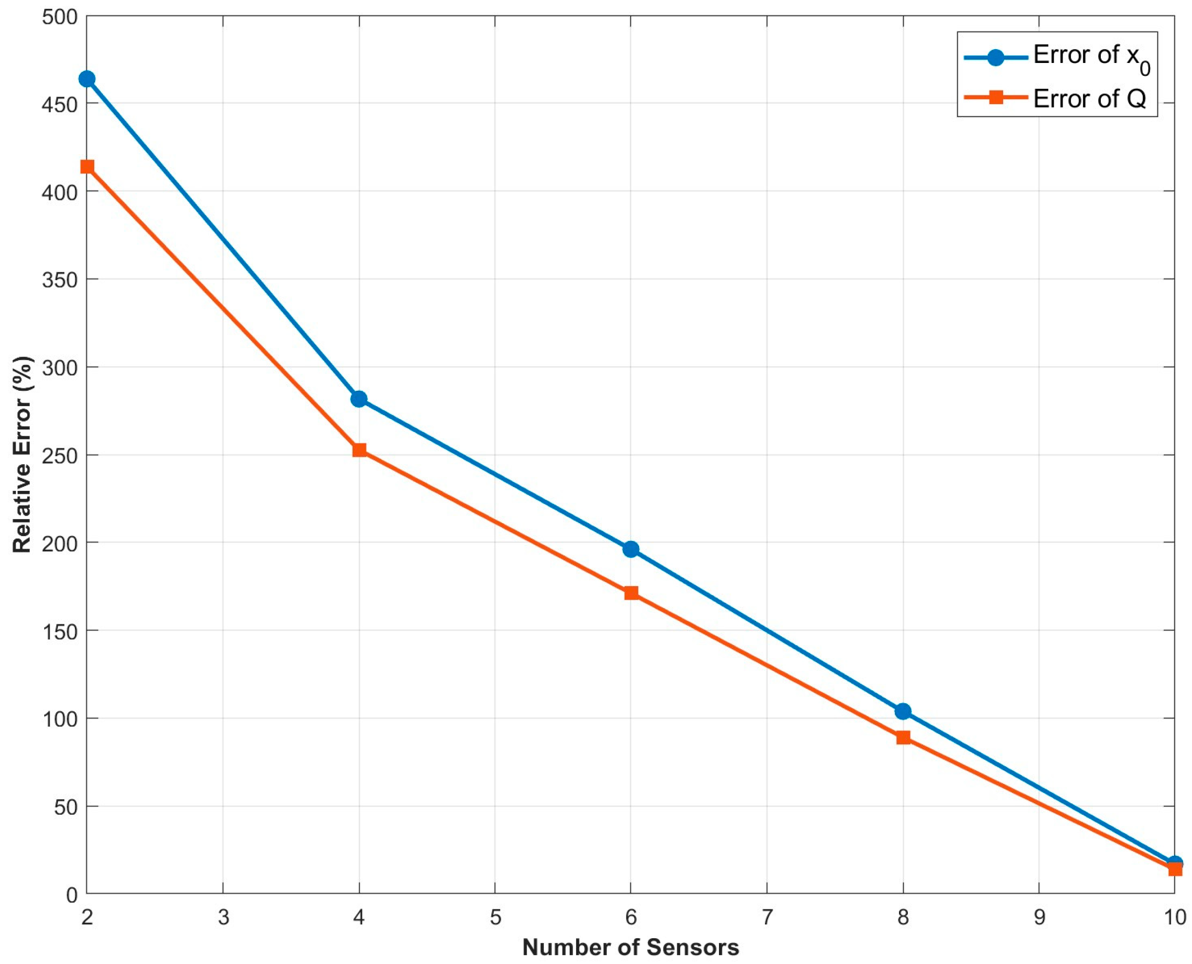
Figure 15 presents a comparison of model prediction errors under different numbers of sensors. It can be observed that the inversion errors decrease significantly as the number of sensors increases. With only two sensors, the prediction errors for leak location and leak rate are as high as 463.8% and 413.8%, respectively, rendering the inversion results practically unusable for engineering applications. When the number of sensors is increased to six, the errors decrease markedly to 196.1% and 171.1%. Further increasing the sensor count to ten reduces the errors to 16.9% and 13.9%, meeting the accuracy requirements for practical engineering applications.
The above results indicate that increasing the number of sensors can significantly enhance the inversion accuracy of the model. When the sensor count is insufficient, spatial constraints are limited, which may lead to deviations or convergence to local optima. In contrast, an adequate number of sensors provides multi-point observations that fully support the inversion process, thereby improving prediction accuracy. Therefore, in practical applications, sensor deployment should be optimized by considering factors such as terrain, wind conditions, and cost.

4.2. Influence of Leak Source Characteristics on Model Applicability

Depending on the release characteristics of the leak source and the study objective, Gaussian dispersion models typically take three common forms: the Gaussian plume model, the Gaussian puff model, and the Gaussian sphere model [30]. The Gaussian plume model is suitable for continuously releasing sources along the wind direction, capable of forming a stable plume and predicting long-term concentration distributions [31]. The Gaussian puff model is appropriate for instantaneous point-source releases, where the leaked substance disperses as localized high-concentration “puffs” and its concentration decays over time [32]. The Gaussian sphere model is mainly used for theoretical analyses or under homogeneous environments, where the concentration exhibits spherical symmetry [33]. As summarized in Table 6, different models correspond to distinct source types and concentration distribution characteristics.
In this study, the Gaussian plume model is employed, which is most suitable for continuous source leak scenarios. For point-source or instantaneous releases, the Gaussian plume model has limitations in predicting instantaneous concentration gradients and local peak values. Similarly, for theoretical homogeneous three-dimensional dispersion scenarios, the plume assumption is not fully applicable. As indicated in Table 6, the applicable range of different Gaussian models varies in engineering practice. Therefore, in practical applications, the selection of an appropriate observation scheme should be based on the type of leak source, so as to fully leverage the advantages of the Gaussian plume model in monitoring continuous leaks.

4.3. Influence of Wind Speed on Model Prediction Performance

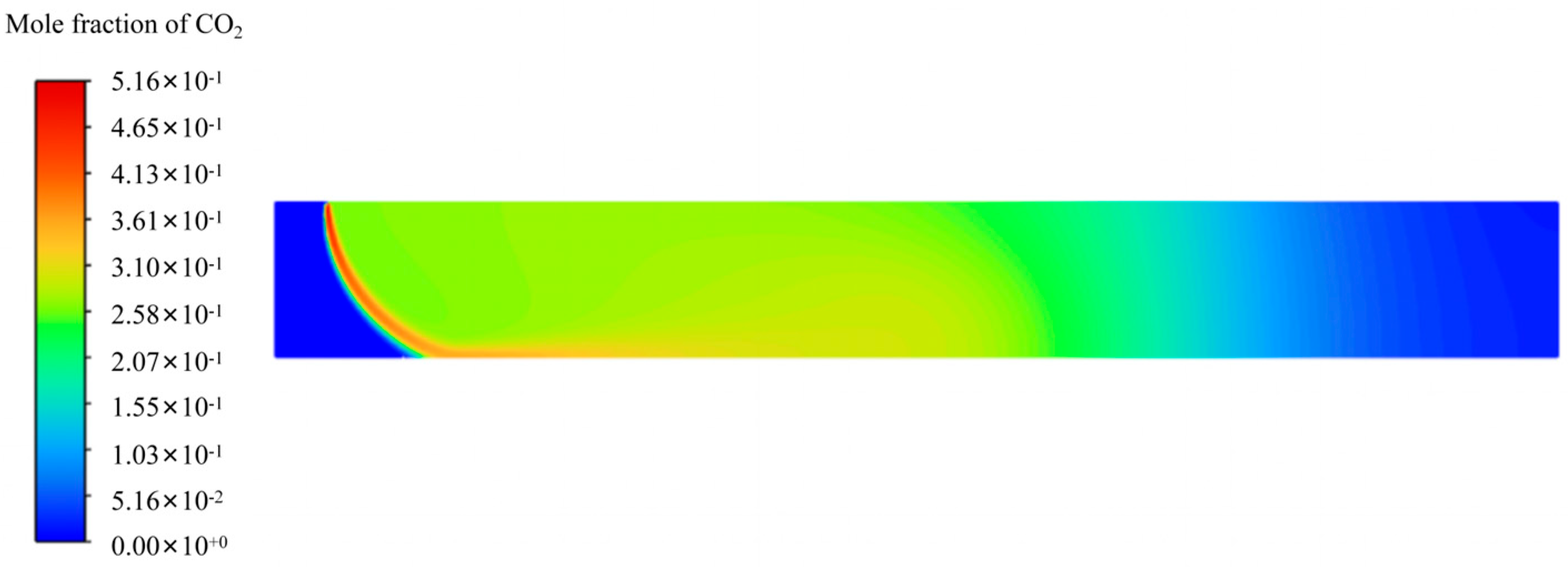
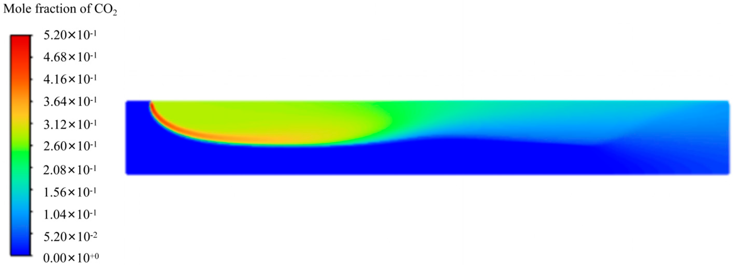
To investigate the effect of wind speed on the prediction performance of the Gaussian plume inversion model, FLUENT simulations were conducted to track the evolution of the CO2 concentration under different wind conditions. As shown in Figure 16, under low wind speed (e.g., 1 m/s), air convection is weak, causing the leaked gas to remain in the near-source region for an extended period and delaying the time required for the concentrations to reach a steady state. In contrast, at higher wind speed (e.g., 5 m/s), as illustrated in Figure 17, the gas is rapidly transported, leading to fast downwind dispersion and a quicker stabilization of the system. These results indicate that wind speed significantly affects the dispersion rate and concentration distribution of the leaked gas, thereby influencing the accuracy of source strength and location predictions. Therefore, wind speed must be considered in inversion analyses to ensure reliable results.

5. Engineering Application

In practical engineering, CO2 pipeline leak monitoring requires consideration of high-risk locations, sensor deployment, and the coordinated operation of wireless sensor networks. Vulnerable points such as elbows, flanges, and welds are prone to leaks and should be designated as key monitoring locations [34]. Strategic placement of sensors in downwind areas or low-lying terrains can effectively capture gas dispersion patterns, while sensors along low-risk straight sections may be spaced more widely to balance monitoring accuracy and cost efficiency. Data collected by the sensors are transmitted in real time to the processing center via the WSN. Low-power communication protocols, such as LoRa or ZigBee, can achieve coverage over tens to hundreds of kilometers of pipeline using multi-hop mechanisms, and 4G or satellite links may be supplemented when necessary to ensure communication reliability [35]. It should be emphasized that a standalone WSN can provide real-time leak detection but is insufficient for direct leak source inversion and quantitative risk assessment. The integration of WSNs with the Gaussian plume model enables rapid source localization and leak quantification. Compared to technologies such as fiber-optic sensing or infrared remote sensing, this approach offers flexible deployment and lower cost, demonstrating strong potential for engineering application [36].
The long-term stable operation of the system also depends on power supply and equipment durability. Short-term tests may rely on battery power, whereas long-term operation typically employs a combination of solar panels and rechargeable batteries, with wired power available at critical stations. Sensors must possess waterproof, dustproof, and corrosion-resistant characteristics and maintain stable performance over a wide temperature range to adapt to the uncertainties of field environments. Overall, the system can be extended for full-line monitoring of long-distance pipelines while effectively balancing safety and cost, providing robust technical support for emergency response and risk management.

6. Conclusions

(1)
This study addresses the problem of CO2 pipeline leak detection and localization by integrating a wireless sensor network with the Gaussian plume model, thereby establishing a comprehensive CO2 leak detection and localization framework. Comparisons between model predictions and simulated experimental measurements indicate a leak location error of approximately 12.5% and a leak rate error of approximately 3.5%, meeting engineering accuracy requirements. The model enables rapid localization of the leak point and prediction of the CO2 concentration distribution along the pipeline, providing technical support for safe pipeline operation.
(2)
Field experiments further validated the applicability of the model. The predicted concentration profiles closely match the measured data, with errors controlled within 3.5–14.7%, accurately capturing the dispersion patterns and concentration variations at different distances. Moreover, the number and spatial arrangement of sensors significantly affect the inversion accuracy; optimized sensor deployment can enhance leak localization precision and source strength estimation reliability. The combination of WSN and the Gaussian plume model demonstrates clear advantages over standalone WSNs in rapid leak localization, source strength estimation, and risk prediction.
(3)
The model’s performance under complex meteorological conditions, multi-source leaks, and optimal WSN node placement requires further investigation. Future work will focus on optimizing sensor layout and incorporating multi-source data along with environmental parameter corrections to enhance the model’s robustness and accuracy in real-world complex scenarios, providing more comprehensive and reliable technical support for CO2 pipeline leak detection.

Author Contributions

Conceptualization, X.L. and F.L.; methodology, F.L.; software, F.L., J.C., Z.W., D.W. and Y.R.; validation, X.L., F.L. and Z.W.; formal analysis, F.L.; investigation, X.L. and J.C.; resources, X.L., D.W. and Y.R.; data curation, X.L., F.L. and J.C.; writing—original draft preparation, X.L., F.L. and J.C.; writing—review and editing, X.L., F.L. and J.C.; visualization, X.L., F.L. and Z.W.; supervision, F.L.; project administration, X.L.; funding acquisition, X.L. All authors have read and agreed to the published version of the manuscript.

Funding

Supported by the National Natural Science Foundation of China for Regional Fund (52562047); Natural Science Foundation of Xinjiang Uygur Autonomous Region (2023D01A19); Xinjiang Uygur Autonomous Region “Tianchi talents” introduction plan project (TCYC12); Xinjiang Tianshan Innovation Team for Research and Application of High-Efficiency Oil and Gas Pipeline Transportation Technology (2022TSYCTD0002); Xinjiang Uygur Region “One Case, One Policy” Strategic Talent Introduction Project (XQZX20240054).

Data Availability Statement

The original contributions presented in this study are included in the article. Further inquiries can be directed to the corresponding author.

Conflicts of Interest

The authors declare no conflicts of interest.

References

  1. Lu, H.; Guo, L.; Azimi, M.; Huang, K. Oil and Gas 4.0 era: A systematic review and outlook. Comput. Ind. 2019, 111, 68–90. [Google Scholar] [CrossRef]
  2. Ebi, K.L.; Boyer, C.; Ogden, N.; Paz, S.; Berry, P.; Campbell-Lendrum, D.; Hess, J.J.; Woodward, A. Burning embers: Synthesis of the health risks of climate change. Environ. Res. Lett. 2021, 16, 044042. [Google Scholar] [CrossRef]
  3. Rockström, J.; Gaffney, O.; Rogelj, J.; Meinshausen, M.; Nakicenovic, N. A roadmap for rapid decarbonization. Science 2017, 376, 870–872. [Google Scholar] [CrossRef]
  4. Khan, M.D.; Khushnood, M.; Ali, M.; Imran, H. A techno-economic assessment of CO2 pipeline transportation in Asia: Challenges and future prospects. Energy Rep. 2022, 8, 4680–4692. [Google Scholar] [CrossRef]
  5. Cao, Z.; Hu, Y.; Chen, L.; Yan, X.; Yu, S.; Yu, J. Experimental study of leakage characteristics and risk prediction of N2-containing dense-phase CO2 pipelines in real transportation conditions. Process Saf. Environ. Prot. 2024, 187, 1112–1125. [Google Scholar] [CrossRef]
  6. Hu, Q.; Zhang, H.; Zhao, X.; Meng, L.; Li, Y.; Zhang, L.; Zhu, J.; Wang, W. Carbon dioxide pipeline leakage risk assessment based on pipeline failure probability correction and CO2 concentration dispersion distance prediction. J. Pipeline Sci. Eng. 2025, 5, 100293. [Google Scholar] [CrossRef]
  7. Jacobson, T.A.; Kler, J.S.; Hernke, M.T.; Braun, R.K.; Meyer, K.C.; Funk, W.E. Direct human health risks of increased atmospheric carbon dioxide. Nat. Sustain. 2019, 2, 691–701. [Google Scholar] [CrossRef]
  8. Chen, L.; Hu, Y.; Liu, Z.; Yan, X.; Yu, S.; Ding, J.; Liu, P. Experimental research on the fracture and arrest process of supercritical CO2 pipelines. Int. J. Press. Vessels Pip. 2024, 208, 104000. [Google Scholar] [CrossRef]
  9. Clarion Ledger. Hundreds Evacuated, Dozens Hospitalized After Gas Pipe Rupture in Mississippi. Clarion Ledger, 23 February 2020. Available online: https://time.com/5789425/pipe-rupture-mississipi/ (accessed on 15 September 2025).
  10. Lakhani, N. ‘Wake-up call’: Pipeline Leak Exposes Carbon Capture Safety Gaps, Advocates Say. The Guardian, 19 April 2024. Available online: https://www.theguardian.com/us-news/2024/apr/19/exxon-pipeline-leak-carbon-capture-safety-gaps (accessed on 8 May 2025).
  11. Bonne, J.-L.; Donnat, L.; Albora, G.; Burgalat, J.; Chauvin, N.; Combaz, D.; Cousin, J.; Decarpenterie, T.; Duclaux, O.; Dumelié, N. A measurement system for CO2 and CH4 emissions and an evaluation of Gaussian-plume atmospheric inversion approaches. Atmos. Meas. Tech. 2024, 17, 4471–4490. [Google Scholar] [CrossRef]
  12. Zhao, J.; Li, J.; Bai, Y. Research on leakage detection technology of natural gas pipeline based on modified Gaussian plume model and Markov chain Monte Carlo method. Process Saf. Environ. Prot. 2023, 174, 138–150. [Google Scholar] [CrossRef]
  13. Newman, T.; Nemeth, C.; Jones, M.; Jonathan, P. Probabilistic inversion modeling of gas emissions: A gradient-based MCMC estimation of Gaussian plume parameters. Atmos. Environ. 2024, 318, 120217. [Google Scholar] [CrossRef]
  14. Sun, C.; Yan, Y.; Zhang, W.; Shao, D. Measurement of CO2 leakage from pipelines under CCS conditions: Methodology for continuous quantification. Int. J. Greenh. Gas Control 2024, 237, 115164. [Google Scholar] [CrossRef]
  15. Aminaho, N.S.; Aminaho, E.N. Artificial Intelligence Based Solutions for CO2 Pipeline Monitoring: A Review. SSRN Working Paper 2025. Available online: https://papers.ssrn.com/sol3/papers.cfm?abstract_id=5265609 (accessed on 15 September 2025).
  16. Marchi, A.; Cavalagli, N.; Ubertini, F. Experimental investigations of distributed fiber optic sensors for pipeline monitoring. Sensors 2023, 23, 6205. [Google Scholar] [CrossRef]
  17. Gong, Y.; Liu, Z.; Li, W.; Bao, C.; He, Z.; Jian, Y.; Wang, X.; Huang, H.; Song, X. A review on gas pipeline leak detection: Acoustic-based methods and applications. Information 2025, 16, 731. [Google Scholar] [CrossRef]
  18. Wang, X.; Xu, M.; Yang, Y.; Jiang, Z. Heterogeneous data fusion model for gas leakage detection. J. Loss Prev. Process Ind. 2025, 98, 105767. [Google Scholar] [CrossRef]
  19. Kolosov, A.; Large, S.; Inbar, E. Distributed fiber-optic sensing (DAS/DTS) for oil and gas pipeline monitoring: A review. J. Pet. Sci. Eng. 2022, 210, 110072. [Google Scholar] [CrossRef]
  20. Kang, Z.; Qian, X.; Li, Y.; Hou, L.; Huang, Z.; Duanmu, W.; Yuan, M. Feature extraction of natural gas leakage for an intelligent warning model: A data-driven analysis and modeling. Process Saf. Environ. Prot. Trans. Inst. Chem. Eng. Part B 2023, 109, 104823. [Google Scholar] [CrossRef]
  21. Nguyen, H.A.D.; Le, T.H.; Azzi, M.; Ha, Q.P. Monitoring and estimation of urban emissions with low-cost sensor networks and deep learning. Ecol. Inform. 2024, 82, 102750. [Google Scholar] [CrossRef]
  22. Zhou, Z.; Yang, Y.; Shi, Y.; Wang, Y.; Wu, W.; Qu, G. Observing CO2 emissions from global key coal-fired power plants based on Orbiting carbon Observatory-3 satellite and improved Gaussian plume model. J. Clean. Prod. 2025, 518, 145245. [Google Scholar] [CrossRef]
  23. Zhu, Z.; Chen, B.; Zhao, Y.; Ji, Y. Multi-sensing paradigm based urban air quality monitoring and hazardous gas source analyzing: A review. J. Saf. Sci. Resil. 2021, 2, 131–145. [Google Scholar] [CrossRef]
  24. Cheng, W.; Liu, X. An adaptive Gaussian dispersion model for air pollution simulation with complex terrain constraints. Atmos. Environ. 2021, 254, 118358. [Google Scholar] [CrossRef]
  25. Ražnjević, A.; van Heerwaarden, C.; Krol, M. Evaluation of two common source estimation measurement techniques: Methane plume dispersion using real-time sensors. Atmos. Meas. Tech. 2022, 15, 3611–3623. [Google Scholar] [CrossRef]
  26. Wang, R.; Chen, B.; Qiu, S.; Zhu, Z.; Qiu, X. Data assimilation in air contaminant dispersion using a Pasquill–Gifford stability-based parameterization. Atmosphere 2017, 8, 170. [Google Scholar] [CrossRef]
  27. Langford, N.J. Carbon dioxide poisoning. Toxicol. Rev. 2005, 24, 229–235. [Google Scholar] [CrossRef]
  28. Azuma, K.; Kagi, N.; Yanagi, U.; Osawa, H. Effects of low-level inhalation exposure to carbon dioxide in indoor environments: A short review on human health and psychomotor performance. Environ. Int. 2018, 121, 51–56. [Google Scholar] [CrossRef]
  29. Rhoads, W.J.; Corsi, R.L.; Waring, M.S. Increased indoor CO2 from mask-wearing during the COVID-19 pandemic and its potential neurodevelopmental implications for children. Environ. Res. 2021, 202, 111715. [Google Scholar] [CrossRef]
  30. Li, Y.; Jiang, F.; Jia, M.; Feng, S.; Lai, Y.; Ding, J.; He, W.; Wang, H.; Wu, M.; Wang, J.; et al. Improved estimation of CO2 emissions from thermal power plants using the Gaussian plume model. Sci. Total Environ. 2024, 930, 167145. [Google Scholar] [CrossRef]
  31. Micallef, A.; Micallef, C. The Gaussian plume model equation for atmospheric dispersion corrected for multiple reflections at parallel boundaries. Science 2024, 6, 48. [Google Scholar] [CrossRef]
  32. Jia, M.; Fish, R.; Daniels, W.S.; Sprinkle, B.; Hammerling, D. A fast and lightweight implementation of the Gaussian puff model for near-field atmospheric transport of trace gases. Sci. Rep. 2025, 15, 11234. [Google Scholar] [CrossRef]
  33. Xu, Z.; Chen, G.; Li, F.; Chen, L.; Cheng, Y. A survey on surface reconstruction based on 3D Gaussian splatting. PeerJ Comput. Sci. 2025, 11, e3034. [Google Scholar] [CrossRef]
  34. Liang, X. Perforation failure analysis of pipeline elbow at a receiving station. Eng. Fail. Anal. 2024, 158, 107042. [Google Scholar] [CrossRef]
  35. Alhomyani, H.; Alajlan, D.; Kabli, M. Multi-Hop Routing Protocols for Oil Pipeline Leak Detection Applications. Electronics 2022, 11, 2078. [Google Scholar] [CrossRef]
  36. Lin, X.; Li, G.; Wang, Y.; Zeng, K.; Yang, W.; Wang, F. Advances in intelligent identification of fiber-optic vibration signals in oil and gas pipelines. J. Pipeline Sci. Eng. 2024, 4 Pt A, 10184. [Google Scholar] [CrossRef]
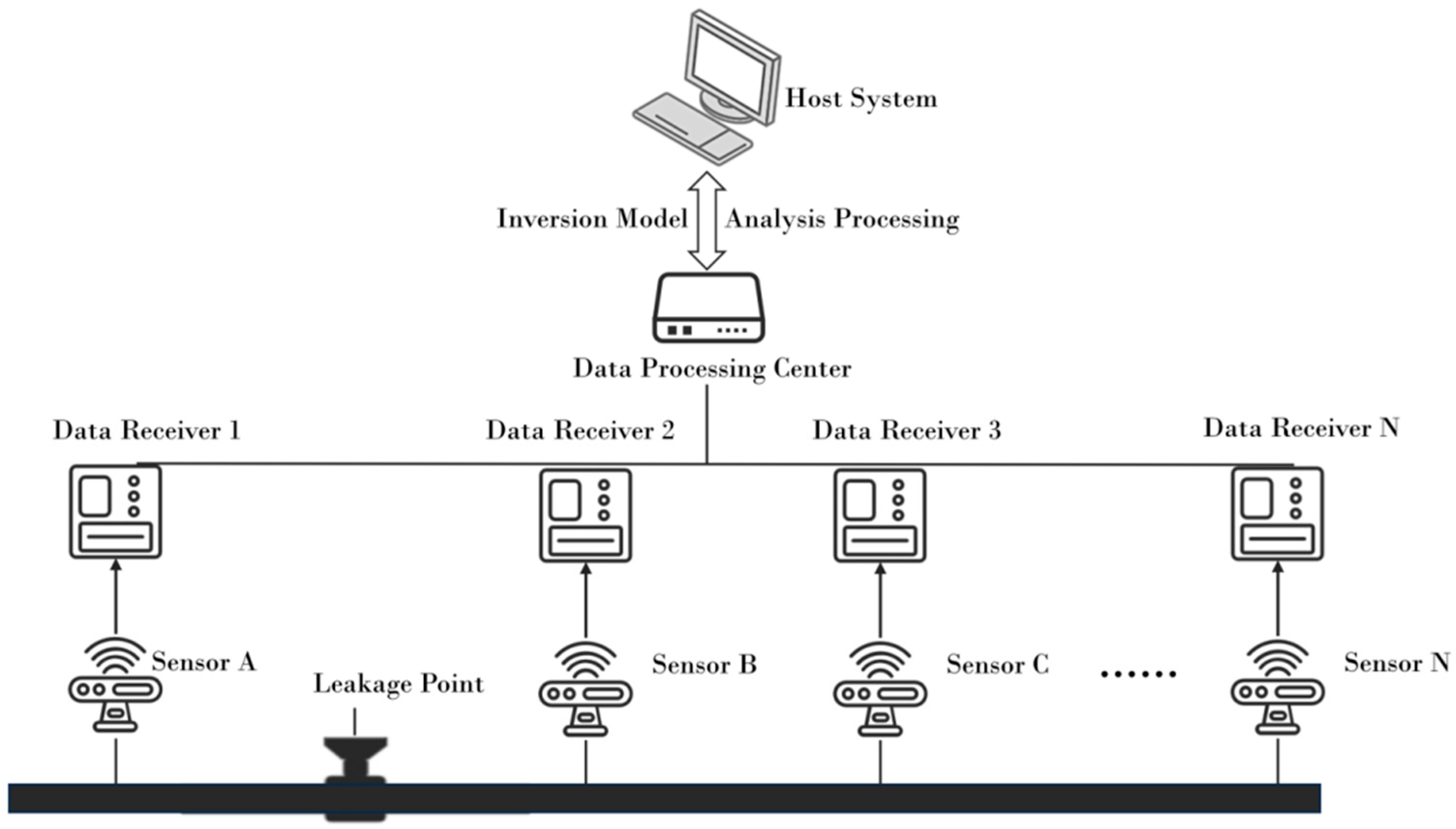
Figure 1. Leakage localization model.
Processes 13 02994 g001
Figure 2. Flowchart of the proposed iterative optimization framework.
Processes 13 02994 g002
Figure 3. Schematic diagram of sensor arrangement for the simulation.
Processes 13 02994 g003
Figure 4. Iterative optimization process of leakage source location and leakage rate based on the Gaussian dispersion model.
Processes 13 02994 g004
Figure 5. Distribution of leaked gas concentration at a height of 1 m on both sides of the pipeline 30 min after leakage.
Processes 13 02994 g005
Figure 6. Comparison of CO2 concentration between the Gaussian dispersion model predictions and those simulated.
Processes 13 02994 g006
Figure 7. Realistic depiction of the experimental setup: (a) front view and (b) side view.
Processes 13 02994 g007
Figure 8. Temporal variation of CO2 concentrations at different downwind distances.
Processes 13 02994 g008
Figure 9. Contour map of CO2 dispersion range.
Processes 13 02994 g009
Figure 10. Comparison of predicted and measured CO2 concentrations as a function of time.
Processes 13 02994 g010
Figure 11. Comparison of predicted and measured peak CO2 concentrations at different monitoring points.
Processes 13 02994 g011
Figure 12. Iterative optimization process of the leak source location and emission rate using data from 10 sensors.
Processes 13 02994 g012
Figure 13. Iterative process of leak emission rate inversion under different numbers of sensors.
Processes 13 02994 g013
Figure 14. Iterative process of leak source location inversion under different numbers of sensors.
Processes 13 02994 g014
Figure 15. Comparison of model prediction errors under different numbers of sensors.
Processes 13 02994 g015
Figure 16. Simulated CO2 concentration evolution under a wind speed of 1 m/s.
Processes 13 02994 g016
Figure 17. Simulated CO2 concentration evolution under a wind speed of 5 m/s.
Processes 13 02994 g017
Table 1. CO2 concentration data detected by each sensor from the FLUENT simulation.
Simulated Sensor ID123456
Coordinates (m)(20, 5, 1)(50, 5, 1)(100, 5, 1)(20, −5, 1)(50, −5, 1)(100, −5, 1)
Concentration (ppm)11,3237136195111,96173992065
Table 2. Briggs diffusion coefficient calculation table.
Atmospheric Stability Classesδy/mδz/m
A0.22α (1 + 0.0001x)−0.50.20α
B0.16α (1 + 0.0001x)−0.50.12α
C0.11α (1 + 0.0001x)−0.50.08α (1 + 0.0002x)−0.5
D0.08α (1 + 0.0001x)−0.50.06α (1 + 0.0015x)−0.5
E0.06α (1 + 0.0001x)−0.50.03α (1 + 0.0003x)−1
F0.04α (1 + 0.0001x)−0.50.016α (1 + 0.0003x)−1
Table 3. Pasquill atmospheric stability classification table.
Wind Speed (m/s)Daytime Solar Radiation IntensityOvercast Daytime or Clear NightCloudy Night (Cloud Cover)
StrongModerateWeak≥5/10≤4/10
<2AA~BBD
2~3A~BBCDEF
3~5BB~CCDDE
5~6CC~DDDDD
>6CDDDDD
Table 4. Error analysis.
ItemSource Strength (kg/s)Leakage Location (m)Concentration at 20 m (ppm)Concentration at 50 m (ppm)Concentration at 100 m (ppm)
Simulated Data3.802.0011,64272682008
Model Prediction3.672.2512,93966011956
Relative Error3.5%12.5%10.0%10.1%2.7%
Table 5. Initial experimental conditions.
ParameterPipeline DiameterCO2 Gas Cylinder
Capacity
Initial PressureLeakage Orifice DiameterLeakage RateWind Speed
Value80 mm25 kg5.85 MPa10 mm0.21 kg/s1.4 m/s
Table 6. Applicable leak source types and concentration distribution characteristics of three common Gaussian dispersion models.
Model TypeApplicable Leak SourceCharacteristicsEngineering Application
Gaussian Plume ModelContinuous sourceForms a stable plume along the wind direction with lateral Gaussian distribution Suitable for long-term continuous leak monitoring and source strength estimation
Gaussian Puff
Model
Point source/Instantaneous releaseInitially high local concentration that disperses over timeApplicable for short-term leak events, emergency response, or theoretical investigations
Gaussian Sphere ModelTheoretical uniform dispersionThree-dimensional spherical symmetry(idealized theoretical model)Suitable for theoretical analysis or model validation; limited practical engineering applications
Disclaimer/Publisher’s Note: The statements, opinions and data contained in all publications are solely those of the individual author(s) and contributor(s) and not of MDPI and/or the editor(s). MDPI and/or the editor(s) disclaim responsibility for any injury to people or property resulting from any ideas, methods, instructions or products referred to in the content.