Abstract
A functional model of a thermoanemometer measuring the air flow velocity on a flat wall surface of the flow has been developed. From the heat balance equation of the sensing elements in the thermoanemometer, a dependence has been derived for determining the heating temperature of the sensing elements. The distribution of the temperature field in the boundary layer was modeled by analogy with the velocity distribution, following a cubic dependence. The distribution of the temperature field on a flat wall surface of the flow from the heating of the sensing elements was obtained analytically by solving the heat conduction equation in the direction of the coordinate of the air flow velocity vector for the boundary conditions of the II as well as II and III kinds. The developed mathematical dependencies enable both the modeling of the distribution of temperature fields in the sensing elements and justifying the distance between them. The reliability of measurements of the air flow velocity on the wall surface of the flow depends on the impossibility of influencing the temperature of one sensing element of the sensor on the temperature of the other. The task of justifying the distance between the sensing elements of the sensor, which are located in the direction of the air flow velocity vector, aims to prevent the interaction of the temperature fields of the elements with each other. The boundary condition is that at the boundary of separation between the temperature fields of the sensing elements, there is a temperature that is 5 to 10% lower than the temperature of the colder sensing element. The ratio of the resistances of the sensing elements is 4/1. The power released by the first sensing element of the sensor, aligned along the air flow velocity vector, is 4 times lower than the heating power of the second sensing element of the sensor. The modeling was carried out at an air flow velocity within 30 and 330 m·s−1. The values of the distances between the sensing elements of the thermal anemometer vary with the supply voltage. The material of the sensing elements is nickel. The contact area of the surface of the sensing elements was 214.337 mm2.
1. Introduction
The use of primary thermoanemometric transducers in flow measurement has become widespread for single-component media. The principle of thermoanemometric measurement of the medium’s mass flow is based on the influence of the fluid flow (in most cases, gas flow) on the heat transfer of the heating element. However, the improvement of thermoanemometric measurement methods focuses on enhancing the design and orientation of sensors within the measuring medium, and there is also the issue of their calibration. Improving the operation of thermoanemometers and their design remains relevant today. In particular, it offers an original design of a thermoanemometer without a Wheatstone measuring bridge [1]. In this case, the temperature of the sensing element (filament) or the current was controlled digitally using a control unit.
Additionally, a method for improving the sensitivity of constant-temperature thermoanemometers has been proposed, which involves the use of an optical fiber with an etched cladding based on a Bragg grating [2]. Experimental studies demonstrated that the sensitivity of the measurement system increased. Schniedenharn et al. suggested an automated system for positioning the thermoanemometer sensor inside the experimental stand [3]. They also proposed several sensor designs for determining gas velocity and other parameters, such as an HWA sensor for measuring velocity and helium concentration in the flow [4]. Furthermore, they developed an HWA sensor capable of measuring velocity, helium concentration, and temperature in helium flows [5]. Similarly, Pantoli et al. designed a sensor that allows simultaneous determination of wind speed and direction for investigating atmospheric flows [6]. A method for producing various HWA sensor designs using 3D printing was also proposed [7]. This approach enables the creation of customized sensor configurations adapted to specific research needs. Atienza et al. presented a film sensor for a constant-temperature thermoanemometer, intended for recording heat transfer in the Martian atmosphere [8]. An actively developing direction in the improvement of measurement systems based on thermoanemometers with heated sensors (HWA) is the use of optical fibers and the Bragg grating effect [9,10]. Optical fibers significantly enhance measurement sensitivity, allowing the detection of even the smallest gas-flow fluctuations. A comparison was carried out between the characteristics of a traditional hot-wire thermoanemometer and an HWA equipped with a fiber-optic sensor [11], for air flow velocities up to 7 m/s.
The results indicated similar data for both approaches, with the fiber-optic sensors showing higher sensitivity. The measurement error did not exceed 10%. For turbomachinery research, a nanoscale probe-type sensor was also proposed [12], which enabled the determination of vortex parameters at the tip. Sadeghi et al. analyzed experimental data on flow velocity obtained using conventional HWA sensors (with a sensing element length of up to 1 mm) and compared them with the results from a nanoscale sensor [13]. Good agreement was achieved between the two sets of results. In flow-velocity studies, resolution, miniaturization, and accuracy of measuring instruments are decisive factors, as they strongly influence micro-scale flows, sonic flows, and turbulent flows [14].
The relevance of research on thermoanemometer-based measurement systems is due to their broad range of applications. These devices are extensively employed in the study of aerodynamics within the aviation sector, particularly for analyzing unsteady flows over aircraft wings or turbulent structures near quadcopter propellers [15,16]. Thermoanemometry also finds wide usage in the energy field, including investigations of pulsating exhaust gas flows in piston engines [17], turbomachinery with continuous flow [18], and vacuum systems [19]. In the automotive industry, hot-wire anemometry (HWA) and various thermal sensors are frequently required to evaluate the cooling efficiency of vented brake disks [20] or to assess noise levels generated by car deflectors [21]. Thermoanemometry is additionally applied in nuclear engineering, for instance, to study convective boiling of liquids [22] or to obtain data on gas dynamics in vertical channels within the cores of prismatic reactors [23]. Thermoanemometers are also utilized to address both classical and fundamental scientific challenges, such as investigating heated shock jets [24], examining the aerodynamic wake behind objects of dissimilar geometries [25,26], and measuring the velocity of a single component in two-phase mixture flows (gas medium and liquid) [27].
Enhancing the electronic circuits and sensor designs of thermoanemometers remains a key objective in advancing thermoanemometry techniques for analyzing the gas-dynamic behavior of liquids and gases. Specifically, the creation of a thermoanemometer capable of measuring air velocity along the boundary layer of streamlined surfaces is crucial for studying flow characteristics over such geometries.
2. Materials and Methods
Let us consider the functional model of a thermoanemometer measuring the air flow velocity on a flat wall surface of the flow. The operation of a thermoanemometer can be described by Equation (1):
where the following terms are defined:
Q is the amount of heat, W; α is the heat transfer coefficient of the sensor element, W/(m2·K);
Sel is the area of the heat transfer surface of the sensor receiving element interacting with the air flow, m2;
Tel and Tar are the temperatures, respectively, of the sensor receiving element and the air flowing around the sensor element, K;
I is the sensor supply current, A;
Rel is the resistance of the sensor receiving element at its temperature, Ω.
Let us simulate the process of heat removal from the sensor receiving elements, provided that air passes past them at the appropriate speed. Figure 1 illustrates the heat flow distribution diagram.
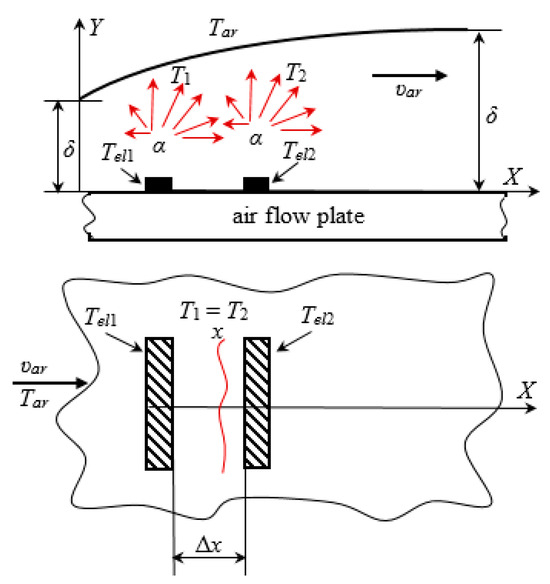
Figure 1.
Scheme of sensor element placement and temperature distribution of the thermoanemometer on the surface of the air flow in the boundary layer.
Two sensing elements are placed on the surface of the air flow plate. Sensor elements in the form of two thin rectangles are placed parallel to each other and perpendicular to the airflow velocity vector. The direction of the air velocity vector υar is co-directed with the X axis.
2.1. Mathematical Model of the Thermoanemometer
The sensor elements are placed on the streamlined plate so that the heat removal by the plate is zero. Ideal thermal insulation of the sensor’s sensing elements to the plate surface. Convective heat transfer is present. The heat balance equation of the sensor elements is written in the form of dependence (2):
where the following terms are defined:
is the amount of heat generated by the sensor’s receiving element;
is the amount of heat taken away by the air flow;
is the amount of heat required to heat the receiving element.
The amount of heat taken away by the air flow is calculated by Formula (3):
The amount of heat required to heat the sensor’s receiving element to the temperature Tel is calculated by the Formula (4):
where the following terms are defined:
m is the mass of the sensor’s receiving element, kg;
is the specific heat capacity of the sensor’s receiving element material, W·kg−1·K−1.
Substitute dependencies (1), (3), and (4) into dependency (2). We obtain the heat balance Equation (5):
From Equation (5), we determine the temperature of the sensor receiving element (6):
Dependence (6) allows us to determine the temperature of the sensor receiving element, taking into account the sensor material, its dimensions, the parameters of the measuring medium, the current and voltage of the sensor supply, and the resistance of the receiving elements. To determine the heat transfer coefficient of the sensor element into the flow medium of the surface, it is necessary to know the distribution of the temperature field in the boundary layer of the flow surface.
2.2. Mathematical Model of Temperature Distribution in the Boundary Layer of a Streamlined Surface
Let us consider a laminar near-wall boundary layer on a flat flow surface. Let the temperature field distribution in the boundary layer have the same form as the velocity distribution [28] in the form of a cubic dependence (7):
where the following terms are defined:
b0, b1, b2, b3 are arbitrary coefficients of Equation (7);
The heat flux in the boundary layer is written as the differential Equation (8) [29]:
where the following terms are defined:
, —velocity according to the coordinate system, m·s−1;
λ—thermal conductivity coefficient, W·s·m−1·K−1;
ρar—density of the flowing medium, kg·m−3;
Car—specific heat capacity of the flowing medium, W·s·kg−1·K−1.
We assume the following initial conditions:
Solve Equation (7) according to the initial conditions (10):
for the initial conditions (9), the second-order differential Equation (7) will be
according to Equation (12), we determine that
In Equation (7), we insert boundary conditions (9), y = 0, T = Tel, we obtain
From Equation (11) and boundary conditions (10), y = δ, T = Tar, dT/dy = 0, we obtain
Substituting boundary conditions (10) into Equation (7), taking into account dependence (14), we obtain expression (15):
From Equation (15), we determine :
Substituting expression (16) into dependence (14), we obtain
Taking into account the dependencies (13), (16), and (17), Equation (7) will have the form:
or Equation (18) in dimensionless parameters will have the form (19):
To calculate the heat transfer coefficient, we use the integral equation of energy conservation (20) [29] (boundary conditions of the II and III kinds):
Let us transform the integral of Equation (20) into an integral of the form (21):
Substitute the expression from Equation (19) into the integral (21), and take into account the dependence (22) for U [28]:
The integral Equation (21) will take the form of Equation (23):
Let us transform Equation (19) into Equation (24):
We take the differential of Equation (24), and we obtain the differential Equation (25):
or
Substituting the right-hand sides of the dependencies (23) and (26) into Equation (20), we obtain the expression (27):
or
The thickness of the boundary near-wall layer is determined by the dependence (29) [29]:
where the following terms are defined:
is the kinematic viscosity of air, m2·s−1;
x is the coordinate in the direction of the air flow vector, m;
is the air velocity at the boundary of the boundary layer, m·s−1.
Taking the differential of Equation (29), we obtain Equation (30):
Taking into account the dependencies (28) and (30), we obtain the dependency (31):
where .
Taking into account the heat conductivity Equation (32) [29]:
and dependency (26), and disregarding the minus sign, we obtain Equation (33):
The solution of the polynomial Equation (31) gives a value that can be used for the thermal boundary layer. If we consider that δT = δ = 1, then the ratio 31/420 = 0.074 is a second-order quantity after the integer value of the number; therefore, can be neglected.
Then, from Equation (31), we obtain the dependence (34):
where Pr is the Prandtl criterion.
Taking into account the dependence (34) and the dependence (33), the heat transfer coefficient is calculated by the dependence (35):
From Equation (29), we calculate the dynamic boundary layer and substitute it into Equation (35), and we obtain Equation (36):
Equation (36) enables us to model the heat transfer coefficient of the sensing element in the thermoanemometer sensor as a function of air flow velocity and the physical properties of the air.
2.3. Justification of the Spacing Between the Sensing Elements of the Sensor
The placement of the sensor’s sensing elements on the surface of the plate, which is flowed by air, is given by the parameter, the distance between the sensing elements. The distance between the sensing elements depends on the power supplied to the sensing elements, the thermal characteristics of the air, and the material of the sensing elements.
The condition for the accuracy of measuring the air flow velocity is the absence of mutual influence of the temperature fields of the sensing elements. We assume the condition that there is a boundary of the temperature field where the temperature is equal to the temperature of the colder sensing element.
The amount of heat released by the sensing element is determined by the Formula (37):
where UR is the supply voltage of the sensing element, V.
The intensity of heat release per unit volume, where the heat flux is distributed, is q/ΔV, where ΔV represents the increase in volume of the space in which the heat flux is distributed.
The increase in the volume of the space in which the heat flow is distributed is calculated by the Formula (38):
where Lz is the length of the receiving element in the direction perpendicular to the air flow velocity vector.
The differential equation for the temperature field distribution is written as Equation (39) (for boundary conditions of the II and III kinds):
Integrating Equation (39):
The constant of integration C1 is determined from the boundary conditions of the boundary layer at x = 0, which corresponds to condition (41) (boundary conditions of the II kind):
The integration constant, taking into account Equations (40) and (41), will be determined by the dependence (42):
Integrating Equation (40), taking into account the integration constant expression (42), we obtain the temperature distribution Equation (43):
From the boundary conditions, at x = 0, T = Tel, we determine the constant of integration C2 (44):
Taking into account the dependence (44), Equation (43) for a receiving ring with resistance Rel1 will take the form:
where the dependence of from Equation (6) will be
For a receiving ring with resistance Rtl2,
where the dependence of from Equation (6) will be
The resistance ratio of the sensing elements is 4/1. The power released by the first sensing element of the sensor along the air flow velocity vector is 4 times lower than the heating power of the second sensing element of the sensor.
The task of justifying the distance between the sensing elements of the sensor, which are placed in the direction of the air flow velocity vector, aims to prevent the interaction of the temperature fields of the elements with each other.
3. Results
3.1. Distribution of the Temperature Field of the Sensing Elements of the Thermoanemometer in the Near-Wall Surface of the Boundary Layer of Air Flow
To heat the sensors, the supply voltage of the bridge circuit was assumed to be 2 V. The resistance of the first sensing element was Rel2 = 0.06 Ω, and the resistance of the second sensing element was Rel1 = 0.015 Ω. Accordingly, the heat flux power on the first sensor element was 66.67 W, and on the second, 266.67 W. The simulation results for the sensor element with resistance Rel1 = 0.06 Ω are shown in Figure 2a, and for the sensor element with resistance Rel2 = 0.015 Ω are shown in Figure 2b.
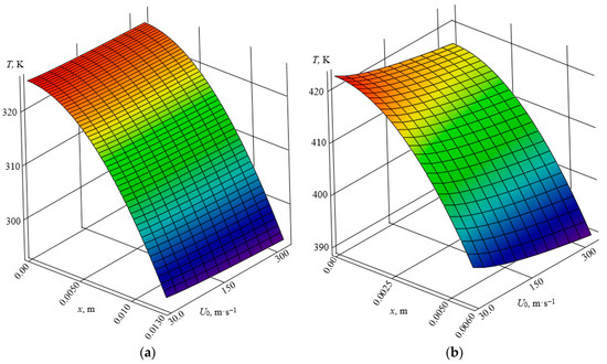
Figure 2.
Distribution of the temperature field of the sensor receiving element for the element resistance Rel and the supply voltage 2 V, depending on the speed U0 of the air flow around the surface and the distance x from the element: (a) Rel1 = 0.06 Ω; (b) Rel2 = 0.015 Ω.
The sensor element with a heat flux power of 66.667 W heats up to a temperature of 325.67 K (Figure 2a). The second sensor element, with a resistance 4 times lower, develops a power of 266.667 W and heats up to a temperature of 422.8 K (Figure 2b). The distribution of the temperature field from the element with a higher heating temperature changes depending on the velocity of the air flow around the element. With increasing velocity, the temperature field decreases more intensively (Figure 2b) than the colder element (Figure 2a).
The distance of the temperature field displacement for the receiving element with a resistance of 0.06 Ω in the direction of the air flow velocity vector to the temperature of the incoming air is 13 mm. The distance of the temperature field displacement for the receiving element with a resistance of 0.015 Ω in the direction of the air flow velocity vector depends on the speed of the air flow. At an air flow velocity of 30 m·s−1, the air temperature at a distance of 16 mm from the sensing element will be 320 K. At an air flow velocity of 300 m·s−1, the air temperature at a distance of 16 mm from the sensing element will be 293.8 K.
3.2. Modeling the Air Temperature at the Boundary of the Temperature Fields of the Sensing Elements of the Thermoanemometer in the Near-Wall Surface of the Boundary Layer of the Air Flow
The reliability of air flow velocity measurements on the near-wall surface of the flow depends on the impossibility of the temperature of one sensing element of the sensor affecting the temperature of the other. We assume the boundary condition that at the boundary of the separation of the temperature fields of the sensing elements, there is a temperature 5–10% lower than the temperature of the colder sensing element.
The modeling of the boundary of separation of temperature fields of the sensing elements was carried out in the absence of air flow (Figure 3a) and the presence of air flow velocity on the distribution of the thermal field for the sensing element with a higher heating temperature (Figure 3b). The parameters are the same as those used in the modeling of temperature fields; the methodology is outlined in Section 2.3.
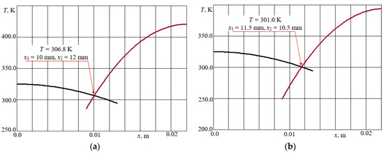
Figure 3.
Temperature field boundaries of the sensor sensing elements for element resistance Rel (Rel1 = 0.06 Ω—lower element heating temperature, Rel2 = 0.015 Ω—higher element heating voltage) and supply voltage 2 V when air flows around the surface at a speed var = 100 m·s−1 for boundary conditions: (a) II kind; (b) II and III kinds.
For boundary conditions of II kind (Figure 3a), the temperature at the boundary of the temperature field was assumed to be 306.8 K. The distance to the boundary with a temperature of 306.8 K from the first sensing element in the direction of the air velocity vector is x1 = 10 mm. The distance from the second sensing element in the direction opposite to the air velocity vector is x2 = 12 mm. The distance between the sensing elements is Δx = 22 mm.
For the boundary conditions of the II and III kinds (Figure 3b), provided that the distance between the sensing elements is maintained at 22 mm, the temperature at the boundary of the temperature fields will be 301 K. The distances to the boundary of the temperature fields, respectively, from the first sensing element, x1 = 11.5 mm, and from the second sensing element, x2 = 10.5 mm.
The simulation was performed at an air flow velocity of 100 m·s−1 at the near-wall surface of the flow.
To determine the influence of air flow velocity on the temperature at the boundary of the temperature fields and the distance between the sensing elements of the thermoanemometer, the simulation was performed at an air flow velocity of 300 m·s−1 near the wall surface of the flow (var = 300 m·s−1; Figure 4).
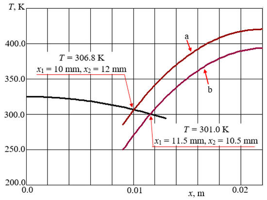
Figure 4.
Limits of temperature fields of the sensor’s sensing elements for the element resistance Rel (Rel1 = 0.06 Ω—lower element heating temperature, Rel2 = 0.015 Ω—higher element heating voltage) and supply voltage 2 V when air flows around the surface at a speed of var = 300 m·s−1 for boundary conditions of the II kind (a) and II and III kinds (b).
The parameters of the boundary of the temperature field distribution are the same as at the air flow velocity var = 100 m·s−1 (Figure 4).
4. Discussion
Analysis of the Results of Modeling the Temperature Parameters of the Sensing Elements of the Thermoanemometer
Medium flow velocity sensors are mainly used for flows in round-section wires or wires of other cross-sectional configurations. With an increase in the flow velocity of the medium flowing around the surface of the sensing elements of the thermoanemometer, the temperature of these elements decreases at a constant supply voltage (Figure 5). This was also demonstrated by previous studies on flow meters, including the flow of a homogeneous medium in a pipe [30], the flow of a two-phase medium in a pipe [27], and the flow of a homogeneous medium over a horizontal surface [31]. The change in heating temperature of the sensing elements in the thermoanemometer, as a function of air flow velocity, is shown in Figure 5.
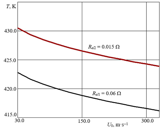
Figure 5.
Dependence of the heating temperature of the sensing elements of the thermoanemometer on the speed of air flow around the surface.
The heating power of the sensing elements of the thermoanemometer determines the distance between them. For the sensing elements of the thermoanemometer, with resistances of 0.06 Ω and 0.015 Ω and a supply voltage of 2 V, the rational distance between them should be 22 mm. With a decrease in heating power, the distance between the sensing elements when they are installed on a horizontal surface decreases.
Figure 6 illustrates the heating temperature of the sensing elements in the thermoanemometer as a function of the supply voltage.
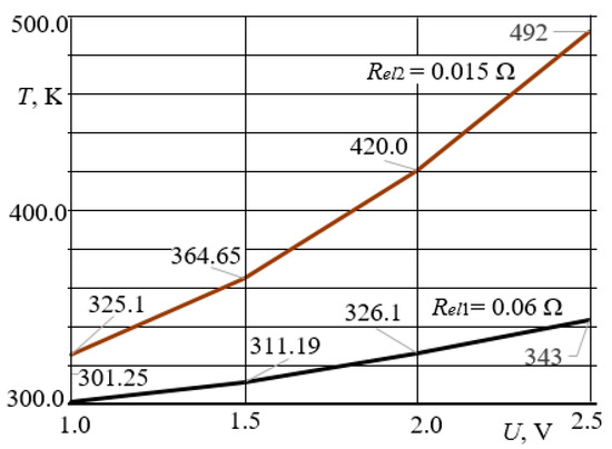
Figure 6.
Dependence of the temperature T of the heating of the sensing elements of the thermoanemometer on the supply voltage U.
At a supply voltage U = 1 V, the power on the sensing elements will be 16.67 W and 67.67 W, respectively. The sensing elements will heat up to a temperature of 302.25 K and 325.1 K, respectively. At a supply voltage U = 2.5 V, the power on the sensing elements will be 104.17 W and 416.67 W, respectively. The sensing elements are heated to temperatures of 343.0 K and 492.0 K, respectively.
A change in the heating temperature of the elements leads to a change in the distance between them (Figure 7).
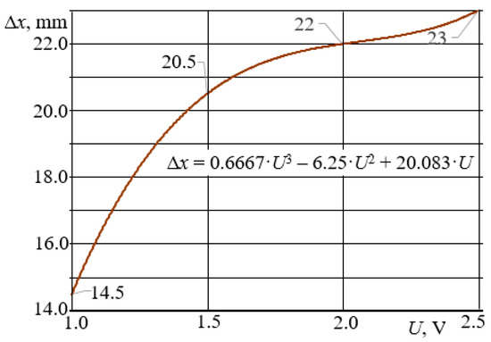
Figure 7.
Dependence of the distance Δx of the placement of the sensing elements of the thermoanemometer on the supply voltage U.
The modeling of the distance between the placement of the sensing elements was carried out for the boundary conditions of the second kind, and the temperature at the boundary of the temperature field was assumed to be 306.8 K. For the boundary conditions of the II and III kinds, provided that the distance between the sensing elements is maintained, the temperature at the boundary of the separation of the temperature fields was assumed to be 301 K. At the supply voltage U = 1 V, the distance between the sensing elements of the thermoanemometer under the given boundary conditions is Δx = 14.5 mm. Accordingly, at a supply voltage of U = 1.5 V, the distance between the sensing elements is Δx = 20.5 mm, and at a supply voltage of U = 2.5 V, the distance between the sensing elements is Δx = 23 mm.
The nature of the change in the distance between the sensing elements of the thermoanemometer, depending on the supply voltage, is nonlinear and is described by the cubic dependence (49):
The nonlinear characteristic of the change in distance between the sensing elements of the thermoanemometer is due to the nonlinear heat transfer characteristics of the sensing elements to the medium flowing around them. This was confirmed by previous studies, which used a liquid as the flow medium [27,32].
5. Conclusions
The heating power of the sensing elements of the thermoanemometer affects the distance between the elements. The dependence of the distance on the supply voltage (heating power) is nonlinear. As the element temperature increases, the distance between them changes according to a cubic dependence. The distance between the sensing elements is justified as 22 mm. The supply voltage is 2 V, and the material of the sensing elements is nickel. Their resistances are 0.06 Ω and 0.015 Ω, respectively. The placement of the sensing elements in the direction of the air flow velocity vector from the lower temperature to the higher temperature of the elements.
The temperature at the boundary of the temperature fields and the distance of the field boundary from the sensing elements of the thermoanemometer are variable depending on the air flow velocity, the distance between the elements, and the power supplied to the sensor elements. In real time, the boundary of the temperature field will be dynamic, and displacement in the flow direction will occur depending on the speed and amount of the measuring medium, as well as the nature of the movement.
Compensation for dynamic fluctuations of the temperature field boundary can be performed by the measurement circuit using voltage feedback compensation in the power control circuit for the sensing elements of the thermoanemometric sensor. Alternating current in the kilohertz range is used.
Author Contributions
Conceptualization, T.D., V.D. and M.B.; Methodology, T.D. and M.B.; Software, T.D.; Validation, T.D., V.D. and M.B.; Formal analysis, V.D.; Investigation, T.D.; Resources, M.B.; Data curation, V.D.; Writing—original draft, T.D.; Writing—review & editing, T.D. and M.B.; Supervision, V.D.; Project administration, M.B. All authors have read and agreed to the published version of the manuscript.
Funding
This research received no external funding.
Data Availability Statement
The original contributions presented in this study are included in the article. Further inquiries can be directed to the corresponding authors.
Acknowledgments
The results presented in the article will be a part of Taras Dmytriv’s Ph.D. thesis.
Conflicts of Interest
The authors declare no conflicts of interest.
References
- Gomes, R.A.; Niehuis, R. Development of a novel anemometry technique for velocity and temperature measurement. Exp. Fluids. 2018, 59, 142. [Google Scholar] [CrossRef]
- Tang, Y.; Chen, X.; Zhang, J.; Xiong, L.; Dong, X. Sensitivity-Enhanced Hot-Wire Anemometer by Using Cladding-Etched Fiber Bragg Grating. Photonic Sens. 2023, 13, 230305. [Google Scholar] [CrossRef]
- Schniedenharn, M.; Wiedemann, F.; Schleifenbaum, J.H. Visualization of the shielding gas flow in SLM machines by space-resolved thermal anemometry. Rapid Prototyp. J. 2018, 24, 1296–1304. [Google Scholar] [CrossRef]
- Hewes, A.; Mydlarski, L. Design of thermal-anemometry-based probes for the simultaneous measurement of velocity and gas concentration in turbulent flows. Meas. Sci. Technol. 2021, 32, 105305. [Google Scholar] [CrossRef]
- Hewes, A.; Mydlarski, L. Simultaneous measurements of velocity, gas concentration, and temperature by way of thermal-anemometry-based probes. Meas. Sci. Technol. 2022, 33, 015301. [Google Scholar] [CrossRef]
- Pantoli, L.; Paolucci, R.; Muttillo, M.; Fusacchia, P.; Leoni, A. A multisensorial thermal anemometer system. Lect. Notes Electr. Eng. 2018, 431, 330–337. [Google Scholar] [CrossRef]
- Daniel, F.; Peyrefitte, J.; Radadia, A.D. Towards a completely 3D printed hot wire anemometer. Sens. Actuators A Phys. 2020, 309, 111963. [Google Scholar] [CrossRef]
- Atienza, M.-T.; Kowalski, L.; Gorreta, S.; Jiménez, V.; Domínguez-Pumar, M. Thermal dynamics modeling of a 3D wind sensor based on hot thin film anemometry. Sens. Actuators A Phys. 2018, 272, 178–186. [Google Scholar] [CrossRef]
- De Vita, E.; Di Palma, P.; Zahra, S.; Roviello, G.; Ferone, C.; Iadicicco, A.; Campopiano, S. Hot-wire anemometer based on D-shaped Optical Fiber. IEEE Sens. J. 2023, 23, 12845. [Google Scholar] [CrossRef]
- Zhang, J.; Tang, Y.; Xu, P.; Xu, O.; Dong, X. Intensity-interrogated hot-wire anemometer based on chirp effect of a fiber Bragg grating. Opt. Express 2022, 30, 37124–37130. [Google Scholar] [CrossRef] [PubMed]
- Sekine, M.; Furuya, M. Development of Measurement Method for Temperature and Velocity Field with Optical Fiber Sensor. Sensors 2023, 23, 1627. [Google Scholar] [CrossRef] [PubMed]
- Pique, A.; Miller, M.A.; Hultmark, M. Characterization of the wake behind a horizontal-axis wind turbine (HAWT) at very high Reynolds numbers. J. Phys. Conf. Ser. 2020, 1618, 062039. [Google Scholar] [CrossRef]
- Sadeghi, H.; Lavoie, P.; Pollard, A. Effects of finite hot-wire spatial resolution on turbulence statistics and velocity spectra in a round turbulent free jet. Exp. Fluids. 2018, 59, 40. [Google Scholar] [CrossRef]
- Takegawa, N.; Ishibashi, M.; Iwai, A.; Furuichi, N.; Morioka, T. Verification of flow velocity measurements using micrometer-order thermometers. Sci. Rep. 2021, 11, 23778. [Google Scholar] [CrossRef]
- Chen, S.; Shi, Z.; Geng, X.; Zhao, Z.; Chen, Z.; Sun, Q. Study of the transient flow structures generated by a pulsed nanosecond plasma actuator on a delta wing. Phys. Fluids. 2022, 34, 107111. [Google Scholar] [CrossRef]
- Tofan-Negru, A.; Ștefan, A.; Grigore, L.Ú.; Oncioiu, I. Experimental and Numerical Considerations for the Motor-Propeller Assembly’s Air Flow Field over a Quadcopter’s Arm. Drones. 2023, 7, 199. [Google Scholar] [CrossRef]
- Simonetti, M.; Caillol, C.; Higelin, P.; Dumand, C.; Revol, E. Experimental investigation and 1D analytical approach on convective heat transfers in engine exhaust-type turbulent pulsating flows. Appl. Therm. Eng. 2020, 165, 114548. [Google Scholar] [CrossRef]
- Silva, R.L.; Brito, S.X. Experimental evaluation of energy efficiency and velocity fields on a low-pressure axial flow fan (desktop type). Energy Effic. 2019, 12, 697–710. [Google Scholar] [CrossRef]
- Dmytriv, V.T.; Dmytriv, I.V.; Borovets, V.M.; Horodetskyy, I.M.; Kachmar, R.Y.; Dmyterko, P.R. Analytical-experimental studies of delivery rate and volumetric efficiency of rotor-type vacuum pumps for milking machine. INMATEH—Agric. Eng. 2019, 58, 57–62. [Google Scholar]
- Bombek, G.; Hribernik, A. Flow behaviour in vented brake discs with straight and airfoil-shaped radial vanes. Proc. Inst. Mech. Eng. Part D J. Automob. Eng. 2022, 237, 3448–3464. [Google Scholar] [CrossRef]
- Sip, J.; Lizal, F.; Pokorny, J.; Elcner, J.; Jedelsky, J.; Jicha, M. Automotive cabin vent: Comparison of RANS and LES approaches with analytical-empirical equations and their validation with experiments using Hot-Wire Anemometry. Build. Environ. 2023, 233, 110072. [Google Scholar] [CrossRef]
- Francois, F.; Djeridi, H.; Barre, S.; Klédy, M. Measurements of void fraction, liquid temperature and velocity under boiling two-phase flows using thermal-anemometry. Nucl. Eng. Des. 2021, 381, 111359. [Google Scholar] [CrossRef]
- Taha, M.M.; Said, I.A.; Zeitoun, Z.; Usman, S.; Al-Dahhan, M.H. Effect of non-uniform heating on temperature and velocity profiles of buoyancy driven flow in vertical channel of prismatic modular reactor core. Appl. Therm. Eng. 2023, 225, 120209. [Google Scholar] [CrossRef]
- Antošová, Z.; Trávníček, Z. Stagnation Point Heat Transfer to an Axisymmetric Impinging Jet at Transition to Turbulence. J. Heat Transf. 2023, 145, 023902. [Google Scholar] [CrossRef]
- Faria, A.F.; Avelar, A.C.; Francisco, C.P.F. Transient experimental analysis in the wake of bluff bodies. J. Braz. Soc. Mech. Sci. Eng. 2023, 45, 100. [Google Scholar] [CrossRef]
- Hajimirzaie, S.M. Experimental Observations on Flow Characteristics around a Low-Aspect-Ratio Wall-Mounted Circular and Square Cylinder. Fluids 2023, 8, 32. [Google Scholar] [CrossRef]
- Dmytriv, V.; Dmytriv, I.; Dmytriv, T. Research in thermoanemometric measuring device of pulse flow of two-phase medium. Eng. Rural Dev. 2018, 17, 898–904. [Google Scholar] [CrossRef]
- Dmytriv, T.V.; Mykyychuk, M.M.; Dmytriv, V.T. Analytical model of dynamic boundary layer on the surface under laminar flow mode. Mach. Energetics 2021, 12, 93–98. (In Ukrainian) [Google Scholar] [CrossRef]
- Carslaw, H.S.; Jaeger, J.C. Conduction of Heat in Solids; Oxford University Press: New York, NY, USA, 1959. [Google Scholar]
- Cebula, A. Experimental and numerical investigation of thermal flow meter. Arch. Thermodyn. 2015, 36, 149–160. [Google Scholar] [CrossRef][Green Version]
- Diwate, M.; Tawade, J.V.; Janthe, P.G.; Garayev, M.; El-Meligy, M.; Kulkarni, N.; Gupta, M.; Ijaz Khan, M. Numerical solutions for unsteady laminar boundary layer flow and heat transfer over a horizontal sheet with radiation and nonuniform heat Source/Sink. J. Radiat. Res. Appl. Sci. 2024, 17, 101196. [Google Scholar] [CrossRef]
- Dmytriv, V. Model of forced turbulence for pulsing flow. Diagnostyka 2020, 21, 89–96. [Google Scholar] [CrossRef]


Disclaimer/Publisher’s Note: The statements, opinions and data contained in all publications are solely those of the individual author(s) and contributor(s) and not of MDPI and/or the editor(s). MDPI and/or the editor(s) disclaim responsibility for any injury to people or property resulting from any ideas, methods, instructions or products referred to in the content. |
© 2025 by the authors. Licensee MDPI, Basel, Switzerland. This article is an open access article distributed under the terms and conditions of the Creative Commons Attribution (CC BY) license (https://creativecommons.org/licenses/by/4.0/).