Article

A Non-Destructive Deep Learning–Based Method for Shrimp Freshness Assessment in Food Processing

by
Dongyu Hao
1,
Cunxi Zhang
2,*,
Rui Wang
2,
Qian Qiao
1,
Linsong Gao
1,
Jin Liu
1 and
Rongsheng Lin
3
1
School of Marine Engineering Equipment, Zhejiang Ocean University, Zhoushan 316022, China
2
School of Naval Architecture and Maritime, Zhejiang Ocean University, Zhoushan 316022, China
3
Jurong Energy (Xinjiang) Co., Ltd., Kazak Autonomous Prefecture of Ili 841600, China
*
Author to whom correspondence should be addressed.
Processes 2025, 13(9), 2895; https://doi.org/10.3390/pr13092895
Submission received: 8 August 2025 / Revised: 26 August 2025 / Accepted: 27 August 2025 / Published: 10 September 2025
(This article belongs to the Section Food Process Engineering)

Abstract

Maintaining the freshness of shrimp is a critical issue in quality and safety control within the food processing industry. Traditional methods often rely on destructive techniques, which are difficult to apply in online real-time monitoring. To address this challenge, this study aims to propose a non-destructive approach for shrimp freshness assessment based on imaging and deep learning, enabling efficient and reliable freshness classification. The core innovation of the method lies in constructing an improved GoogLeNet architecture. By incorporating the ELU activation function, L2 regularization, and the RMSProp optimizer, combined with a transfer learning strategy, the model effectively enhances generalization capability and stability under limited sample conditions. Evaluated on a shrimp image dataset rigorously annotated based on TVB-N reference values, the proposed model achieved an accuracy of 93% with a test loss of only 0.2. Ablation studies further confirmed the contribution of architectural and training strategy modifications to performance improvement. The results demonstrate that the method enables rapid, non-contact freshness discrimination, making it suitable for real-time sorting and quality monitoring in shrimp processing lines, and providing a feasible pathway for deployment on edge computing devices. This study offers a practical solution for intelligent non-destructive detection in aquatic products, with strong potential for engineering applications.

1. Introduction

Shrimp has gained global popularity due to its high nutritional value, including rich protein content [1]. It is also an important source of omega-3 fatty acids, essential for maintaining human health [2]. The consumption and market demand for shrimp continue to grow, highlighting the importance of ensuring its quality and freshness [3]. However, shrimp quality quickly deteriorates due to microbial contamination [4]. Additionally, endogenous enzymatic activities accelerate spoilage, further complicating preservation efforts. Maintaining freshness throughout distribution remains a critical challenge for the seafood industry [5]. Traditional methods for evaluating shrimp freshness often rely on sensory evaluations, which can lbe subjective and unreliable [6]. Chemical and microbiological tests, while accurate, are typically slow and complex, unsuitable for rapid freshness evaluation [7,8].
To address these limitations, modern techniques utilizing machine learning and computer vision have emerged as viable alternatives [9]. Convolutional neural networks (CNNs) in particular have shown exceptional accuracy in freshness detection, providing efficient and reliable assessments [10]. CNN-based methods excel in extracting image features essential for precise freshness evaluation [11]. Despite their strengths, CNN models face computational complexity and overfitting risks, particularly with limited datasets [12]. To mitigate these challenges, transfer learning has become an effective approach to enhance model robustness and generalization [13]. Advanced CNN architectures like GoogLeNet have been optimized to further improve freshness detection performance [14].
Recent studies have further reinforced the potential of artificial intelligence in seafood quality monitoring. For instance, machine vision techniques combined with deep learning models have shown remarkable results in grading fish freshness, texture, and spoilage indicators [15]. Moreover, the fusion of multispectral imaging and deep neural networks has been explored to enhance classification performance in freshness prediction tasks [16]. Compared to traditional RGB imaging [17], multispectral data enables more robust feature extraction across different wavelengths, contributing to higher accuracy and better generalization. In shrimp freshness evaluation specifically, attention mechanisms and lightweight CNN architectures are being applied to reduce computational cost while maintaining accuracy [18,19]. These approaches are increasingly suitable for embedded systems and real-time applications.
Nevertheless, challenges remain in ensuring robustness and generalizability due to inter-sample variability caused by species, environmental, and logistical differences [20]. To overcome this, ensemble learning and hybrid modeling frameworks integrating both image and physicochemical data are being explored [21]. To meet the need for rapid and objective decisions on shrimp processing lines, we develop a non-destructive, image-driven freshness assessment model built upon GoogLeNet. The core novelty of the model is reflected in the following aspects: firstly, the original ReLU activation function is replaced with ELU to improve gradient flow and enhance feature representation capability; secondly, L2 regularization is introduced along with an additional fully connected layer to strengthen the model’s generalization ability; finally, transfer learning combined with the RMSProp optimizer is employed to effectively mitigate overfitting under limited sample conditions. Systematic experiments demonstrate that the model achieves high classification accuracy and convergence efficiency on the shrimp image dataset, outperforming several CNN baseline models. These findings contribute to advancing process-oriented quality monitoring research. The improvements enhance generalization capacity and reduce overfitting in small-sample scenarios. Experimental results indicate that the proposed method surpasses comparative CNN baselines in terms of accuracy, convergence efficiency, and robustness.
The objective of this study is to establish a real-time, non-destructive freshness assessment method suitable for shrimp processing lines, capable of supporting online sorting and deployment on edge devices, thereby providing a reliable technical solution for intelligent quality monitoring in the seafood industry.

2. Materials and Methods

2.1. Shrimp Sample Collection

In this study, fresh marine shrimp purchased from the seafood market in Zhoushan, Zhejiang Province, China were used as experimental samples, with a total of 500 shrimp and an average body weight of 20 ± 5 g. After purchase, the shrimp samples were immediately placed in a constant-temperature refrigeration unit (Haier Group, Qingdao, China), which was strictly maintained at 0 °C to simulate the actual cold-chain transportation and storage conditions of aquatic products. To establish an accurate and reliable standard for freshness evaluation, starting from the first day of storage, 4 shrimp were randomly selected at 20:00 every day for physicochemical analysis, specifically to determine the content of total volatile basic nitrogen (TVB-N). The TVB-N determination was performed using a Kjeldahl nitrogen analyzer (FOSS Analytical, Hillerød, Denmark), combined with a total volatile basic nitrogen detection kit (Laboratory of Fisheries College, Zhejiang Ocean University, Zhoushan, China) to ensure the accuracy of the detection results. This determination was conducted continuously for 13 days, and a total of 52 clear TVB-N values were finally obtained, serving as representative physicochemical reference data [22].
At the same time, standardized image acquisition was carried out on the remaining samples at the exact same time point (20:00) as the TVB-N determination: during the acquisition process, LED fill lights (Philips, Amsterdam, the Netherlands) were used to provide a stable light source to ensure consistent lighting conditions; a Canon EOS 90D digital camera (Canon Inc., Tokyo, Japan) was used for shooting. No data augmentation or post-processing was performed during the acquisition of all images to ensure the independence and authenticity of visual features in each image. This study strictly follows the standard methods in the field of food quality visual evaluation, which assumes that shrimp stored under the same conditions and sampled at the same time point have similar physicochemical properties [23]. Therefore, the TVB-N value determined each day was used as a unified reference label for all images acquired on that day. This method has been widely applied in deep learning-based food quality evaluation and freshness classification of agricultural products, and has been verified by a number of high-level studies [24].
It should be noted that although the above experimental design assumes that "samples stored under the same conditions and sampled at the same time point have comparable physicochemical properties", inter-individual biological variability cannot be completely eliminated. Potential sources of variation include differences in body weight, genetic background, feeding history, and initial microbiota, which may affect spoilage kinetics and thus alter freshness indicators [25]. To mitigate these effects, this study controlled the sample body weight range (20 ± 5 g), implemented daily random sampling and repeated TVB-N determinations, and maintained a unified processing protocol at 0 °C with a fixed daily sampling time. In addition, since TVB-N determination is a destructive and labor-intensive chemical analysis method, a balanced daily replicate number of n = 4 was adopted in this study to balance statistical comparability and complete time-series coverage. This range of replicates (approximately 3–6 biological replicates per time point) is consistent with common practices in the field of aquatic product freshness research [26,27].
Furthermore, a date-stratified image dataset (1746 images) was constructed and uniformly labeled with the corresponding daily TVB-N value, enabling the classification model to learn and smooth within-day natural variation while maintaining a unified physicochemical label. Residual inter-individual heterogeneity is acknowledged as a limitation and is discussed in the manuscript. Subsequently, the dataset was partitioned into training and test sets according to stringent data-splitting criteria and used to construct and validate a deep learning–based shrimp freshness recognition model.

2.2. Image Acquisition and Preprocessing

The image acquisition system used in this experiment consisted of a high-resolution camera, a uniform lighting source, and a stable experimental platform. The distance between the camera and the shrimp samples was approximately 30 cm, chosen to simulate varying experimental conditions and generate representative data. The image acquisition setup is shown in Figure 1. This distance was selected to reflect potential variability in practical scenarios, ensuring that the dataset covers diverse experimental conditions. All images were captured under controlled lighting to ensure high-quality shrimp images suitable for subsequent image processing and deep learning model training.

2.3. Data Augmentation

Due to the limited number of original image samples, directly training a deep learning model may lead to overfitting. To improve the generalization ability of the model, data augmentation techniques were applied to expand the dataset. The main augmentation operations included image rotation, horizontal flipping, brightness adjustment, and contrast variation. As a result of data augmentation, a total of 5890 high-quality shrimp images were obtained for model training and testing.

2.4. Freshness Level Classification

Shrimp freshness was graded using the physicochemical indicator total volatile basic nitrogen (TVB–N). According to the Chinese aquatic industry standard SC/T 3113–2002 (Frozen Shrimp) and the Chinese national standard GB 2733–2015 (Fresh and Frozen Animal Aquatic Products) [28,29], the thresholds were: Grade I (excellent) 20 mg N / 100 g ; Grade II (good) ( 20 , 25 ] mg N / 100 g ; Grade III (qualified/marginal) ( 25 , 30 ] mg N / 100 g ; and Non-conforming (inedible) > 30 mg N / 100 g . Under storage at 0 °C, TVB–N increased slowly at first; samples were Grade I on days 0–6, then Grade II on days 7–9, Grade III on days 10–12, and Non-conforming on day 13 when TVB–N exceeded 30 mg N / 100 g (Figure 2).
An image dataset was constructed by assigning to each image the day-specific TVB–N grade under strictly controlled imaging conditions. The final dataset contains n = 7380 valid samples, with the following per-class totals (Table 1): Grade I = 2616 ( 35.45 % ), Grade II = 1380 ( 18.70 % ), Grade III = 1836 ( 24.86 % ), and Non-conforming = 1548 ( 20.97 % ). A moderate class skew was quantified by the imbalance ratio
IR = max c n c min c n c ,
To mitigate potential bias, three safeguards were adopted: (i) a stratified train/test split to preserve per-class proportions; (ii) a class-weighted negative log-likelihood loss with weights inversely proportional to class frequency,
w c = N C n c ,
L = i = 1 N c = 1 C w c y i , c log p ^ i , c ;
and (iii) reporting macro-precision, macro-recall, macro-F1, and Cohen’s κ in addition to overall accuracy to avoid dominance by majority classes. With these controls, the TVB–N labeling remains consistent and reproducible across the dataset, providing a stable and reliable supervision signal for model training and evaluation.

2.5. Models and Improvements

2.5.1. GoogLeNet Architecture and Applicability Analysis

In this study, GoogLeNet was selected as the base model. By incorporating residual modules, the network depth is increased while effectively preventing gradient vanishing. The overall framework of the proposed approach is shown in Figure 3. After image acquisition, the data undergoes preprocessing and augmentation. Images are then classified into freshness levels based on physicochemical indicators. The base network is subsequently optimized and improved to build a high-performance model, which is finally deployed on mobile devices.
GoogLeNet is a deep convolutional neural network model proposed by the Google team. It achieved outstanding performance in the 2014 ImageNet Large-Scale Visual Recognition Challenge and attracted widespread attention. The design philosophy of GoogLeNet is distinctive, emphasizing a balance between network depth and computational efficiency. It introduced the Inception module and brought innovations to network architecture, as shown in Figure 4.
The Inception block contains four parallel branches. The first three branches use convolutional layers with kernel sizes of 1 × 1, 3 × 3, and 5 × 5, respectively, to extract features at different spatial scales. In the second and third branches, a 1 × 1 convolution is first applied to reduce the number of input channels, thereby lowering the model’s complexity. The fourth branch uses a 3 × 3 max pooling layer followed by a 1 × 1 convolution to adjust the number of output channels. All four branches use appropriate padding to ensure that the height and width of the outputs are consistent with those of the input. Finally, the outputs of the four branches are concatenated along the channel dimension and passed forward in the network.
Google initially proposed the original Inception structure, which stacks commonly used convolutional operations in CNNs—1 × 1, 3 × 3, and 5 × 5 convolutions—along with 3 × 3 max pooling. By maintaining the same spatial dimensions through padding and summing the feature maps along the channel axis, the module increases both the width of the network and its ability to handle multi-scale features. The convolutional layers can extract detailed information from the input, while the 5 × 5 filters are capable of covering most of the receptive field. Pooling layers help reduce spatial dimensions and mitigate overfitting. Additionally, each convolutional layer is followed by a ReLU activation function to enhance nonlinearity.
GoogLeNet has achieved remarkable results in the field of deep learning, and its innovative Inception structure has laid the foundation for subsequent research. By introducing new structural combinations of convolution and pooling operations, the Inception module improves network performance and generalization capability. This design philosophy continues to be highly influential in many modern deep learning models. However, preliminary experiments in this study revealed that the original GoogLeNet model exhibited several issues when applied to small-sample training scenarios, including slow convergence, insufficient feature fusion, and a tendency to overfit. Therefore, targeted structural improvements are necessary to enhance its applicability to the shrimp freshness classification task.
Building on the canonical GoogLeNet (Figure 5), this study introduces several structural optimizations tailored to shrimp-freshness classification. The overall enhanced framework is shown in Figure 6. The network takes a 224 × 224 × 3 RGB image as input; a stem of 7 × 7 convolution (stride 2), batch normalization, ELU activation, and 3 × 3 max pooling extracts low-level features, followed by Inception modules for multi-scale representation. To improve representational capacity and classification performance, we insert a 256-unit fully connected layer before the classifier and replace ReLU with ELU. The classifier outputs four log-probabilities via LogSoftmax, which is consistent with the class-weighted negative log-likelihood loss used during training. In addition, stronger L2 regularization is applied to trainable weights, and RMSProp is adopted to enhance training stability and generalization.

2.5.2. Enhanced L2 Regularization to Address Overfitting

In deep learning model training, regularization techniques play a critical role in improving generalization performance and mitigating overfitting. L2 regularization, also known as Ridge Regression, is a widely used parameter-based regularization method. To further enhance the stability and generalization ability of the model under small-sample conditions, this study introduces an enhanced L2 regularization strategy based on the original GoogLeNet architecture. By dynamically adjusting the regularization strength λ , the network weights can be effectively constrained. The mathematical definition of L2 regularization is as follows:
J ( Θ ) = L ( Θ ) + i = 1 n θ i 2
Here, J ( Θ ) is the loss function after regularization, and L ( Θ ) represents the original loss function (such as cross-entropy or mean squared error). λ is the regularization coefficient, and θ i denotes the i-th learnable parameter in the model. This term incorporates all weighted squared parameters and bias penalty terms into the total loss, which helps to suppress excessively large parameter magnitudes, reduce model complexity, and thus effectively alleviate the overfitting phenomenon.
Unlike traditional L2 regularization, the enhanced version introduced in this study supports dynamic adjustment of, allowing the regularization strength to be adaptively optimized based on gradient changes during training. This mechanism enables the model to retain strong fitting ability in early stages of training while automatically increasing constraint strength in later stages, achieving a better balance between complexity control and accuracy. Experimental results show that the enhanced L2 regularization strategy not only improves training stability significantly but also enhances discriminative ability in classification tasks with dense boundary samples, thereby improving overall model generalization.

2.5.3. Fully Connected Layer to Improve Feature Extraction

The fully connected layer is a common component in deep neural networks. It connects all neurons in the previous layer to each neuron in the current layer, enabling effective information transmission and transformation across layers for complex nonlinear mappings and feature extraction.
To further improve model performance and robustness, a fully connected layer was added in this study. This layer maps the feature space output by previous layers (e.g., convolutional and pooling layers) to the label space, thereby reducing the dependence of classification on the spatial position of features. This design enhances the robustness of the network, allowing it to better adapt to complex data distributions and improving its expressive capacity.
In a fully connected layer, every neuron is connected to all neurons in the preceding layer. This structure facilitates the flow and integration of information throughout the network. The layer captures correlations among input features and transforms them into more discriminative outputs, improving model performance in real-world applications.
In summary, adding a fully connected layer enhances both the robustness and representational power of the network. As a key component, the fully connected layer plays a critical role in information integration and propagation. Optimizing its design improves the network’s adaptability to complex data, making it more suitable for various practical applications.

2.5.4. Activation Function Replacement for Enhanced Gradient Propagation

In convolutional neural networks, the choice of activation function significantly affects the network’s nonlinear modeling capability and training stability. Although the traditional ReLU function is computationally efficient, it outputs zero in the negative domain, which may cause some neurons to become inactive and impair gradient propagation. To enhance nonlinear expressiveness and maintain stable gradient flow, this study replaces all ReLU activation functions with the Exponential Linear Unit (ELU) function. ELU provides a smooth, continuous, and nonzero output in the negative domain, helping to mitigate the vanishing gradient problem and improve the stability of weight updates. Its mathematical form is defined as:
ELU ( x ) = x , x > 0 α ( exp ( x ) 1 ) , x 0
Here, α is a tunable parameter that controls the smoothness of the output in the negative region.

2.5.5. Optimizer Replacement to Improve Training Stability

In neural network training, the optimization algorithm directly affects the convergence behavior and parameter update strategy. The traditional stochastic gradient descent (SGD) optimizer may suffer from issues such as gradient oscillation and poor learning rate sensitivity when dealing with non-stationary loss functions.To improve training stability and parameter update efficiency, this study replaces SGD with RMSProp. RMSProp dynamically adjusts the learning rate for each parameter based on an exponentially weighted moving average of the squared historical gradients. It is well suited for non-stationary objective functions and sparse gradient scenarios, enabling more precise and stable weight updates.

2.5.6. Transfer Learning for Improved Adaptability and Robustness

To address the issue of limited training samples, this study employs a transfer learning strategy by initializing the model with GoogLeNet pretrained on the ImageNet dataset. The lower-level convolutional layers are frozen, and only the higher-level Inception modules and newly added fully connected layers are fine-tuned. This approach retains the general feature extraction capabilities of the base network while enhancing adaptability to the specific shrimp freshness classification task. It effectively reduces training time, mitigates the risk of overfitting, and improves the model’s robustness under small-sample conditions.

2.5.7. Training and Implementation Details

A standardized preprocessing and augmentation pipeline was used: RandomResizedCrop (output size =   256 , scale = ( 0.8 ,   1.0 ) ), RandomRotation ( ± 15 ), RandomHorizontalFlip (p = 0.5), and CenterCrop (size = 224 ), followed by tensor conversion and normalization using the ImageNet mean and standard deviation. Augmentations were applied only to the training set; the validation and test sets used deterministic CenterCrop (224) and normalization to avoid leakage and ensure fair evaluation. The final input resolution was 224 × 224.
The backbone was an enhanced GoogLeNet: a 256-unit fully connected layer was inserted before the classifier, ELU replaced ReLU, and L 2 regularization was applied to trainable weights to suppress overfitting. Transfer learning used ImageNet initialization with a two-stage schedule: a 10-epoch head warm-up with the convolutional backbone frozen, followed by 120 epochs of full fine-tuning (130 epochs in total) with a cosine-annealed learning rate. Optimization used RMSProp (initial learning rate 3 × 10 4 , ρ = 0.9 , ϵ = 10 8 ) with weight decay 1 × 10 4 . To address moderate class imbalance, a class-weighted negative log-likelihood loss was employed, with per-class weights set inversely proportional to class frequency (see Section 2.4). The batch size was 32. A class-stratified 10% subset of the training split was held out as the validation set for early stopping (patience of 10 epochs) and learning-rate scheduling; the test set was fixed and not used for model selection. Training and validation losses were monitored at every epoch, and the final model was taken as the checkpoint corresponding to the minimum validation loss, ensuring stable convergence of the reported results. For reproducibility, five runs with different random seeds (2021–2025) were conducted, reporting accuracy, macro-precision/recall/F1, and Cohen’s κ as mean ± SD, together with confusion matrices for error analysis. Performance was summarized as mean ± SD across runs; improvements over the baselines were assessed using paired t-tests, or Wilcoxon signed-rank tests when normality was not satisfied (significance level α = 0.05 ).

3. Results and Discussion

3.1. Performance Evaluation Metrics

To systematically evaluate the overall performance of the proposed model in the task of shrimp freshness classification, three evaluation metrics were adopted: accuracy, loss, and training time. All experiments were conducted on a unified hardware platform (Windows 10 Professional 22H2 + PyTorch 2.1.0 + CUDA Toolkit 12.1 + RTX 3080) to ensure the comparability of experimental results. Accuracy represents the proportion of correctly classified samples in the test set and serves as a core indicator of overall recognition performance. The calculation formula is as follows:
Accuracy = N correct N total
where N correct represents the number of correctly classified samples, and N total denotes the total number of samples in the test set.
Loss reflects the degree of discrepancy between the predicted outputs of the model and the true labels. In this study, the cross-entropy loss function is adopted for evaluation. For multi-class classification tasks, it is defined as:
L = i = 1 C y i log ( y ^ i )
where C is the total number of classes, y i is the true label for class i of sample, and y ^ i is the predicted probability that sample i belongs to class i.
Training time is used to measure the time consumed by the model to complete one training iteration under specified hardware conditions. It reflects the computational efficiency of model deployment and application.

3.2. Model Performance Comparison and Result Analysis

3.2.1. Optimizer Replacement Experiment

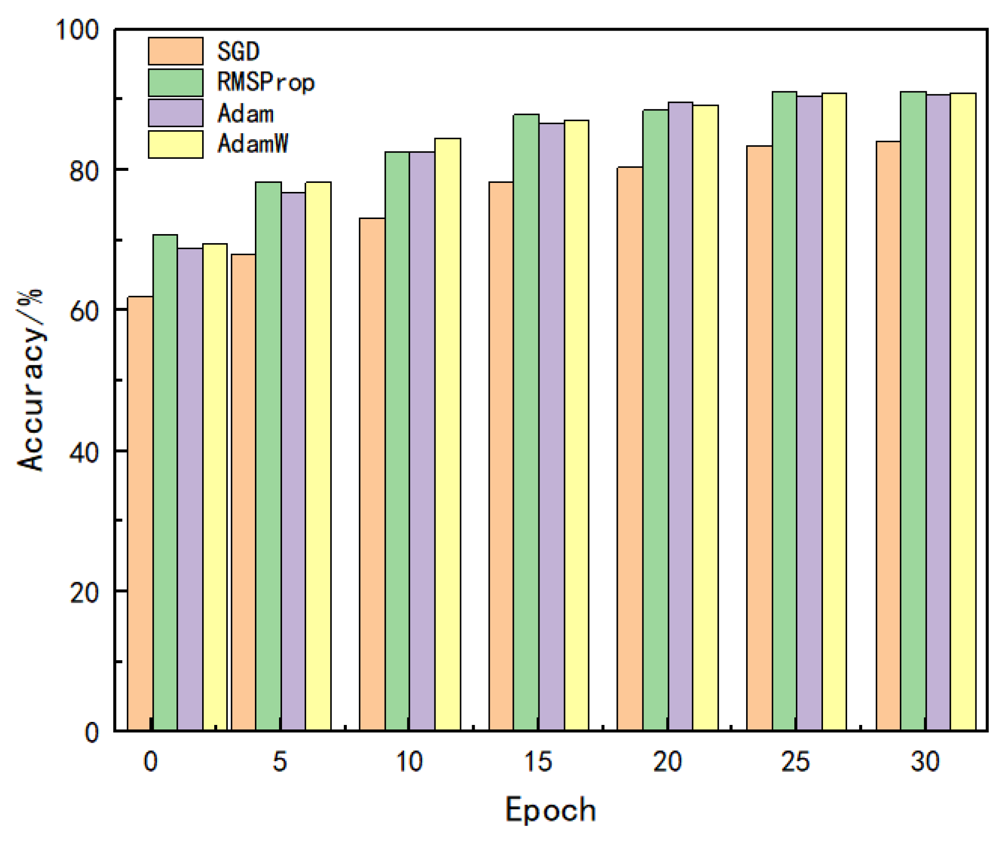
To evaluate the overall effectiveness of different optimization algorithms in terms of training convergence speed, accuracy performance, and loss control, four mainstream optimizers—SGD, RMSProp, Adam, and AdamW—were selected for comparative experiments. All experiments were conducted under the same network architecture, dataset split, and number of training epochs (30 in total). Only the optimizer parameter was varied, while other hyperparameters remained constant to ensure a fair comparison. Figure 7 presents a bar chart comparing the final accuracy achieved by each optimizer. RMSProp achieved the best result at 91.2%, followed by AdamW and Adam, while SGD yielded the lowest accuracy. Overall, both RMSProp and AdamW showed faster convergence in the early training stages, with steadily improving accuracy and consistently better performance. In contrast, SGD converged more slowly and exhibited larger accuracy fluctuations, resulting in suboptimal final performance. For loss comparison, Figure 8 illustrates the training loss curves of each optimizer, with values recorded every five epochs. It can be observed that RMSProp and AdamW achieved faster loss reduction and demonstrated greater stability in the later stages, ultimately converging to lower loss levels. SGD, on the other hand, experienced larger fluctuations during training and struggled to reduce loss effectively, indicating poorer convergence.
These results suggest that RMSProp exhibits a well-balanced advantage across all three dimensions. Therefore, RMSProp was selected as the default optimization strategy in the final model implementation.

3.2.2. Comparative Analysis of Structural Improvements

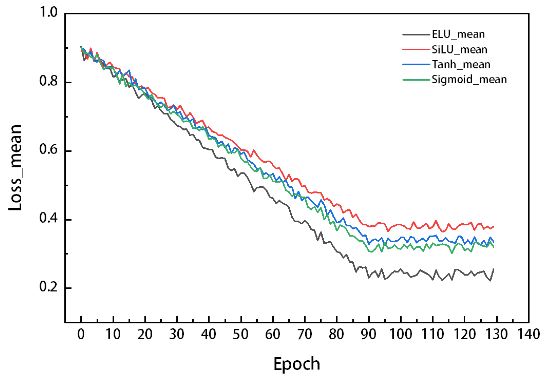
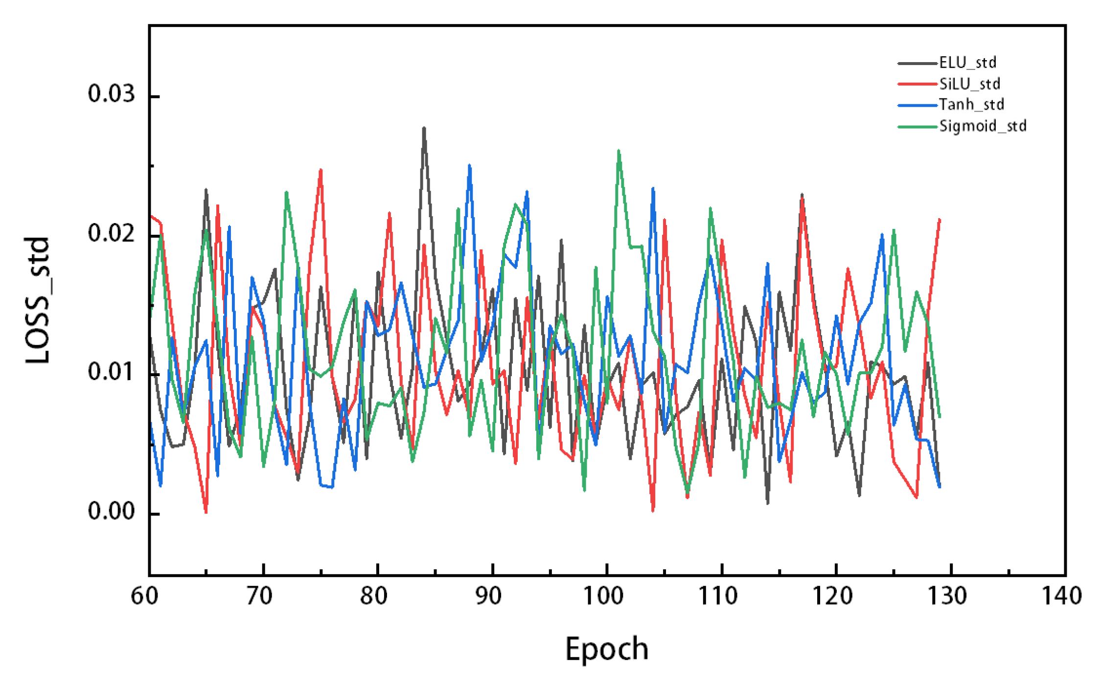
To verify the impact of different activation functions on model performance, four representative functions—ELU, SiLU, Tanh, and Sigmoid—were selected. Under identical model architecture and training parameter settings, three independent experiments were conducted for each function. In addition to focusing on the average loss value, this section also introduces the standard deviation (SD) as a supplementary metric. While the average loss value reflects the overall prediction error across all test samples, relying on this metric alone may not provide a comprehensive assessment of model stability, especially when the loss varies significantly. The standard deviation quantifies the dispersion of the loss values and helps evaluate the consistency of model performance across different samples. A high standard deviation may indicate that the model performs unevenly across the dataset, potentially signaling a risk of overfitting. Therefore, by jointly considering both the average loss and standard deviation, we can more comprehensively assess the model’s accuracy and stability. Figure 9 and Figure 10 show the variation of average loss and corresponding standard deviation intervals across 130 training epochs for each activation function. The results reveal that the ELU activation function outperformed the other three in both convergence speed and final loss value. In the early training stages, the ELU-based model exhibited a faster decline in loss, entering convergence earlier. In the later stages, the loss curve stabilized at a relatively low level, with a final average loss of 0.24 and a standard deviation of approximately 0.015, indicating good robustness and consistency. In contrast, SiLU, Tanh, and Sigmoid showed slightly slower convergence, with final loss values stabilizing at 0.38, 0.34, and 0.32, respectively, and greater fluctuations compared to ELU. Although these functions also showed a degree of stability in later training stages, they were slightly inferior in both loss reduction and convergence quality. Results from multiple experimental rounds confirm that the superior performance of ELU is statistically consistent and not accidental. This may be attributed to ELU’s ability to maintain a non-zero derivative for negative inputs, which alleviates the vanishing gradient problem while retaining the sparsity advantage of ReLU, thus making the model easier to optimize.
In addition, a series of structural improvement strategies were implemented—such as activation function replacement, enhanced regularization, and the addition of a fully connected layer—to construct multiple model variants for comparison. The results demonstrated that each structural enhancement contributed to varying degrees of performance improvement. In particular, the combination of the ELU activation function and L2 regularization significantly improved training stability and final accuracy. Furthermore, to thoroughly compare the effects of different activation functions on model performance, a targeted experiment was designed to evaluate the recognition accuracy, loss, and training time across ELU, SiLU, Tanh, and Sigmoid. The results show that ELU outperformed all other activation functions across all metrics, demonstrating stronger nonlinear feature modeling capability and training efficiency, thus validating its suitability for this application scenario (see Table 2).

3.2.3. Model Performance Comparison

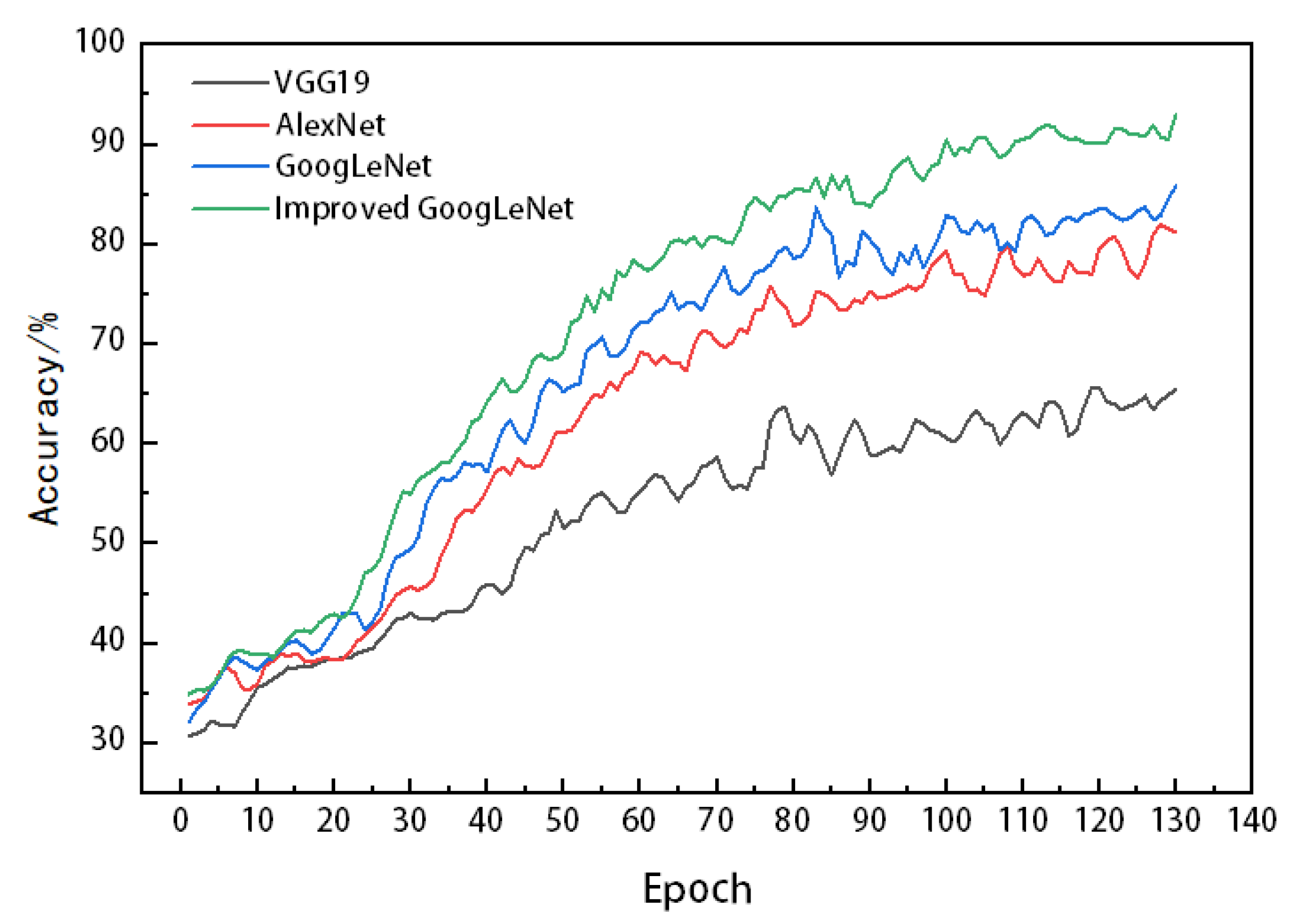
As shown in Table 3, this experiment evaluated the performance of four deep learning models—VGG19, AlexNet, GoogLeNet, and GoogLeNet+RMSProp—on the task of shrimp freshness classification. Their feasibility was analyzed by comparing accuracy, loss, and training time. According to the results, VGG19 achieved the lowest accuracy at only 65.5%. AlexNet improved the accuracy to 81.2%, while GoogLeNet further enhanced it to 85.9%. Among all models, GoogLeNet+RMSProp achieved the best performance with an accuracy of 93%, benefiting from deeper feature extraction and the efficient RMSProp optimization algorithm. This indicates that the model is more capable of capturing freshness features and improving classification performance. In terms of loss, both VGG19 and AlexNet reached a loss value of 0.8, while GoogLeNet reduced it to 0.4. GoogLeNet+RMSProp further decreased the loss to 0.2, demonstrating stronger prediction stability. Regarding training time, VGG19 required the longest time at 46.8 s. Due to its shallower architecture, AlexNet completed training in just 15.5 s. GoogLeNet balanced accuracy and training efficiency with a training time of 27.3 s, while GoogLeNet+RMSProp further improved training efficiency, reducing the training time to 22.1 s and showing higher computational efficiency.
As illustrated in Figure 11, the improved GoogLeNet model demonstrated the best overall performance in the shrimp freshness classification experiment. It achieved high accuracy while effectively reducing the loss value and improving training efficiency. Compared with other models, this method exhibited stronger competitiveness in terms of classification accuracy, stability, and computational efficiency, providing an efficient and feasible solution for intelligent shrimp freshness recognition.

3.3. Visualization Analysis

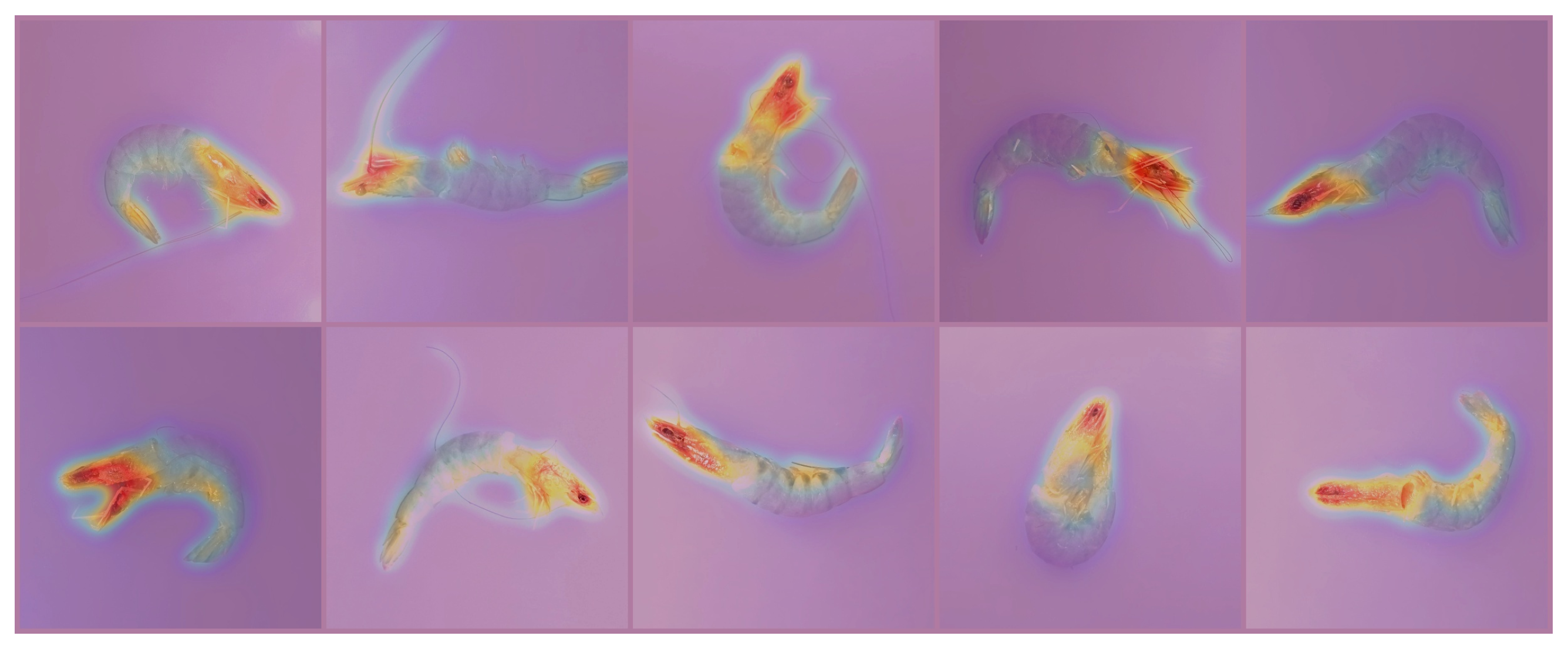
This study selected ten representative images spanning multiple freshness grades and placement orientations. Class-activation maps were computed using Grad-CAM from the terminal convolutional block of the enhanced GoogLeNet (Figure 12). The resulting saliency patterns are largely pose-invariant: the network consistently attends to the abdominal segments, which dominate the grading decision. When abdominal cues are weak or partially occluded, attention shifts to the cephalothorax to provide complementary evidence. These patterns are consistent with the TVB-N–based labels and indicate that the model leverages biologically meaningful features rather than pose or background artifacts, thereby supporting the effectiveness and interpretability of the approach for multi-level shrimp freshness assessment.

4. Conclusions

To meet the need for fast and objective decision-making on shrimp processing lines and to address robustness and generalization challenges arising from inter-sample variability, this study proposes a non-destructive, image-driven freshness assessment method based on an enhanced GoogLeNet. By establishing a labeling scheme aligned with TVB–N and combining data augmentation, architectural refinements, and training-strategy optimization, a complete evaluation pipeline was formed. On the curated shrimp image dataset, the method achieved a test accuracy of 93 % with a test loss of 0.2 ; all improvements over the baselines were statistically significant at the α = 0.05 level (paired t-test; Wilcoxon signed-rank when normality was violated) and were consistent across five independent runs. Qualitative Grad-CAM visualizations further showed pose-invariant attention concentrated on abdominal segments with complementary cues from the cephalothorax, supporting the biological plausibility and interpretability of the model’s decisions and indicating practical potential for in-line screening and process monitoring.
The main contributions of this study include:
  • Constructing a four-category shrimp freshness image dataset rigorously aligned with TVB–N physicochemical indicators, enhancing label reliability and validating the feasibility of image-based non-destructive freshness assessment.
  • Proposing an enhanced GoogLeNet model tailored for small-sample learning, incorporating ELU activation, strengthened L2 regularization, an additional fully connected layer, and the RMSProp optimizer, thereby improving sensitivity to subtle features under limited data.
  • Introducing a multi-dimensional evaluation framework that systematically validates the effectiveness of model improvements through comprehensive performance metrics and visualization tools.
  • Experimentally demonstrating superiority over traditional CNN baselines in convergence speed, robustness, and classification accuracy, showing potential for application in online sorting and real-time monitoring.
  • Providing mechanism-oriented interpretability evidence: Grad-CAM visualizations reveal pose-invariant attention concentrated on abdominal segments with complementary cues from the cephalothorax, indicating biologically meaningful decision features rather than orientation or background artifacts and supporting robustness for in-line deployment.
Despite the promising results, this study has limitations. The shrimp samples were sourced from a single origin and collected under strictly controlled environmental conditions, which may restrict generalizability to other sources, storage conditions, or aquatic species. Moreover, variations in lighting and equipment in real industrial settings were not considered in the current study. Future work will focus on expanding the dataset to include multiple sources, species, and complex environments; exploring lightweight network architectures and embedded deployment for real-time edge scenarios; validating the system on actual processing lines to facilitate translation from laboratory to industry; and investigating multi-modal freshness models (e.g., near-infrared imaging, odor sensors) to enhance reliability and applicability.

Author Contributions

D.H.: Data curation, Writing—original draft. C.Z.: Conceptualization, Methodology, Supervision, Writing—review & editing. R.W.: Investigation, Visualization. Q.Q.: Software, Validation. L.G.: Formal analysis. J.L.: Formal analysis. R.L.: Resources, Project administration. All authors have read and agreed to the published version of the manuscript.

Funding

This work was supported by the Fundamental Research Funds for Zhejiang Provincial Universities and Research Institutes (Grant No. 2021J009), and the Science and Technology Projects of Zhoushan Science and Technology Bureau (Grant Nos. 2011C21001 and 2023C41016).

Institutional Review Board Statement

Fresh marine shrimp were used in this study. Fresh marine shrimp purchased from Zhoushan Seafood Market (Zhoushan, China) were kindly provided by Dr. Cunxi Zhang (Zhejiang Ocean University, Zhoushan, China).

Data Availability Statement

The data presented in this study are available on request from the corresponding author.

Conflicts of Interest

Author Rongsheng Lin was employed by the company Jurong Energy (Xinjiang) Co., Ltd. The remaining authors declare that the research was conducted in the absence of any commercial or financial relationships that could be construed as a potential conflict of interest.

References

  1. Bhatti, M.B.; Sherzada, S.; Ahmad, S.; Qazi, M.A.; Ayub, A.; Khan, S.A.; Khan, M.J.; Rani, I.; Hussain, N.; Nowosad, J.; et al. Comparative Nutritional Profiling of Economically Important Shrimp Species in Pakistan. J. Mar. Sci. Eng. 2025, 13, 157. [Google Scholar] [CrossRef]
  2. Barrow, C.J.; Yamaguchi, K.; Lee, K.; Nishina, S.; Wada, S. High Yields of Shrimp Oil Rich in Omega-3 and Natural Astaxanthin from Pink Shrimp Processing By-Products. ACS Omega 2020, 5, 4864–4873. [Google Scholar] [CrossRef]
  3. Das, S.; Mishra, S. A comprehensive review of the spoilage of shrimp and advances in various indicators/sensors for shrimp spoilage monitoring. Food Control 2023, 145, 109456. [Google Scholar] [CrossRef]
  4. Zhou, Q.; Liu, Y.; Wang, L.; Li, X.; Zhang, M.; Chen, H. Characterization of endogenous enzymes in sword prawn (Parapenaeopsis hardwickii) and their impact on muscle quality during storage. Food Chem. 2023, 405, 134743. [Google Scholar] [CrossRef]
  5. Fan, Y.; Odabasi, A.; Sims, C.A.; Schneider, K.R.; Gao, Z.; Sarnoski, P.J. Determination of aquacultured whiteleg shrimp (Litopenaeus vannamei) quality using a sensory method with chemical standard references. J. Sci. Food Agric. 2021, 101, 5236–5244. [Google Scholar] [CrossRef]
  6. Kim, S.-H.; Jung, E.-J.; Hong, D.-L.; Lee, S.-E.; Lee, Y.-B.; Cho, S.-M.; Kim, S.-B. Quality assessment and acceptability of whiteleg shrimp (Litopenaeus vannamei) using biochemical parameters. Fish. Aquat. Sci. 2020, 23, 21. [Google Scholar] [CrossRef]
  7. Yildiz, M.B.; Yasin, E.T.; Koklu, M. Fisheye freshness detection using common deep learning algorithms and machine learning methods with a developed mobile application. Eur. Food Res. Technol. 2024, 250, 1919–1932. [Google Scholar] [CrossRef]
  8. Banwari, A.; Joshi, R.C.; Sengar, N.; Dutta, M.K. Computer vision technique for freshness estimation from segmented eye of fish image. Ecol. Inform. 2022, 69, 101602. [Google Scholar] [CrossRef]
  9. Cheng, J.H.; Sun, D.W. Recent Applications of Machine Vision in Fish Quality Assessment: A Review. Compr. Rev. Food Sci. Food Saf. 2016, 15, 730–747. [Google Scholar] [CrossRef]
  10. Mjahad, A.; Polo-Aguado, A.; Llorens-Serrano, L.; Rosado-Muñoz, A. Optimizing Image Feature Extraction with Convolutional Neural Networks for Chicken Meat Detection Applications. Appl. Sci. 2025, 15, 733. [Google Scholar] [CrossRef]
  11. Prema, K.; Visumathi, J. Hybrid Approach of CNN and SVM for Shrimp Freshness Diagnosis in Aquaculture Monitoring System using IoT Based Learning Support System. Int. J. Electr. Electron. Res. 2022, 11, 801–805. [Google Scholar] [CrossRef]
  12. Shorten, C.; Khoshgoftaar, T.M. A survey on image data augmentation for deep learning. J. Big Data 2019, 6, 60. [Google Scholar] [CrossRef]
  13. Tang, C.X.; Li, E.B.; Zhao, C.Z.; Li, C. Monitoring the Change Process of Banana Freshness by GoogLeNet. IEEE Access 2020, 8, 223890–223899. [Google Scholar] [CrossRef]
  14. Moncera, C.J.A.; Portillano, G.M.; Agduma, J.T.; Dionson, M.G.D.; Bibangco, E.P. Enhancing Fish Freshness Assessment for Sustainable Fisheries: A Deep Learning Approach with MobileNetV1. Philipp. J. Sci. Eng. Technol. 2024, 1, 10–17. [Google Scholar] [CrossRef]
  15. Shao, Y.; Shi, Y.; Wang, K.; Li, F.; Zhou, G.; Xuan, G. Detection of small yellow croaker freshness by hyperspectral imaging. J. Food Compos. Anal. 2023, 115, 104980. [Google Scholar] [CrossRef]
  16. Tsagkatakis, G.; Nikolidakis, S.; Petra, E.; Kapantagakis, A.; Grigorakis, K.; Katselis, G.; Vlahos, N.; Tsakalides, P. Fish Freshness Estimation through Analysis of Multispectral Images with Convolutional Neural Networks. Electron. Imaging 2020, 2020, 171-1–171-5. [Google Scholar] [CrossRef]
  17. Ye, R.; Chen, Y.; Guo, Y.; Duan, Q.; Li, D.; Liu, C. NIR Hyperspectral Imaging Technology Combined with Multivariate Methods to Identify Shrimp Freshness. Appl. Sci. 2020, 10, 5498. [Google Scholar] [CrossRef]
  18. Huang, W.; Zhao, Z.; Sun, L.; Ju, M. Dual-Branch Attention-Assisted CNN for Hyperspectral Image Classification. Remote Sens. 2022, 14, 6158. [Google Scholar] [CrossRef]
  19. Choompol, A.; Gonwirat, S.; Wichapa, N.; Sriburum, A.; Thitapars, S.; Yarnguy, T.; Thongmual, N.; Warorot, W.; Charoenjit, K.; Sangmuenmao, R. Evaluating Optimal Deep Learning Models for Freshness Assessment of Silver Barb Through Technique for Order Preference by Similarity to Ideal Solution with Linear Programming. Computers 2025, 14, 105. [Google Scholar] [CrossRef]
  20. Li, D.; Bai, L.; Wang, R.; Ying, S. Research Progress of Machine Learning in Extending and Regulating the Shelf Life of Fruits and Vegetables. Foods 2024, 13, 3025. [Google Scholar] [CrossRef] [PubMed]
  21. Cao, X.; Zhang, X.; Chen, W.; Liu, T. Hybrid modeling for fish freshness evaluation using image and physicochemical fusion based on deep learning and regression ensemble. J. Food Eng. 2023, 352, 111488. [Google Scholar] [CrossRef]
  22. Moosavi-Nasab, M.; Khoshnoudi-Nia, S.; Azimifar, Z.; Khademi, B.; Nejati-Farashah, H.; Jafari, H.; Mohammadi-Dehcheshmeh, M. Evaluation of the total volatile basic nitrogen (TVB-N) content in fish fillets using hyperspectral imaging coupled with deep learning neural network and meta-analysis. Sci. Rep. 2021, 11, 5094. [Google Scholar] [CrossRef]
  23. Zhang, Y.; Wei, C.; Zhong, Y.; Wang, H.; Luo, H.; Weng, Z. Deep learning detection of shrimp freshness via smartphone pictures. J. Food Meas. Charact. 2022, 16, 2669–2680. [Google Scholar] [CrossRef]
  24. Kim, S.S.; Yun, D.-Y.; Lee, G.; Park, S.-K.; Lim, J.-H.; Choi, J.-H.; Park, K.-J.; Cho, J.-S. Prediction and visualization of total volatile basic nitrogen in yellow croaker (Larimichthys polyactis) using shortwave infrared hyperspectral imaging. Foods 2024, 13, 3228. [Google Scholar] [CrossRef]
  25. He, H.-J.; Wu, D.; Sun, D.-W. Nondestructive spectroscopic and imaging techniques for quality evaluation and assessment of fish and fish products. Crit. Rev. Food Sci. Nutr. 2015, 55, 864–886. [Google Scholar] [CrossRef]
  26. Cheng, J.-H.; Sun, D.-W.; Pu, H.; Zhu, Z. Development of hyperspectral imaging coupled with chemometric analysis to monitor K value for evaluation of chemical spoilage in fish fillets. Food Chem. 2015, 185, 245–253. [Google Scholar] [CrossRef]
  27. Qin, J.; Vasefi, F.; Hellberg, R.S.; Akhbardeh, A.; Isaacs, R.B.; Yilmaz, A.G.; Hwang, C.; Baek, I.; Schmidt, W.F.; Kim, M.S. Detection of fish fillet substitution and mislabeling using multimode hyperspectral imaging techniques. Food Control 2020, 114, 107234. [Google Scholar] [CrossRef]
  28. SC/T 3113–2002; Frozen Shrimp. Aquatic Industry Standard; Ministry of Agriculture of the People’s Republic of China: Beijing, China, 2002. Available online: https://yyj.moa.gov.cn/kjzl/201904/t20190419_6210548.htm (accessed on 16 March 2025).
  29. GB 2733–2015; National Food Safety Standard—Fresh and Frozen Aquatic Products of Animal Origin. National Health and Family Planning Commission of the People’s Republic of China: Bejing, China, 2015. Available online: https://www.nhc.gov.cn/ewebeditor/uploadfile/2016/05/20160504145248971.pdf (accessed on 16 March 2025).
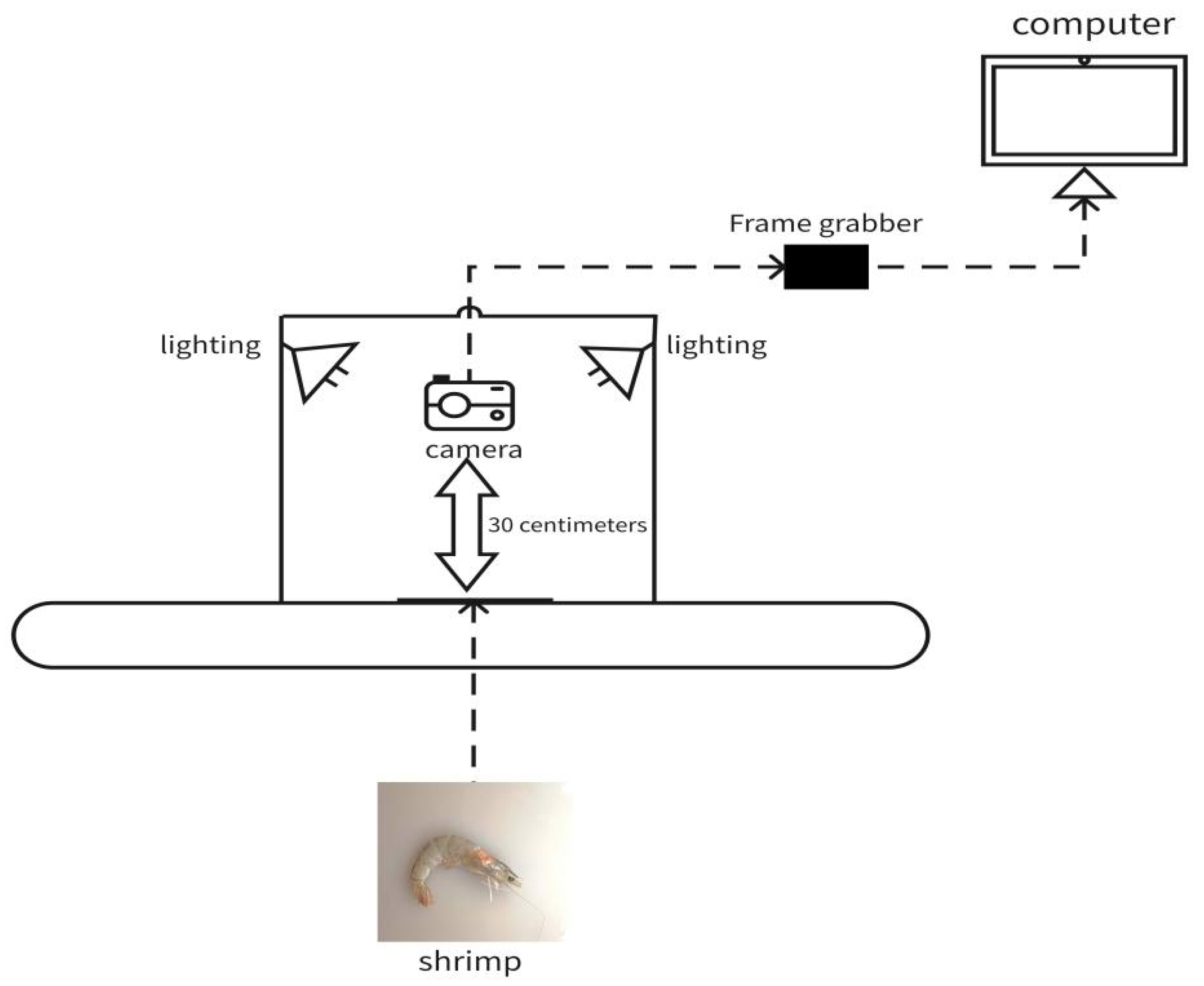
Figure 1. Schematic diagram of image acquisition.
Processes 13 02895 g001
Figure 2. Classification diagram of shrimp products. From left to right: Grade A, Grade B, Qualified, and Non-qualified shrimp products.
Processes 13 02895 g002
Figure 3. Overall research plan.
Processes 13 02895 g003
Figure 4. Inception module.
Processes 13 02895 g004
Figure 5. Architecture of GoogLeNet.
Processes 13 02895 g005
Figure 6. Architecture of the improved GoogLeNet.
Processes 13 02895 g006
Figure 7. Bar chart comparison of accuracy rates among different optimizers per 5 training epochs.
Processes 13 02895 g007
Figure 8. Loss curves of different optimizers per 5 training epochs.
Processes 13 02895 g008
Figure 9. Average loss variation curve.
Processes 13 02895 g009
Figure 10. Standard deviation of loss variation curve.
Processes 13 02895 g010
Figure 11. Accuracy curves of different models.
Processes 13 02895 g011
Figure 12. Thermal diagram. class-activation maps for ten representative samples across different freshness grades and placements. Color scale: warmer colors (red→yellow) denote higher contribution to the predicted class; cooler colors (green→blue) denote lower contribution.
Processes 13 02895 g012
Table 1. Freshness classification sample distribution.
Freshness LevelTraining SetTest SetTotal
First-class20395232616
Second-class11042761380
Qualified14693671836
Non-conforming12393091548
Total585114757380
Table 2. Performance comparison of models with different activation functions.
Activation FunctionAccuracy (%)LossTraining Time (s)
ELU93.00.2022.1
SiLU84.70.4022.0
Tanh85.90.3522.8
Sigmoid87.60.3324.6
Table 3. Performance comparison of different deep learning models.
ModelAccuracy (%)LossTraining Time (s)
VGG1965.50.846.8
AlexNet81.20.815.5
GoogLeNet85.90.427.3
Improved GoogLeNet93.00.222.1
Disclaimer/Publisher’s Note: The statements, opinions and data contained in all publications are solely those of the individual author(s) and contributor(s) and not of MDPI and/or the editor(s). MDPI and/or the editor(s) disclaim responsibility for any injury to people or property resulting from any ideas, methods, instructions or products referred to in the content.