Article

A Dual-Norm Support Vector Machine: Integrating L1 and L Slack Penalties for Robust and Sparse Classification

School of Automation Engineering, Moutai Institute, Renhuai 564507, China
*
Author to whom correspondence should be addressed.
Processes 2025, 13(9), 2858; https://doi.org/10.3390/pr13092858
Submission received: 30 July 2025 / Revised: 30 August 2025 / Accepted: 4 September 2025 / Published: 6 September 2025

Abstract

This paper presents a novel support vector machine (SVM) classification approach that simultaneously accounts for both overall and extreme misclassification errors via a dual-norm regularization strategy. Traditional SVMs minimize the L 1 -norm of slack variables to control global misclassification, while least squares SVM (LSSVM) minimizes the sum of squared errors. In contrast, our method preserves the classical L 1 -norm penalty to maintain overall classification fidelity and incorporates an additional L -norm term to penalize the largest slack variable, thereby constraining the worst-case margin violation. This composite objective yields a more robust and generalizable classifier, particularly effective when occasional large deviations disproportionately affect decision boundaries. The resulting optimization problem minimizes a regularized objective combining the model norm, the sum of slack variables, and the maximum slack variable, with two hyperparameters, C 1 and C 2 , balancing global error against extremal robustness. By formulating the problem under convex constraints, the optimization remains tractable and guarantees a globally optimal solution. Experimental evaluations on benchmark datasets demonstrate that the proposed method achieves comparable or superior classification accuracy while reducing the impact of outliers and maintaining a sparse model structure. These results underscore the advantage of jointly enforcing L 1 and L penalties, providing an effective mechanism to balance average performance with worst-case error sensitivity in support vector classification.

1. Introduction

Support vector machines (SVMs) have long been recognized as one of the most powerful and widely used tools in supervised classification tasks due to their solid theoretical foundations, generalization ability, and effectiveness in high-dimensional spaces [1,2,3]. Traditional SVMs operate by maximizing the margin between data classes while minimizing a regularization term and a slack penalty, often using the L 1 -norm of slack variables to control misclassification [4,5]. Despite their success, conventional SVMs often suffer from high computational complexity and sensitivity to outliers, especially when the misclassification errors exhibit large variance. Despite their remarkable success across a broad spectrum of classification tasks, conventional SVMs are not without notable limitations. In particular, they tend to incur substantial computational costs when applied to large-scale datasets and exhibit heightened sensitivity to outliers or mislabeled instances—especially in scenarios where the misclassification errors show large variance [6,7,8,9,10]. The aforementioned issues have spurred considerable research efforts aimed at improving the computational efficiency, robustness, and generalization capability of SVM-based models. One prominent line of work has focused on robust loss functions, such as Huber loss, ramp loss, or truncated hinge loss, which reduce sensitivity to noise and outliers by down-weighting the influence of misclassified samples with large residuals [8,9,10]. Another important direction involves sparse SVM formulations, particularly those that incorporate L 1 -norm regularization to induce sparsity in support vectors or model parameters, thus improving interpretability and reducing computational costs [11,12]. In parallel, researchers have explored extensions of SVM within the least squares framework (LSSVM) to simplify the optimization by converting the quadratic programming problem into a set of linear equations and alleviate the computational burden and improve training efficiency [13,14]. However, standard LSSVM sacrifices sparsity and inherits a lack of robustness to outliers due to its reliance on a quadratic loss function. To address data uncertainty and distribution shifts in real-world applications, distributionally robust optimization (DRO) has been integrated into support vector machines, significantly enhancing their reliability. For instance, ref. [15] proposed a distributionally robust joint chance-constrained SVM that handles uncertainties by enforcing probabilistic constraints across multiple data scenarios, offering a unified framework for robust classification under ambiguous distributions. Similarly, ref. [16] developed both robust and distributionally robust optimization models specifically for linear SVMs, demonstrating improved generalization and stability by optimizing against the worst-case distribution within an uncertainty set. Extending these ideas to nonlinear classification, ref. [17] introduced a kernel-based distributionally robust chance-constrained SVM that preserves the flexibility of feature mappings while providing probabilistic guarantees on constraint violations. Complementing these methodological advances, ref. [18] presented a scalable chance-constrained SVM framework designed to efficiently learn from large-scale datasets, bridging the gap between computational tractability and theoretical robustness.
These methods have motivated various extensions to enhance the sparsity and robustness of LSSVM. Recent studies have explored non-quadratic loss functions such as Huber loss or ϵ -insensitive loss to mitigate the influence of outliers while retaining smooth optimization properties [19,20]. Additionally, alternative regularization norms beyond the standard L 2 -norm, including L 1 -norm and mixed-norm strategies, have been investigated to encourage sparsity and reduce overfitting [21,22]. To further improve performance, hybrid optimization schemes combining convex–concave procedures, proximal algorithms, or kernel pruning techniques have also been proposed for efficient and adaptive model training [23,24]. Among these developments, combining different norm-based penalties (e.g., L 1 , L ) on slack variables has shown promising potential in simultaneously controlling model complexity and improving classification reliability [25,26]. Also, numerous variants of SVM and LSSVM have been developed to address these issues. Robust SVM formulations aim to limit the influence of outliers by using alternative loss functions or data-driven weighting strategies [27]. Sparse SVM models incorporate L 1 -based regularization or feature selection techniques to achieve compact decision functions [28]. Non-convex or hybrid regularization schemes have also been introduced to balance sparsity and accuracy [29]. In the context of LSSVM, recent advancements include fuzzy-weighted LSSVMs [30], multi-kernel frameworks [31], and adaptive loss modifications to enhance model robustness [32]. Recent advances in robust and sparse support vector machine (SVM) methods have significantly improved the handling of noisy and high-dimensional data. Generalized adaptive Huber-loss twin SVM frameworks [33] dynamically adjust robustness parameters to mitigate the effect of outliers, achieving superior performance in high-noise scenarios. Fast truncated Huber-loss SVM approaches [34] have been developed for large-scale classification, leveraging efficient optimization algorithms to maintain both computational efficiency and high accuracy. Extensions of Huber-loss SVM to multi-task learning frameworks [35] enhance robustness and interpretability when handling multiple related classification tasks simultaneously. Structured sparse SVM models with ordered non-convex penalties [36] effectively ensure model sparsity and interpretability in high-dimensional datasets with ordered covariates. In addition, sparse least-squares Universum twin bounded SVMs [37] integrate classification with feature selection through sparsity-inducing mechanisms, improving robustness against noisy observations while reducing model complexity. Collectively, these developments provide a comprehensive foundation for integrating robustness and sparsity in modern SVM frameworks. In the past five years, the research community has renewed its focus on enhancing SVM models to improve robustness and interpretability, particularly in the face of class imbalance and noisy data. For instance, a capped squared-loss SVM was proposed to reduce the impact of large-margin violations while maintaining computational efficiency in large-scale settings [38]. In the domain of least squares SVMs (LSSVMs), variants using capped-norm distance metrics have been introduced to mitigate noise and enhance robustness under adverse conditions [39,40]. More recently, novel loss functions—such as smoothed or truncated formulations—have been integrated with hybrid regularization to simultaneously achieve sparsity and stability in classification tasks [41,42]. Although these works have collectively advanced the trade-off between accuracy, robustness, and sparsity, most approaches still rely on a single-norm penalty and do not explicitly address both aggregate misclassification and extreme violation in a unified framework. Motivated by the need to construct classifiers that are both accurate and robust to extreme deviations, this work introduces a dual-norm regularization framework for SVMs. By jointly enforcing the L 1 -norm to preserve global classification fidelity and sparsity, and the L -norm to constrain the worst-case margin violation, our approach achieves a balanced trade-off between average performance and extreme-case robustness. This novel formulation advances existing SVM methodologies by explicitly integrating both global and extremal error control within a convex, tractable optimization framework.
The primary contributions of this study are as follows. First, we propose a novel support vector machine formulation that simultaneously incorporates the L 1 -norm and L -norm of the slack variables. The L 1 -norm ensures global classification fidelity and promotes sparsity in the solution, while the L -norm explicitly penalizes the largest individual margin violation, thereby enhancing robustness against extreme outliers. This dual-norm strategy achieves a balanced trade-off between average-case and worst-case performance, a combination not previously explored in the SVM literature. Second, we formulate the dual-norm SVM problem under convex constraints, resulting in a computationally tractable optimization task. The model includes two tunable hyperparameters, C 1 and C 2 , which provide flexible control over the trade-off between minimizing misclassification and enforcing robustness. This formulation guarantees global optimality and can be efficiently solved using standard convex optimization techniques.
The remainder of this paper is organized as follows. Section 2 reviews the background of Support Vector Machine (SVM) and least squares SVM (LSSVM), and outlines the motivation behind our proposed approach. Section 3 introduces the dual-norm support vector classification model. Experimental results and analysis are presented in Section 4. Finally, Section 5 concludes the paper.

2. Preliminaries

2.1. Support Vector Machine (SVM)

Support vector machine (SVM) is a well-established supervised learning algorithm used primarily for binary classification. The key idea behind SVM is to find a hyperplane that maximizes the margin between two linearly separable classes in a given feature space. To handle non-separable data, slack variables are introduced to allow certain samples to violate the margin constraints. This leads to the formulation of the so-called soft-margin SVM, which strikes a trade-off between maximizing the margin and minimizing misclassification. SVMs use the hinge loss to penalize misclassifications. In contrast, least squares SVM (LSSVM) reformulates the problem using equality constraints and a squared loss function, which reduces the optimization to solving a set of linear equations. Due to these differences, standard SVM is preferred when robustness to outliers and sparsity of the solution are critical, as it only relies on support vectors. LSSVM is often favored in large-scale regression or classification tasks where computational efficiency is more important, since solving linear equations is typically faster than quadratic programming.
We consider a binary classification problem with training samples { ( x i , y i ) } i = 1 N , where x i R d denotes the input features and y i { 1 , + 1 } the corresponding class labels. Our objective is to learn a decision function of the form
f ( x ) = w ϕ ( x ) + b ,
where w is the weight vector, b R is the bias term, and ϕ ( · ) denotes a nonlinear mapping to a high-dimensional feature space induced by a kernel function K ( x i , x j ) = ϕ ( x i ) , ϕ ( x j ) .
Mathematically, the primal problem of the soft-margin SVM is formulated as [4,5]:
min w , b , ξ 1 2 w 2 + C i = 1 N ξ i s . t . y i ( w ϕ ( x i ) + b ) 1 ξ i , ξ i 0 , i = 1 , , N
Here, ξ i is a slack variables representing margin violations, and C > 0 is a regularization parameter that controls the trade-off between margin maximization and classification error.
The optimization problem is convex and can be solved efficiently by transforming it into its dual form using Lagrange multipliers and Karush–Kuhn–Tucker (KKT) conditions. The final decision function is expressed in terms of a subset of training samples called support vectors, which lie on or within the margin boundaries.

2.2. Least Squares Support Vector Machine (LSSVM)

SVM and LSSVM are both kernel-based learning algorithms, but they differ in formulation, loss functions, and optimization procedures. Standard SVM aims to find a hyperplane that maximally separates classes by solving a quadratic programming problem with inequality constraints, using the hinge loss to penalize misclassification. This formulation results in a sparse solution that depends only on support vectors, which enhances interpretability and robustness to outliers. However, solving the quadratic programming problem can be computationally intensive for large datasets. LSSVM, in contrast, reformulates the SVM problem by replacing inequality constraints with equality constraints and using a squared loss function. This converts the optimization into a set of linear equations, which can be solved more efficiently, making LSSVM particularly suitable for large-scale problems or real-time applications. The trade-off is that LSSVM typically produces a dense solution, potentially reducing sparsity and sensitivity to outliers compared to standard SVM. In summary, SVM is advantageous when sparsity, robustness to outliers, and interpretability are prioritized, while LSSVM is preferred in scenarios where computational efficiency and scalability are more important. The choice between the two depends on the problem requirements, dataset size, and the desired balance between robustness and efficiency.
Given a training dataset
D = ( x i , y i ) x i R d , y i { 1 , + 1 } , i = 1 , 2 , , N ,
the primal problem of LSSVM for binary classification is formulated as [13,14]
min w , b , ξ 1 2 w 2 + γ 2 i = 1 N ξ i 2 subject to y i w ϕ ( x i ) + b = 1 ξ i , i = 1 , , N ,
where w R d is the weight vector in the feature space, b R is the bias term, ξ = [ ξ 1 , , ξ N ] are the slack variables, γ > 0 is a regularization parameter that controls the trade-off between model complexity and training error.
The corresponding Lagrangian for the optimization problem is
L ( w , b , ξ , α ) = 1 2 w 2 + γ 2 i = 1 N ξ i 2 i = 1 N α i y i ( w ϕ ( x i ) + b ) ( 1 ξ i ) ,
where α i are Lagrange multipliers. By applying the Karush–Kuhn–Tucker (KKT) conditions, the optimization can be reduced to solving the following linear system:
0 y y Ω + 1 γ I b α = 0 1 ,
where y = [ y 1 , , y N ] , Ω i j = y i y j K ( x i , x j ) with kernel K ( x i , x j ) = ϕ ( x i ) ϕ ( x j ) , and I is the identity matrix.
The final decision function is given by
f ( x ) = i = 1 N α i y i K ( x i , x ) + b .
Compared to standard SVMs, LSSVMs offer a significant computational advantage by transforming the original quadratic programming problem into a set of linear equations. This simplification makes LSSVM particularly appealing for large-scale problems and real-time applications. However, despite its efficiency, LSSVM suffers from two notable limitations:
(1)
Lack of sparsity: Unlike classical SVMs, where only a subset of support vectors contributes to the decision function, LSSVM typically results in dense solutions because all training samples are involved in the final model. This not only increases storage and evaluation cost but also reduces model interpretability.
(2)
Sensitivity to outliers: The use of squared error loss on slack variables can overly penalize large deviations, making the model less robust to noisy data or outliers.
These drawbacks have motivated various extensions to enhance the sparsity and robustness of LSSVM. Recent studies have explored non-quadratic loss functions, alternative regularization norms, and hybrid optimization schemes to address these issues. Among them, combining different norm-based penalties (e.g., L 1 , L ) on slack variables has shown promising potential in simultaneously controlling model complexity and improving classification reliability.

2.3. Motivation for Dual-Norm Regularization

Both SVM and LSSVM focus on aggregate error minimization: SVM uses the L 1 -norm of slack variables, while LSSVM uses the L 2 -norm. Neither approach explicitly addresses the largest individual slack variable, which can represent the most severe margin violation. However, in critical applications where worst-case misclassification must be controlled, the L -norm (i.e., the maximum slack variable) becomes an essential component.
This motivates our proposed approach, which incorporates both L 1 - and L -norm regularization into a unified framework. By minimizing the total misclassification and simultaneously constraining the maximum margin violation, our method offers improved robustness and interpretability without sacrificing optimization tractability. The following section presents the detailed formulation of this dual-norm model.

3. Dual-Norm Regularization for Support Vector Classification

3.1. Construction of Support Vector Classification Model Under Dual-Norm Regularization

In the context of support vector classification, various norms are employed to regularize the optimization problem. The L 1 -norm is defined as x 1 = i = 1 n | x i | , where x i represents each element of the vector x . This norm promotes sparsity in solutions, making it particularly useful in scenarios where only a subset of features or samples significantly influences the outcome. The L 2 -norm, given by x 2 = i = 1 n x i 2 , encourages small but non-zero values across all elements, leading to dense solutions. Lastly, the L -norm, expressed as x = max ( | x 1 | , | x 2 | , . . . , | x n | ) , focuses on penalizing the largest absolute value among the elements, thereby controlling the worst-case scenario.
Each norm finds its application based on specific requirements. The L 1 -norm is often used when the goal is to achieve a sparse solution, such as in feature selection. The L 2 -norm is beneficial for problems requiring smoothness and stability, like regression tasks. Meanwhile, the L -norm is advantageous in settings where robustness against extreme outliers is critical. From the perspective of SVM and LSSVM, these norms manifest differently. Traditional SVMs minimize the L 1 -norm of slack variables to control overall misclassification, ensuring that most data points are correctly classified while allowing some flexibility for noisy samples. On the other hand, LSSVM employs the Ł 2 -norm to minimize the sum of squared errors, resulting in a more computationally efficient solution but at the cost of sensitivity to outliers due to the quadratic penalty applied to large deviations. A schematic illustration of the proposed method is shown in Figure 1.
The proposed method integrates both the L 1 -norm and L -norm penalties into the objective function:
minimize : 1 2 w T w + C 1 i = 1 N ξ i + C 2 λ subject to : y i ( w · ϕ ( x i ) + b ) 1 ξ i y i ( w · ϕ ( x i ) + b ) 1 λ ξ i 0 , λ 0
Here, w denotes the weight vector, b is the bias term, ϕ ( · ) maps input features into a higher-dimensional space, ξ i measures individual misclassification errors, and λ controls the maximum margin violation. The optimization problem presented introduces two distinct regularization parameters, C 1 and C 2 , which govern the trade-off between classification accuracy and robustness to extreme margin violations. These hyperparameters play complementary roles in shaping the behavior of the resulting classifier and must be interpreted in the context of the dual-norm regularization strategy employed. The parameter C 1 controls the overall penalty associated with the sum of individual slack variables ξ i , which represent the degree to which each training sample violates the margin constraint. This term is directly analogous to the standard L 1 -norm penalty used in classical support vector machines (SVMs), where a larger C 1 enforces stricter adherence to the margin, thereby reducing the number of misclassified samples at the expense of a potentially less generalizable decision boundary. As such, C 1 primarily influences the global classification fidelity and governs the model’s tolerance to average-case errors.
In contrast, the parameter C 2 regulates the influence of the maximum slack variable λ , which upper bounds the worst-case margin violation across all training samples. By explicitly constraining the extremal deviation, C 2 introduces a form of robustness that is not captured by the aggregate penalty alone. A larger C 2 emphasizes the minimization of the most severe misclassification error, effectively shrinking the influence of outliers or adversarial samples that could otherwise distort the decision boundary. This is particularly valuable in scenarios where a single large deviation may disproportionately affect the model’s performance on unseen data. Together, C 1 and C 2 enable a nuanced control over the balance between average-case accuracy and worst-case robustness. While C 1 ensures that the classifier remains sensitive to the majority of training instances, C 2 safeguards against overfitting to extreme deviations, thereby promoting better generalization. The dual regularization mechanism thus allows for a more adaptive and resilient classification model compared to traditional SVMs or least squares SVMs (LSSVMs), which rely on a single regularization parameter.
Moreover, the convexity of the formulation ensures that the interplay between C 1 and C 2 can be analyzed in a well-defined optimization landscape, where their respective contributions to the objective function can be systematically tuned to achieve the desired performance–robustness trade-off. In practice, the optimal values of C 1 and C 2 are typically determined through cross-validation or other model selection techniques, depending on the specific characteristics of the dataset and the application context.
To solve the above optimization problem, we introduce the Lagrangian function
L = 1 2 w T w + C 1 i = 1 N ξ i + C 2 λ i = 1 N α i y i ( w · ϕ ( x i ) + b ) ( 1 ξ i ) i = 1 N β i y i ( w · ϕ ( x i ) + b ) ( 1 λ ) i = 1 N μ i ξ i ν λ
where α i , β i , μ i , ν 0 are Lagrange multipliers. Taking partial derivatives with respect to w , b, ξ i , and λ , and setting them to zero yields
L w = w i = 1 N ( α i + β i ) y i ϕ ( x i ) = 0 , w = i = 1 N ( α i + β i ) y i ϕ ( x i )
L b = i = 1 N ( α i + β i ) y i = 0 , i = 1 N ( α i + β i ) y i = 0
L ξ i = C 1 α i μ i = 0 , C 1 = α i + μ i
L λ = C 2 i = 1 N β i ν = 0 . C 2 = i = 1 N β i + ν
The Lagrange multipliers μ i and ν satisfy the non-negativity conditions μ i 0 and ν 0 and feasible ranges for α i and β i can be obtained:
0 α i C 1 , 0 i = 1 N β i C 2 ,
which reflect the upper bounds imposed by the corresponding regularization parameters C 1 and C 2 .
Substituting Equations (6)–(9) back into the Equation (5) results in the dual function
W ( α , β ) = i = 1 N ( α i + β i ) 1 2 i = 1 N j = 1 N ( α i + β i ) ( α j + β j ) y i y j K ( x i , x j )
where K ( x i , x j ) = ϕ ( x i ) T ϕ ( x j ) represents the kernel function, which typically includes commonly used types such as the linear kernel, polynomial kernel, radial basis function (RBF) kernel, sigmoid kernel, and cosine similarity kernel. Among these, the radial basis function kernel is selected in this study due to its favorable properties, such as strong nonlinearity and locality [43]. Specifically, the RBF kernel is defined as
K ( x i , x j ) = exp γ x i x j 2 2 ,
where γ > 0 is a kernel hyperparameter that controls the width of the Gaussian function. The dual optimization problem then becomes
minimize : i = 1 N ( α i + β i ) + 1 2 i , j = 1 N ( α i + β i ) ( α j + β j ) y i y j K ( x i , x j ) subject to : i = 1 N ( α i + β i ) y i = 0 0 α i C 1 , i 0 β i , i = 1 N β i C 2
Further, the above optimization problem can be expressed in compact vector-matrix form to facilitate numerical implementation and theoretical analysis.
minimize 1 T ( α + β ) + 1 2 ( α + β ) T K ( α + β )
subject to ( α + β ) T y = 0
0 α C 1 1
β 0 , 1 T β C 2
where y = [ y 1 , y 2 , , y N ] T , α = [ α 1 , α 2 , , α N ] T , Q R N × N the Gram matrix with entries Q i j = y i y j K ( x i , x j ) and β = [ β 1 , β 2 , , β N ] T denote the vectors of Lagrange multipliers corresponding to the L 1 -norm and L -norm constraints, respectively; 1 is an N-dimensional column vector of ones; y = [ y 1 , y 2 , , y N ] T represents the vector of class labels; K R N × N is the kernel matrix with entries K i j = K ( x i , x j ) ; 0 is an N-dimensional column vector of zeros.
This convex quadratic programming problem ensures a globally optimal solution and computational tractability. Furthermore, the proposed method inherits the sparsity property from classical SVMs. Specifically, only those samples with non-zero α i or β i contribute to the final decision function:
f ( x ) = i = 1 N ( α i + β i ) y i K ( x i , x ) + b
Thus, the model remains sparse, with only a subset of training samples—those either misclassified or contributing to the worst-case margin violation—affecting the decision boundary. This characteristic, combined with the robustness provided by the L -norm constraint, makes the proposed method highly effective in scenarios where occasional large deviations can disproportionately impact decision boundaries. Through careful tuning of hyperparameters C 1 and C 2 , one can achieve a balanced performance between average-case accuracy and worst-case robustness, offering an improved mechanism for support vector classification under challenging conditions.
The incorporation of the L 1 -norm and L -norm into the regularization strategy provides a powerful tool for mitigating the influence of outliers while preserving model sparsity. By enforcing these penalties simultaneously, the proposed approach addresses limitations inherent in traditional SVM formulations, delivering enhanced robustness and interpretability. These properties make it especially suitable for applications where reliability and resistance to extreme deviations are paramount, such as financial risk assessment, medical diagnosis, and autonomous systems.
Moreover, the theoretical foundation of the proposed method guarantees that the optimization problem remains convex, ensuring that any local optimum found is indeed a global one. This aspect is crucial for practical implementation, as it allows for efficient and reliable computation of the classifier parameters. Experimental evaluations on benchmark datasets further validate the effectiveness of the proposed technique, demonstrating its ability to achieve comparable or superior classification accuracy compared to conventional methods while effectively reducing the impact of outliers and maintaining a sparse model structure.
The proposed dual-norm regularized SVM framework presented here offers significant improvements over existing techniques by combining the benefits of both L 1 and L norms. It achieves a delicate balance between minimizing overall misclassification errors and controlling worst-case deviations, providing a versatile and robust classification tool tailored for modern machine learning challenges. Through rigorous mathematical derivation and empirical validation, this work highlights the potential of integrating multiple regularization strategies to enhance the performance and applicability of support vector machines.

3.2. Hyperparameter Roles, Interaction, and Selection Strategy

The proposed optimization problem introduces two hyperparameters, C 1 and C 2 , formulated as Equation (4), as shown in Table 1, which provides a concise summary of their distinct roles in our method.
The two hyperparameters serve complementary but distinct functions:
(1)
The term C 1 i = 1 N ξ i penalizes individual slack variables ξ i , thereby controlling sample-level accuracy. A larger C 1 enforces stricter adherence to the training samples, which may reduce misclassification but increase the risk of overfitting.
(2)
The term C 2 λ penalizes the global slack variable λ , thereby regulating global sparsity and robustness. Increasing C 2 enforces tighter margin consistency across all samples, resulting in sparser solutions that are less sensitive to noise. Thus, C 1 emphasizes local accuracy, whereas C 2 emphasizes global structure and robustness. The performance of the optimization model depends on the relative magnitudes of C 1 and C 2 :
(1)
When C 1 C 2 , the model behaves similarly to a standard SVM, focusing primarily on minimizing sample-level errors.
(2)
When C 2 C 1 , the optimization emphasizes global sparsity, producing more compact models that are robust to outliers, albeit at the potential cost of reduced accuracy.
(3)
A balanced configuration achieves a trade-off between classification accuracy and sparsity, which is the central motivation for introducing both hyperparameters.
To ensure reproducibility and fair comparison with baseline methods, the following procedure is adopted for hyperparameter selection:
(1)
Hyperparameter Search Strategy: The hyperparameters C 1 and C 2 are optimized using a two-stage grid search procedure consisting of coarse tuning and fine tuning. In the coarse tuning stage, both C 1 and C 2 are explored over a wide logarithmic grid:
C 1 , C 2 { 10 3 , 10 2 , 10 1 , 10 0 , 10 1 , 10 2 , 10 3 } .
This stage aims to roughly identify the region in which the optimal hyperparameters lie. For instance, if the best performance during coarse tuning is observed at C 1 = 10 2 and C 2 = 10 1 , the fine-tuning stage further refines the search within a narrower range centered around these values. Specifically, the fine-tuning grid is constructed as
C 1 [ 10 1.5 , 10 2.5 ] , C 2 [ 10 0.5 , 10 1.5 ] ,
with smaller incremental steps on the logarithmic scale, such as 0.1 in the exponent. This hierarchical strategy ensures that the search process is computationally efficient while maintaining a high likelihood of locating the optimal hyperparameters.
(2)
Cross-Validation: A grid search with 5-fold cross-validation is applied to jointly optimize ( C 1 , C 2 ) .
(3)
Selection Criterion: The optimal pair is determined by a composite evaluation index:
J ( C 1 , C 2 ) = α · Accuracy ( 1 α ) · SV_ratio , α [ 0 , 1 ] ,
where SV_ratio denotes the proportion of support vectors. Unless otherwise specified, we set α = 0.5 to balance accuracy and sparsity.
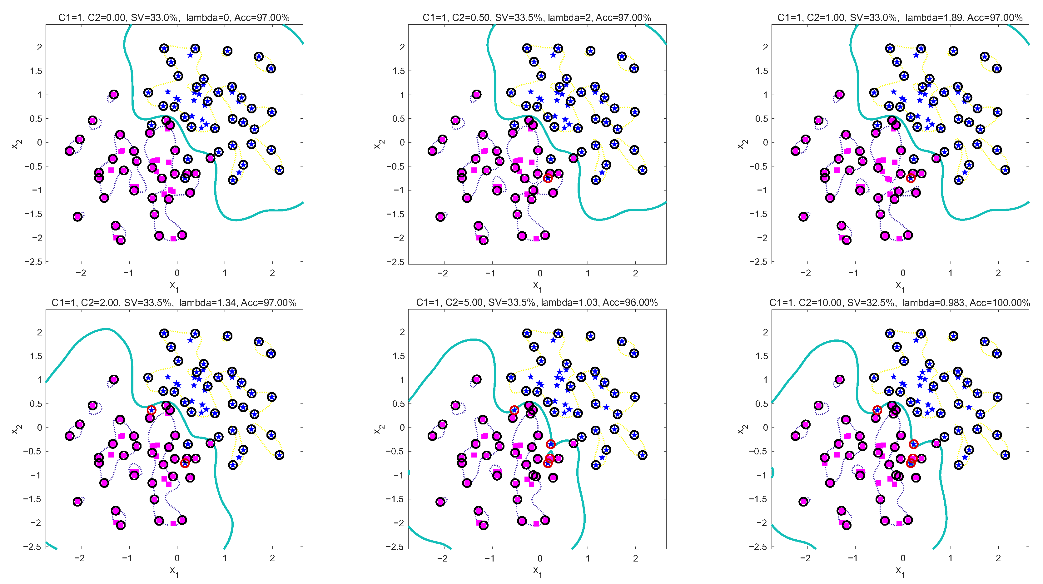
Next, two classification datasets are generated using two random functions (X = [randn(N,2) + 1; randn(N,2) − 1] generated in MATLAB2025a) to provide a preliminary analysis of the roles of the two hyperparameters, C 1 and C 2 , in the proposed method, where identifying data points located on or near the classification boundary poses certain challenges. When C 1 is fixed and C 2 is varied, the classification accuracy and sparsity characteristics are shown in Figure 2, and Table 2 presents a comparison of performance metrics with varying C 2 .
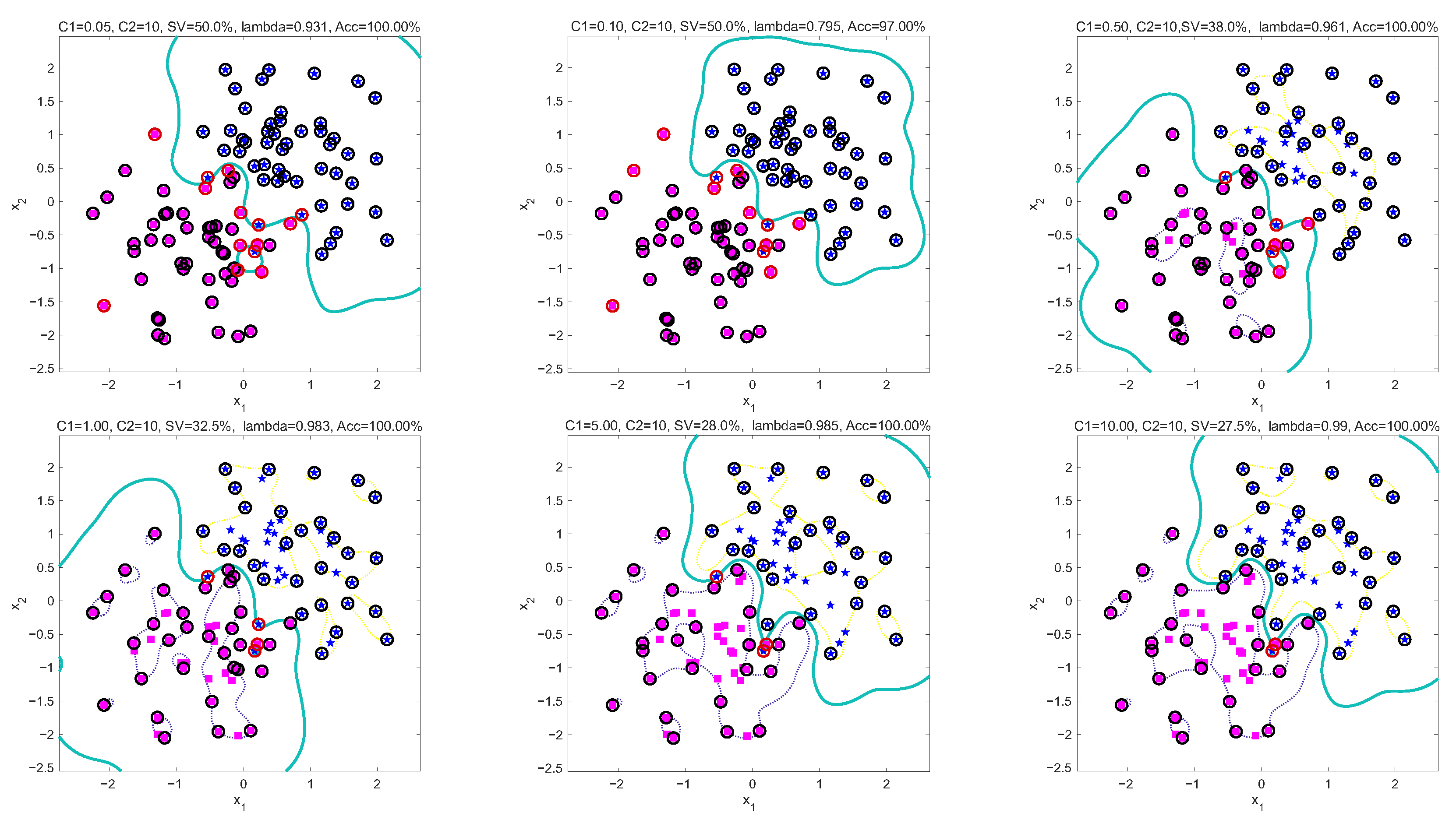
When C 2 is fixed and C 1 is increased, Figure 3 illustrates the classification accuracy and sparsity characteristics, which are further summarized in Table 2.
For example, when C 1 is fixed at 10, varying C 2 from 0 to 10 shows that the support vector ratio gradually decreases from 0.56 to 0.55, indicating that the model becomes slightly sparser as the influence of the global slack regularization increases. The sum of β values rises with C 2 , reflecting stronger activation of the λ -related constraints, while the median λ remains close to 0.99, suggesting consistent enforcement of the upper-bound constraint. Across all C 2 values, both training and test accuracies remain high (≥97%), demonstrating that the model maintains robust classification performance even under increasing global slack penalties. Overall, the results highlight that, with a large C 1 , the model effectively balances sparsity, constraint enforcement, and predictive accuracy as C 2 varies.

3.3. Sparsity Analysis Under Dual-Norm Regularization

This formulation differs from the standard soft-margin SVM only by introducing a single additional global slack variable λ with a linear penalty term C 2 · λ . As a result, we have the following characteristics:
(1)
The primal problem remains a convex quadratic program (QP) with d + N + 2 variables (d: feature dimension; N: number of samples, 1; additional variables: λ ).
(2)
The dual problem introduces an additional dual variable corresponding to λ , but the kernelized QP structure remains intact.
(3)
The complexity of solving the dual remains O ( N 3 ) in the worst case for standard QP solvers, similar to standard SVM, because the Hessian structure is still dominated by the N × N kernel matrix.
(4)
The only overhead is one additional constraint and one additional variable, which is negligible compared to the N slack variables already present in classical SVM.
Therefore, the theoretical complexity remains asymptotically equivalent to that of standard SVM formulations.
To analyze the sparse solutions of the proposed optimization problem, we leverage the Karush–Kuhn–Tucker (KKT) conditions, which characterize the optimality of primal and dual variables. Now, we define the function g i ( · ) as
g i ( · ) = y i w · ϕ ( x i ) + b 1 ξ i 0 ,
and h i ( · ) as
h i ( · ) = y i w · ϕ ( x i ) + b 1 λ 0
The KKT conditions include complementary slackness, which is critical for sparsity analysis: α i g i ( · ) = 0 , β i h i ( · ) = 0 , μ i s i ( · ) = 0 , and ν t ( · ) = 0 , where α i , β i , μ i , ν 0 are dual variables. Below is the classification of sparse solutions based on these conditions:
(1)
Sparse Solutions Induced by L 1 -Norm Slack Variables ( ξ i )
The L 1 -norm penalty on ξ i contributes to sparsity through the relationship α i + μ i = C 1 (derived from Lagrangian derivatives) and complementary slackness μ i ξ i = 0 :
Case 1: α i = 0 Here, μ i = C 1 > 0 , so ξ i = 0 (from μ i ξ i = 0 ). The first constraint becomes y i ( w · ϕ ( x i ) + b ) 1 , meaning the sample x i lies on or within the correct side of the margin. Since α i = 0 , this sample does not contribute to the model parameter w = j = 1 N ( α j + β j ) y j ϕ ( x j ) , making it a non-support vector and enhancing sparsity.
Case 2: 0 < α i < C 1 Here, μ i = C 1 α i > 0 , so ξ i = 0 (from μ i ξ i = 0 ). The first constraint is active: y i ( w · ϕ ( x i ) + b ) = 1 , indicating x i is a support vector lying exactly on the margin. Though α i 0 , such samples are sparse in practice because only margin-boundary samples satisfy this condition.
Case 3: α i = C 1 Here, μ i = 0 , allowing ξ i 0 . The first constraint may be inactive ( y i w · ϕ ( x i ) + b ) < 1 ), meaning x i is a misclassified sample or lies outside the margin. However, α i = C 1 is bounded, and such samples are rare in well-regularized models, preventing dense solutions.
(2)
Sparse Solutions Induced by L -Norm Slack Variable ( λ )
The L -norm penalty on λ contributes to sparsity through i = 1 N β i + ν = C 2 and complementary slackness β i h i ( · ) = 0 :
Case 1: β i = 0 The second constraint y i ( w · ϕ ( x i ) + b ) 1 λ may be inactive or active, but β i = 0 means x i does not contribute to the worst-case margin violation. Such samples do not affect w (since β i = 0 ), reinforcing sparsity.
Case 2: β i > 0 Here, h i ( · ) = 0 (from β i h i ( · ) = 0 ), so y i ( w · ϕ ( x i ) + b ) = 1 λ . This indicates x i is associated with the maximum slack variable λ (i.e., it is a worst-case violator). However, the constraint i = 1 N β i C 2 limits the number of such samples—only a few worst-case violators can have β i > 0 , ensuring sparsity.
(3)
Joint Sparsity from L 1 -Norm and L -Norm Fusion
The combination of L 1 and L penalties amplifies sparsity through Mutual Exclusion of Non-Support Vectors: Samples with both α i = 0 and β i = 0 are completely excluded from w , as they contribute nothing to the model. These samples form the majority in sparse solutions. Bounded Dual Variables: The constraints 0 α i C 1 and i = 1 N β i C 2 prevent excessive non-zero dual variables, ensuring that only critical samples (margin-boundary or worst-case violators) retain non-zero α i or β i .
Consequently, the sparsity in the proposed model is driven by the following complementary mechanisms: the L 1 -norm promotes sparsity in the coefficients α i by forcing them to zero for samples that lie within the margin, effectively excluding them from the support vector set, while the L -norm encourages sparsity in the coefficients β i by assigning non-zero values only to the worst-case margin violators, constrained by the global budget parameter C 2 . Overall, the dual-norm regularization framework induces a two-level sparse solution:
(1)
Local sparsity: arising from the selective activation of α i for margin-violating or support vectors, regulated by the L 1 -norm.
(2)
Extreme-point sparsity: due to the activation of only the most significant margin violator(s) through β i , regulated by the L -like component.
This structured sparsity not only reduces model complexity but also improves interpretability and generalization performance, especially in scenarios involving outliers or imbalanced errors.

3.4. Discussion

The proposed dual-norm SVM framework retains the core principles of large-margin learning, thereby inheriting the generalization guarantees associated with margin-based classifiers. Under the PAC-learning framework, the generalization error of SVMs is primarily governed by the margin and the capacity of the hypothesis space, often quantified through VC-dimension or Rademacher complexity. By introducing an additional L penalty on slack variables, our method explicitly limits the largest margin violation, preventing a single extreme outlier from significantly reducing the effective margin. This modification does not alter the hypothesis space complexity, as the kernel-induced feature mapping remains unchanged; rather, it refines the empirical risk component, making it more robust under heavy-tailed or noisy distributions. Consequently, the dual-norm penalty can be viewed as a regularized risk minimization strategy that achieves better alignment between empirical and true risk in scenarios where variance in margin violations is high. A formal derivation of Rademacher complexity bounds for this composite slack regularization constitutes a promising avenue for future theoretical analysis.
While this work focuses on binary classification, the dual-norm concept can be naturally extended to multi-class SVM frameworks. Conventional strategies such as one-vs.-one (OvO) and one-vs.-all (OvA) can incorporate the dual-norm penalty into each binary subproblem, ensuring robustness and sparsity across all decision boundaries. Furthermore, direct multi-class formulations (e.g., the Crammer–Singer model) can be adapted to include a global or class-specific worst-case slack variable, thereby bounding the largest inter-class margin violation. Such an extension would be particularly valuable for high-dimensional, imbalanced, or noise-prone multi-class datasets. Regarding the choice of kernel, the RBF kernel was adopted in this study due to its universal approximation capability and strong empirical performance on nonlinearly separable problems. Its flexibility in capturing complex decision boundaries complements the sparsity-inducing property of L 1 regularization, thereby achieving an effective balance between model complexity and robustness. However, the proposed framework is kernel-agnostic and readily applicable to other kernel functions, including polynomial, sigmoid, and linear kernels. Future research may also explore the integration of dual-norm regularization with adaptive kernel learning or multiple kernel learning paradigms, enabling dynamic adaptation to varying data structures and noise characteristics.

4. Experimental Studies

Considering that classical SVM and LSSVM remain mainstream classification methods with readily available software packages, we employ them to demonstrate our approach while minimizing potential subjective bias in performance comparisons. Moreover, implementing other algorithms is relatively challenging due to complex experimental procedures, and their comparison results are less satisfactory. To evaluate and compare the performance of the proposed dual-norm regularized classifier against standard SVM [5] and least squares SVM (LSSVM) [13], we consider three primary metrics:
  • Training Accuracy: The classification accuracy achieved on the training set, reflecting the model’s capacity to fit the training data.
  • Testing Accuracy: The accuracy measured on the testing set, indicating the model’s generalization ability to unseen data.
  • Model Sparsity S V s % : Defined as the proportion of zero-valued coefficients in the model’s weight representation,
    S V s % = N k N × 100 % .
    N k is the count of non-support vectors, has a fundamental influence on the model’s structural composition. In the optimization of classification models, a training sample is deemed a non-support vector if the absolute value of model coefficients is below a predefined threshold of 1 × 10 8 . Specifically, for the dual-norm model, sparsity is computed as the ratio of zero-valued α i + β i coefficients to the total number of training samples. In standard SVM, sparsity is evaluated by the proportion of non-support vectors. A higher sparsity value corresponds to a more compact model, which is favorable for interpretability and computational efficiency. Hyperparameters are selected using cross-validation on the training set to ensure fairness in comparison.
These metrics collectively reveal not only the predictive performance of each model but also its structural complexity and robustness.

4.1. Spiral Dataset

The complex spiral dataset [13] exhibits tightly intertwined nonlinear patterns, making classification particularly challenging. It consists of two spirals with opposite orientations: one labeled +1 and the other 1 . Together, these spirals form a highly complex nonlinear dataset, which is commonly used to assess the capability of classification algorithms to handle intricate patterns. A total of 300 samples was generated from a two-class spiral dataset. First, a simple spiral dataset is discussed, in which the data points form a symmetric double-spiral configuration. Each class constitutes a smooth and uniformly distributed spiral arm. The angular component θ is evenly spaced, and the radius r is linearly proportional to θ . The two classes are mirrored to ensure a balanced and challenging classification boundary. Among these, 70% (210 samples) are randomly selected for training, and the remaining 30% (90 samples) are used for testing. Figure 4 presents the testing results obtained using the dual-norm-based classification method on the standard spiral dataset.
To evaluate the performance of the proposed method, a comparative experiment was conducted against the standard SVM and LSSVM models under optimized hyperparameter settings. The proposed method was configured with C 1 = 23.4 , C 2 = 0.1 , and σ = 2.15 , achieving a training accuracy of 99.05%, a testing accuracy of 97.78%, and a support vector ratio of 14.76%. For comparison, the conventional SVM model with C = 1 and σ = 0.278 yielded a training accuracy of 99.05%, a testing accuracy of 96.67%, and a support vector ratio of 52.38%. Similarly, the LSSVM model with C l s = 10 and σ = 0.278 achieved a training accuracy of 99.05%, a testing accuracy of 96.67%, but exhibited an extremely high support vector ratio of approximately 99.05%, indicating that nearly all training samples were utilized as support vectors. These results clearly demonstrate that the proposed method maintains high classification accuracy comparable to SVM and LSSVM while significantly improving model sparsity. Specifically, the proposed approach reduces the support vector ratio by more than 70% compared to SVM and by over 80% compared to LSSVM, thereby enhancing computational efficiency and generalization capability.
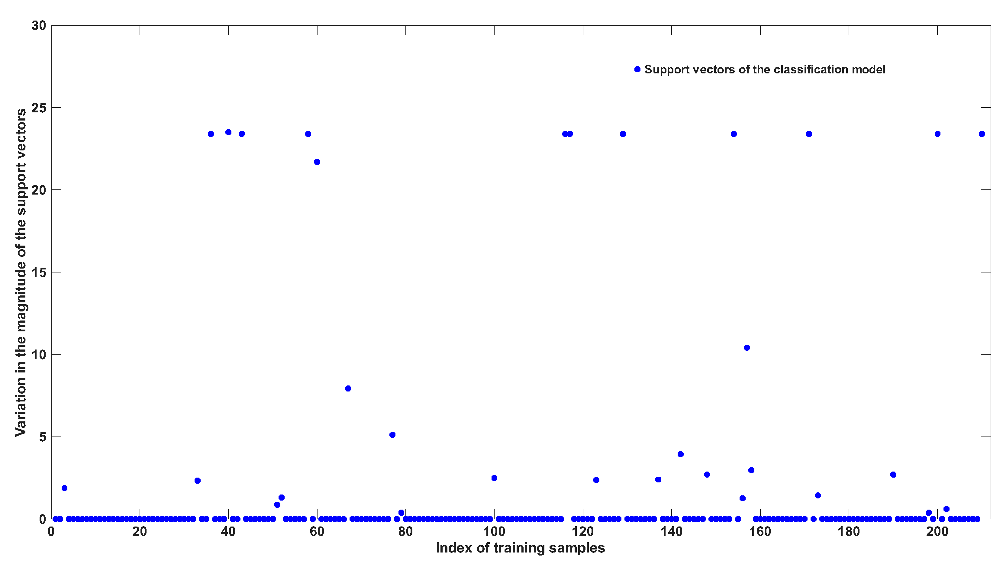
Table 3 summarizes the classification performance of SVM, LSSVM, and the proposed dual-norm method on the standard spiral dataset. Three metrics are reported: training accuracy, testing accuracy, and model sparsity. These metrics collectively assess the model’s predictive performance and structural compactness. These support vectors, accounting for 14.76% of the total, have non-zero coefficients ( α i + β i 0 ), and define the effective decision boundary, as shown in Figure 5. This highlights the effectiveness of the dual-norm regularization in promoting sparsity without sacrificing classification accuracy.
Next, to evaluate the effectiveness of the proposed method, experiments are conducted on a complex spiral dataset characterized by locally varying structures and intricate classification boundaries. The results are summarized in Table 4 and present the classification performance on the complex spiral dataset. The proposed dual-norm approach achieves a testing accuracy of 99.00%, which is slightly lower than that of LSSVM (100.00%) but higher than that of SVM (96.00%). Notably, it exhibits superior model sparsity at 32.14%, outperforming both SVM (23.33%) and LSSVM, which uses all training samples (0.00% sparsity). This demonstrates the dual-norm method’s ability to balance classification accuracy and model compactness more effectively.
The results highlight the advantage of the proposed dual-norm formulation. This benefit stems from the model structure: the α i coefficients control overall model sparsity, while the β i coefficients emphasize correction of extreme misclassifications. As a result, the dual-norm classifier constructs a sparse yet robust classification surface, which is particularly well-suited for data with intense local variations, such as the spiral patterns used in this study.

4.2. UCI Dataset

The binary classification task was evaluated on the well-known UCI Breast Cancer Wisconsin (Diagnostic) dataset [44]. This dataset consists of 569 instances, each described by 30 numerical features derived from digitized images of fine needle aspirate (FNA) of breast masses. Each instance is labeled as either malignant or benign, making it a standard benchmark for evaluating the classification performance of machine learning models in biomedical domains. In this experiment, 80% of the dataset was randomly selected for training, and the remaining 20% was used for testing.
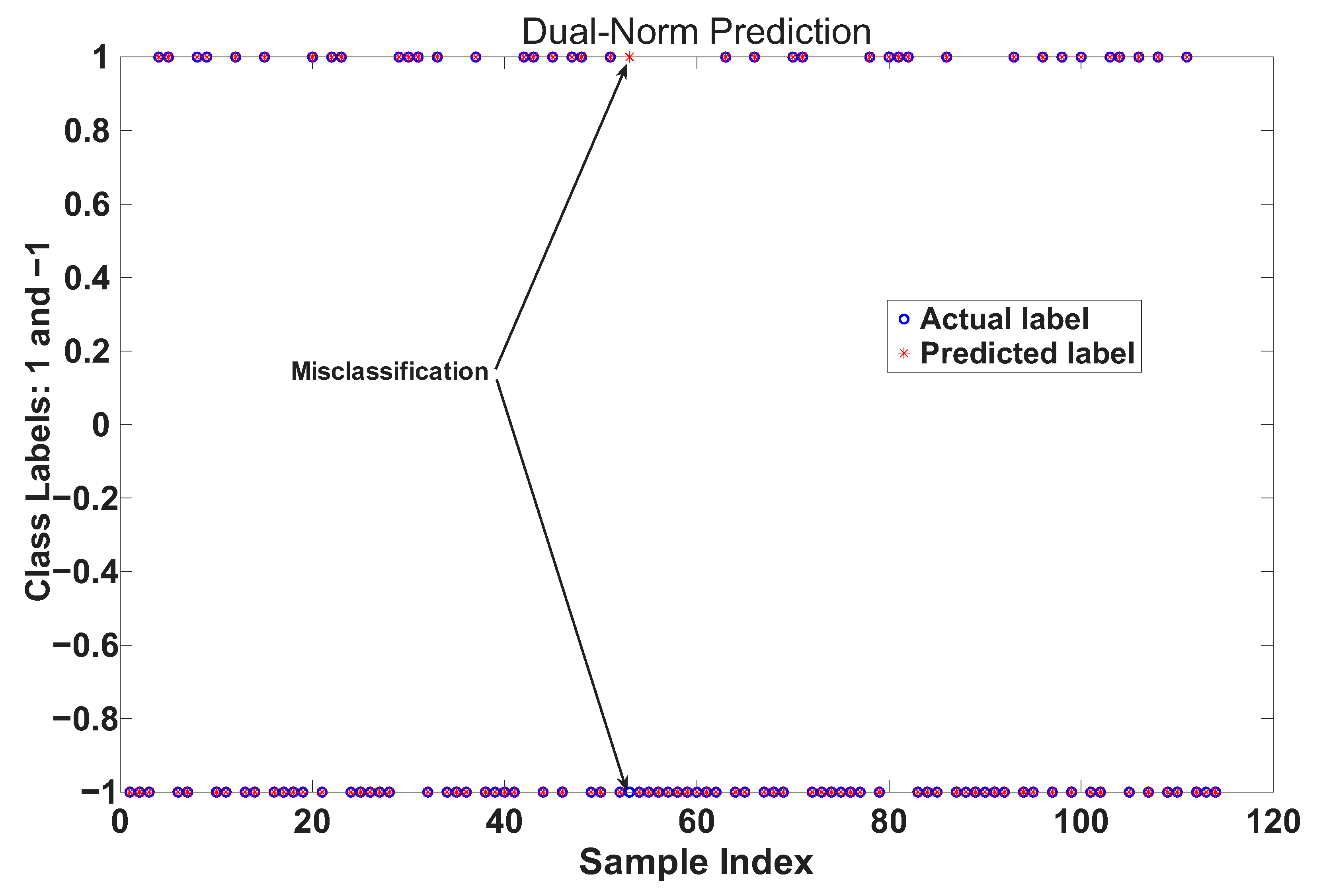
We compared the proposed dual-norm regularized classification model with standard support vector machine (SVM) and least squares SVM (LSSVM) on this dataset. The results include training accuracy, testing accuracy, and model sparsity. The comparative results are summarized in Table 5. The classification performance of the proposed dual-norm method, standard SVM, and LSSVM was evaluated on the test dataset. The dual-norm approach achieved a training accuracy of 98.68% and a testing accuracy of 95.61%, with a sparsity level of 92.97%, indicating that the majority of the dual variables were zero and the model is highly compact. In comparison, the standard SVM attained a similar training accuracy of 98.68%, a slightly lower testing accuracy of 94.74%, and a sparsity of 84.84%, reflecting a larger number of support vectors. The LSSVM achieved the highest training and testing accuracies of 99.12% and 96.49%, respectively, but exhibited no sparsity (0.00%), as all the training samples contributed to the model. These results demonstrate that the proposed dual-norm method provides a favorable balance between classification accuracy and model sparsity compared to SVM and LSSVM. These results highlight the superior performance of the dual-norm regularized model in balancing classification accuracy and model sparsity, making it particularly advantageous for interpretable and computationally efficient classification in biomedical applications. Further, we analyze the behavior of the dual-norm regularized model. Figure 6 is the test classification result, which visualizes the predicted class labels against the ground truth, showing a clear separation between benign and malignant samples. These visual results not only validate the model’s classification accuracy but also demonstrate its structural compactness, which is desirable for high-stakes biomedical decision-making systems that require transparency and robustness.
To comprehensively evaluate the proposed dual-norm SVM, we extended our experiments to include 12 widely-used benchmark datasets from the UCI repository, incorporating diverse data characteristics in terms of dimensionality, sample size, and class distribution. These range from low-dimensional examples such as Balance Scale (4 features) to higher-dimensional ones such as Ionosphere (34 features); from small datasets like Hepatitis (155 samples) to larger ones such as Banknote Authentication (1372 samples); several datasets, including Hepatitis and Haberman, also exhibit significant class imbalance. Each dataset was preprocessed uniformly, and hyperparameters were selected via five-fold cross-validation under consistent evaluation protocols. As summarized in Table 6, in which all experimental results are based on optimal parameters, the proposed method was compared against standard SVM and LSSVM based on training accuracy, test accuracy, and model sparsity (i.e., the proportion of non-zero support vectors). The results demonstrate that our approach achieves competitive or superior generalization performance across most datasets. For instance, it attains 94.29% test accuracy on the Transfusion dataset, outperforming SVM (91.43%) and LSSVM (96.19%); 90.00% on Raisin, exceeding LSSVM (87.78%) and matching closely with SVM (88.52%); and 84.78% on Hepatitis, significantly improving upon both baselines (80.44%). Moreover, the proposed method consistently yields sparser models—greatly reducing non-zero support vectors without sacrificing accuracy. On Cancer, it attains 97.14% test accuracy with only 10.63% non-zero support vectors, compared to LSSVM (88.98%) and SVM (19.22%). Similarly, on Transfusion, it uses only 32.93% non-zero support vectors versus SVM (72.36%) and LSSVM (100%). These results confirm that the proposed dual-norm SVM effectively balances predictive accuracy and model simplicity, demonstrating robustness across varying data dimensions, sizes, and imbalance ratios.
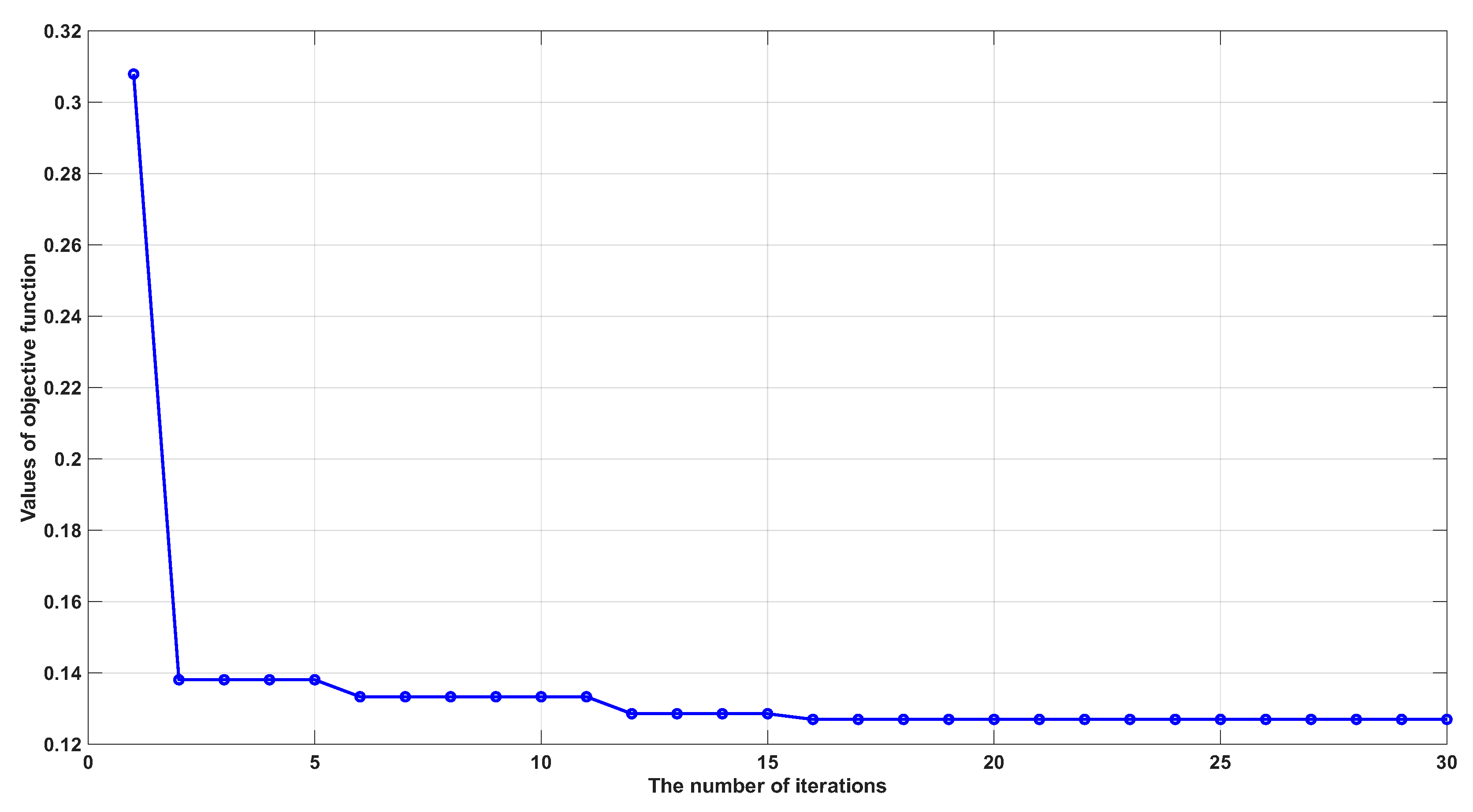
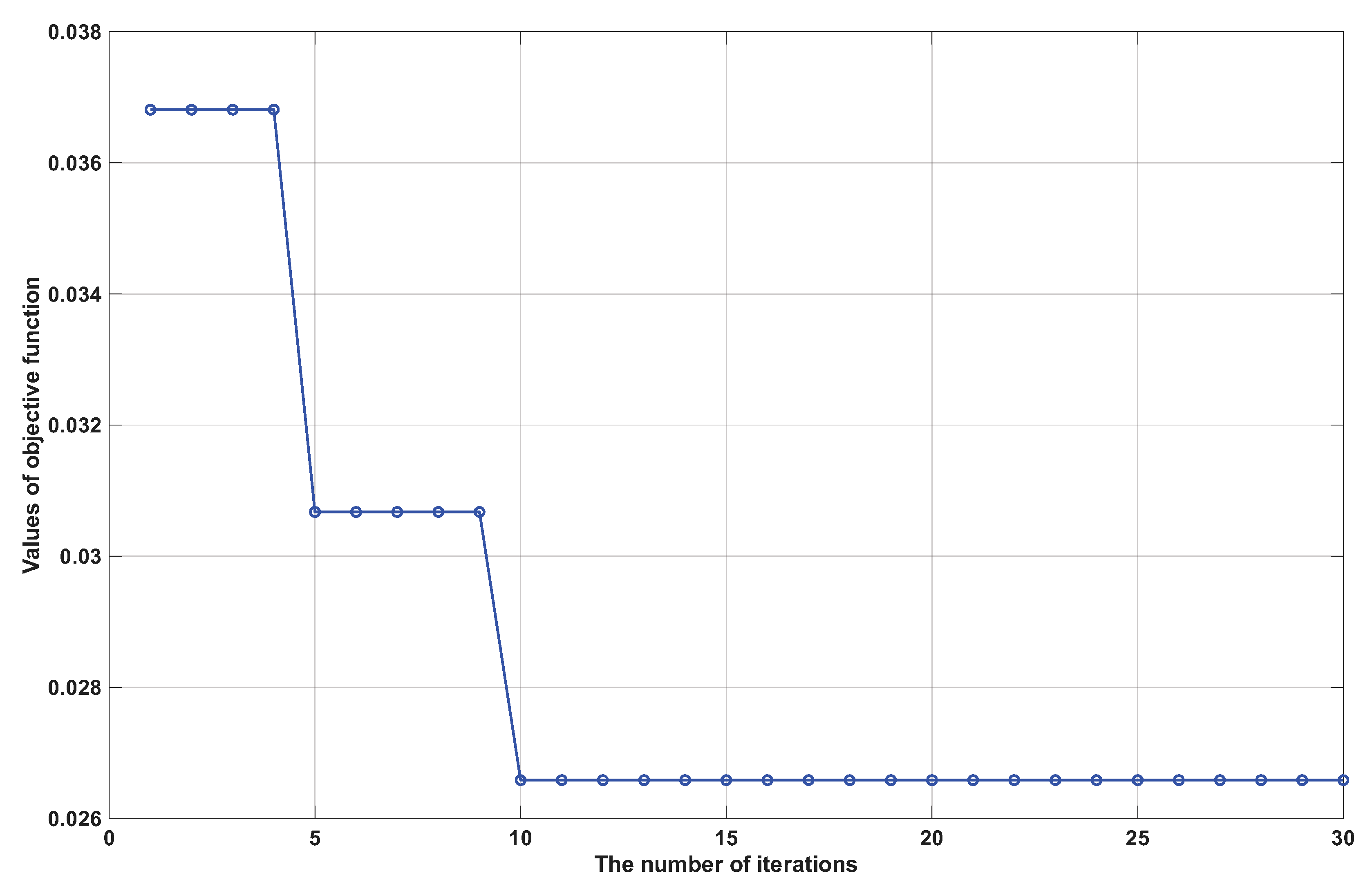
Next, the convergence behavior of the proposed method is further evaluated using two benchmark datasets: Raisin and Cancer. Figure 7 and Figure 8 illustrate the evolution of the objective function values across successive iterations of the optimization process. As shown, the algorithm consistently reaches the optimal solution within fewer than 15 iterations for both datasets. This observation confirms that the proposed iterative optimization scheme exhibits rapid and stable convergence, thereby demonstrating its computational efficiency and practical applicability in real-world scenarios.

5. Conclusions

This paper introduced a dual-norm support vector machine framework that integrates both L 1 and L slack penalties to achieve robust and sparse binary classification. By simultaneously minimizing the total misclassification error and the worst-case slack violation, the proposed method effectively balances average performance with robustness to outliers. The inclusion of the L -norm term enables explicit control over extreme margin violations, which are often overlooked in traditional SVM and LSSVM formulations.
The resulting convex optimization problem, governed by two hyperparameters C 1 and C 2 , maintains computational tractability while offering increased flexibility in tuning the trade-off between global accuracy and worst-case robustness. Experimental results on synthetic and real-world benchmark datasets demonstrate that the dual-norm classifier achieves competitive or superior classification accuracy compared to standard SVM and LSSVM approaches. Moreover, the proposed method consistently produces sparser models, enhancing interpretability and computational efficiency.
Overall, this study highlights the effectiveness of combining L 1 and L regularization in support vector classification, providing a principled approach to constructing classifiers that are not only accurate but also structurally compact and robust against extreme misclassifications. Future work may explore kernel extensions and multi-class generalizations of the dual-norm strategy.

Author Contributions

Conceptualization, X.L., X.Y., and C.Z.; methodology, G.Y. and X.L.; validation, X.L., S.L., and Q.L.; formal analysis, F.Z.; writing—original draft preparation, X.L. and Q.L.; writing—review and editing, X.L.; supervision, X.Y.; funding acquisition, X.Y. and X.L. All authors have read and agreed to the published version of the manuscript.

Funding

The research was funded by the Key Laboratory Project of the Guizhou Provincial Department of Education(QJJ[2023]029), the National Natural Science Foundation of China (61966006), the Zunyi Technology and Big Data Bureau, Moutai Institute Joint Science and Technology Research and Development Project (ZSKHHZ[2024] No.384, ZSKHHZ[2024] No.385, ZSKHHZ[2022] No.164) and training program of high-level innovative talents of Moutai institute (mygccrc[2024]011, mygccrc[2023]021, mygccrc[2022]100, mygccrc[2022]113, mygccrc[2024]012), Zunyi Science and Technology Innovation Team Project (KCTD065).

Data Availability Statement

The original contributions presented in this study are included in the article. Further inquiries can be directed to the corresponding author.

Conflicts of Interest

The authors declare no conflicts of interest.

References

  1. Suaarez, C.A.; Castro, M.; Leon, M.; Martin-Barreiro, C.; Liut, M. Improving SVM performance through data reduction and misclassification analysis with linear programming. Complex Intell. Syst. 2025, 11, 356. [Google Scholar] [CrossRef]
  2. Amaya-Tejera, N.; Gamarra, M.; Velez, J.I.; Zurek, E. A distance based kernel for classification via Support Vector Machines. Front. Artif. Intell. 2024, 7, 1287875. [Google Scholar] [CrossRef]
  3. Yang, C.Y.; Chen, Y.Z. Support vector machine classification of patients with depression based on resting state electroencephalography. Asian Biomed. 2024, 18, 212–223. [Google Scholar] [CrossRef]
  4. Boser, B.E.; Guyon, I.; Vapnik, V.N. A training algorithm for optimal margin classifiers. In Proceedings of the Fifth Annual Workshop on Computational Learning Theory, Pittsburgh, PA, USA, 27–29 July 1992; Volume 5, pp. 144–152. [Google Scholar]
  5. Cortes, C.; Vapnik, V. Support-vector networks. Mach. Learn. 1995, 20, 273–297. [Google Scholar] [CrossRef]
  6. Bennett, K.P.; Campbell, C. Support vector machines: Hype or hallelujah? ACM SIGKDD Explor. Newsl. 2000, 2, 1–13. [Google Scholar] [CrossRef]
  7. Tsang, I.W.; Kwok, J.T.; Cheung, P.M. Core vector machines: Fast SVM training on very large data sets. J. Mach. Learn. Res. 2005, 6, 363–392. [Google Scholar]
  8. Xu, H.; Caramanis, C.; Mannor, S. Robust support vector machine training via convex outlier ablation. J. Mach. Learn. Res.. 2009, 10, 1485–1510. [Google Scholar]
  9. Wang, S.; Chen, Z.; Hu, Y. Robust twin support vector machine for binary classification. Knowl.-Based Syst. 2014, 67, 186–195. [Google Scholar]
  10. Zhang, J.; Zhang, L.; Huang, Y. Nonconvex and robust SVM with bounded ramp loss. Inf. Sci. 2021, 546, 453–467. [Google Scholar]
  11. Yuan, X.; Zhang, J.; Li, Y. Sparse support vector machine modeling by linear programming. IEEE Trans. Neural Netw. Learn. Syst. 2019, 30, 1077–1090. [Google Scholar]
  12. Li, Y.; Zhao, X.; Wang, J. Robust SVM with bounded loss for handling noisy and imbalanced data. Pattern Recognit. 2022, 129, 108688. [Google Scholar]
  13. Suykens, J.A.K.; Vandewalle, J. Least squares support vector machine classifiers. Neural Process. Lett. 1999, 9, 293–300. [Google Scholar] [CrossRef]
  14. Suykens, J.A.K.; Gestel, T.V.; De Brabanter, J.; De Moor, B.; Vandewalle, J. Least Squares Support Vector Machines; World Scientific Publishing Company: Singapore, 2002. [Google Scholar]
  15. Khanjani Shiraz, R.; Babapour-Azar, A.; Hosseini Nodeh, Z.; Pardalos, P. Distributionally robust joint chance-constrained support vector machines. Optim. Lett. 2022, 17, 1–19. [Google Scholar] [CrossRef]
  16. Faccini, D.; Maggioni, F.; Potra, F.A. Robust and distributionally robust optimization models for linear support vector machine. Comput. Oper. Res. 2022, 147, 105930. [Google Scholar] [CrossRef]
  17. Lin, F.; Yang, J.; Zhang, Y.; Gao, Z. Distributionally robust chance-constrained kernel-based support vector machine. Comput. Oper. Res. 2024, 170, 106755. [Google Scholar] [CrossRef]
  18. Tagawa, K. A support vector machine-based approach to chance constrained problems using huge data sets. In Proceedings of the 52nd ISCIE International Symposium on Stochastic Systems Theory and its Applications, Osaka, Japan, 29–30 October 2020. [Google Scholar]
  19. Zhao, H.; Wang, Y.; Zhang, L. Robust LSSVM with adaptive Huber loss for noisy classification problems. Neural Process. Lett. 2022, 54, 2187–2202. [Google Scholar]
  20. Xu, J.; Wang, C. An improved LSSVM model with ϵ-insensitive pinball loss. Expert Syst. Appl. 2023, 213, 119203. [Google Scholar]
  21. Liu, X.; Zhang, S.; Jin, Y. A sparse LSSVM using 1-norm regularization for classification. Knowl.-Based Syst. 2021, 229, 107384. [Google Scholar]
  22. Sharma, R.; Suykens, J.A.K. Mixed-norm regularization in least squares support vector machines. IEEE Trans. Neural Netw. Learn. Syst. 2022, 33, 4711–4723. [Google Scholar]
  23. Chen, T.; Zhou, H.; Wang, J. A convex–concave hybrid algorithm for robust LSSVM training. Appl. Soft Comput. 2023, 132, 109865. [Google Scholar]
  24. Banerjee, A.; Ghosh, A. Sparse LSSVM via kernel pruning and proximal gradient optimization. Pattern Recognit. 2021, 112, 107759. [Google Scholar]
  25. Wang, R.; Li, Z.; He, X. Dual-norm regularized LSSVM for robust classification. Pattern Recognit. Lett. 2023, 167, 78–85. [Google Scholar]
  26. Huang, M.; Zhang, Y.; Liu, Q. Slack variable norm hybridization for improved generalization in SVM classifiers. Neurocomputing 2024, 547, 126271. [Google Scholar]
  27. Xu, L.; Neufeld, J.; Larson, B.; Schuurmans, D. Maximum margin clustering. Adv. Neural Inf. Process. Syst. 2004, 17, 1537–1544. [Google Scholar]
  28. Zhu, J.; Rosset, S.; Hastie, T.; Tibshirani, R. 1-norm support vector machines. Adv. Neural Inf. Process. Syst. 2004, 16, 49–56. [Google Scholar]
  29. Shen, X.; Wang, L. Adaptive model selection and penalization for high-dimensional linear models. Stat. Sin. 2014, 24, 1113–1135. [Google Scholar]
  30. Yang, M.S.; Su, C.H. A fuzzy soft support vector machine for classifying multi-class data. Expert Syst. Appl. 2010, 37, 682–685. [Google Scholar]
  31. Hong, Y.; Zhang, H.; Wu, X. Multi-kernel least squares support vector machine based on optimized kernel combination. Knowl.-Based Syst. 2020, 192, 105320. [Google Scholar]
  32. Zhang, W.; Guo, Y.; Liang, J.; Song, C. Robust least squares support vector machine based on adaptive loss function. Pattern Recognit. 2022, 125, 108556. [Google Scholar]
  33. Jiang, T.; Wei, B.; Yu, G.; Ma, J. Generalized adaptive Huber loss driven robust twin support vector machine learning framework for pattern classification. Neural Process. Lett. 2025, 57, 63. [Google Scholar] [CrossRef]
  34. Wang, H.; Zhang, Y.; Zhang, X.; Zhang, Y. Fast truncated Huber loss SVM for large scale classification. Knowl.-Based Syst. 2023, 191, 110074. [Google Scholar] [CrossRef]
  35. Liu, Q.; Zhu, W.; Dai, Z.; Ma, Z. Multi-task support vector machine classifier with generalized Huber loss. J. Classif. 2025, 42, 221–252. [Google Scholar] [CrossRef]
  36. Fang, K.; Zhang, J.; Zhang, Y. Structured sparse support vector machine with ordered penalty. J. Comput. Graph. Stat. 2020, 29, 1005–1018. [Google Scholar]
  37. Moosaei, H.; Tanveer, M.; Arshad, M. Sparse least-squares universum twin bounded support vector machine. Knowl.-Based Syst. 2024, 259, 107984. [Google Scholar]
  38. Wang, H.J.; Zhang, H.W.; Li, W.Q. Sparse and robust support vector machine with capped squared loss for large scale pattern classification. Pattern Recognit. 2024, 153, 110544. [Google Scholar] [CrossRef]
  39. Yuan, C.; Yang, L. Capped L2,p-norm metric based robust least squares twin support vector machine for pattern classification. Neural Netw. 2021, 142, 457–478. [Google Scholar] [CrossRef] [PubMed]
  40. Wang, H.; Yu, G.; Ma, J. WCTBSVM: Welsch loss with capped L2,p-norm twin support vector machine. Symmetry 2023, 15, 1076. [Google Scholar] [CrossRef]
  41. Zhu, W.; Song, Y.; Xiao, Y. Robust support vector machine classifier with truncated loss function by gradient algorithm. Comput. Ind. Eng. 2022, 171 Pt A, 108630. [Google Scholar] [CrossRef]
  42. Akhtar, M.; Tanveer, M.; Arshad, M. RoBoSS: A robust, bounded, sparse, and smooth loss function for supervised learning. IEEE Trans. Pattern Anal. Mach. Intell. 2024, 47, 149–160. [Google Scholar] [CrossRef]
  43. Bhardwaj, P.; Tiwari, P.; Olejar, K., Jr.; Parr, W.; Kulasiri, D. A machine learning approach for grape classification using near-infrared hyperspectral imaging. Expert Syst. Appl. 2021, 174, 114774. [Google Scholar]
  44. Dua, D.; Graff, C.; UCI Machine Learning Repository. University of California, Irvine, School of Information and Computer Sciences. 2019. Available online: https://archive.ics.uci.edu/ml/datasets/Breast+Cancer+Wisconsin+(Diagnostic) (accessed on 30 June 2025).
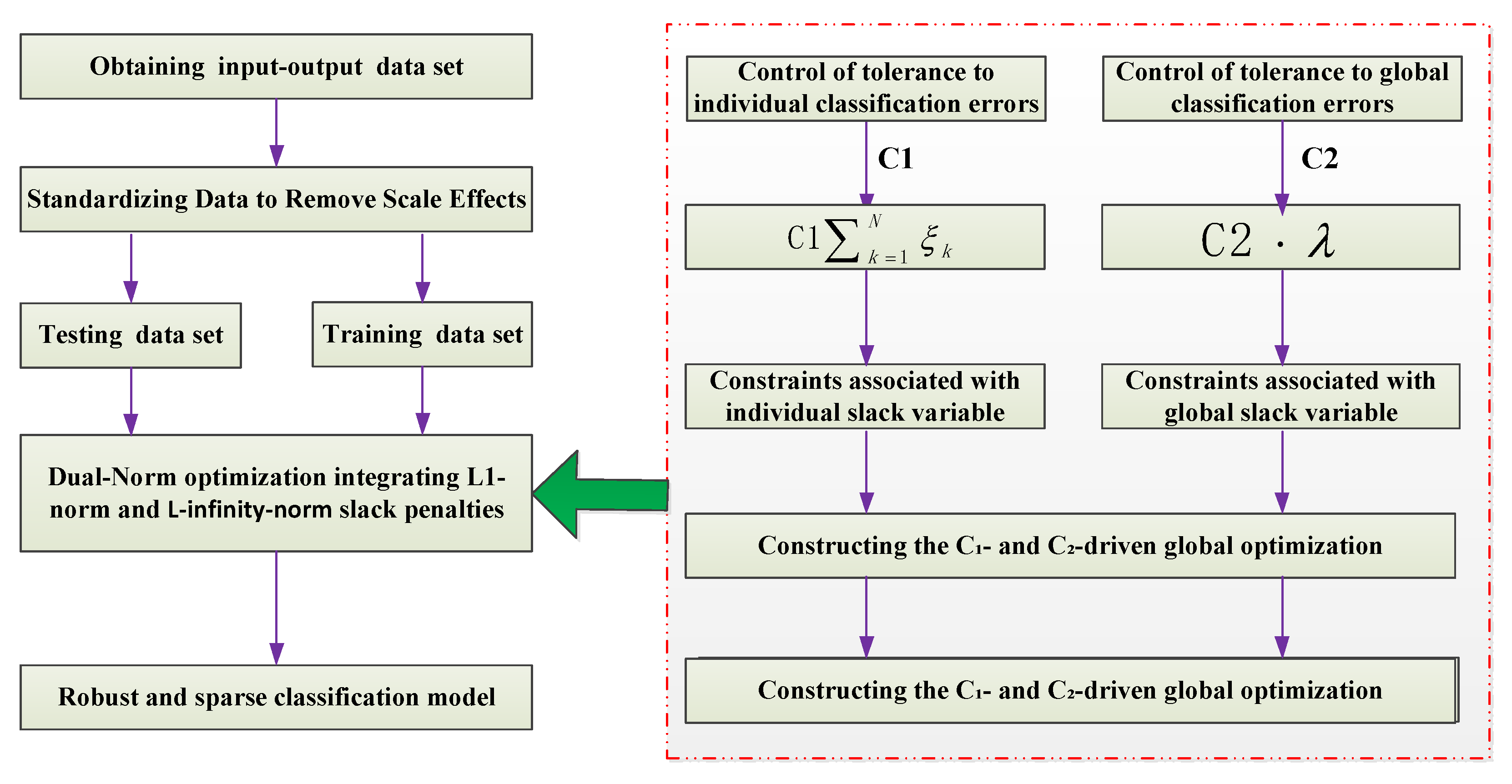
Figure 1. A concise flowchart for our approach.
Processes 13 02858 g001
Figure 2. The decision boundaries of the dual-norm regularized SVM for varying C 2 values while keeping C 1 fixed at 0.1.
Processes 13 02858 g002
Figure 3. The decision boundaries of the dual-norm regularized SVM for varying C 1 values with C 2 fixed at 10.
Processes 13 02858 g003
Figure 4. Predicted outputs of the dual-norm support vector classification method on the standard spiral dataset.
Processes 13 02858 g004
Figure 5. The distribution of the magnitudes of the model coefficients ( α + β ) corresponding to 31 support vectors is shown and all remaining magnitudes are zero.
Processes 13 02858 g005
Figure 6. Predicted outputs of the dual-norm support vector classification method on the standard spiral dataset.
Processes 13 02858 g006
Figure 7. The objective function values of the proposed method decrease as the iteration number increases on Raisin dataset.
Processes 13 02858 g007
Figure 8. The objective function values of the proposed method decrease as the iteration number increases on Cancer datasets.
Processes 13 02858 g008
Table 1. Roles of the regularization terms in the proposed optimization problem.
TermParameterFunctionEffect on ModelProblem Addressed
Local slack variables C 1 i = 1 N ξ i Allows individual samples to violate the marginControls classification accuracy vs. robustness: larger C 1 reduces misclassification but increases the number of support vectorsHandles local noise and outliers, stabilizes the decision boundary
Global slack variable C 2 λ Penalizes the global relaxation λ Controls sparsity: larger C 2 suppresses non-critical samples, reduces the number of support vectorsEnhances sparsity, reduces model complexity, ensures that the decision boundary is determined by key samples
Table 2. Comparison results for different C 1 and C 2 .
C 1 C 2 SV_Ratio β λ Training AccuracyTest Accuracy
0.0100.00%0.00.0096.0%95.00%
0.5100.00%0.51.04492.00%92.00%
1.0100.00%1.01.01091.00%93.00%
0.12.0100.00%2.01.00390.00%92.00%
5.0100.00%5.00.978100.00%92.00%
10.0100.00%10.00.79597.00%93.00%
0.076.00%0.00.097.00%95.00%
0.574.00%0.51.71896.00%95.00%
1.074.00%1.01.41196.00%95.00%
0.52.073.00%2.01.05094.00%98.00%
5.077.00%5.01.01595.00%97.00%
10.076.00%10.00.961100.00%96.00%
0.066.00%0.00.097.00%95.00%
0.567.00%0.52.00397.00%95.00%
1.066.00%1.01.88697.00%95.00%
1.02.067.00%2.01.34297.00%95.00%
5.067.00%5.01.02996.00%98.00%
10.065.00%10.00.983100.00%97.00%
0.060.00%0.00.098.00%95.00%
0.560.00%0.51.71298.00%95.00%
1.060.00%1.01.64498.00%95.00%
5.02.059.00%2.01.50698.00%95.00%
5.057.00%5.01.10498.00%96.00%
10.056.00%10.00.985100.00%96.00%
0.056.00%0.00.099.00%97.00%
0.557.00%0.51.49999.00%97.00%
1.057.00%1.01.43599.00%98.00%
10.02.057.00%2.01.30699.00%98.00%
5.056.00%5.01.01798.00%98.00%
10.055.00%10.00.990100.00%98.00%
Table 3. Comparison of classifier performance on the standard spiral dataset.
MethodTraining Accuracy (%)Testing Accuracy (%)Zero Sparsity (%)
SVM99.52100.0022.38
LSSVM99.52100.000.00
Dual-Norm99.52100.0084.76
Table 4. Comparison of classifier performance on the complex spiral dataset.
MethodTraining Accuracy (%)Testing Accuracy (%)Zero Sparsity(%)
SVM99.0597.7847.62
LSSVM99.0596.670.00
Dual-Norm99.0597.7885.24
Table 5. Classification performance comparison on the UCI Breast Cancer dataset.
MethodTraining AccuracyTest AccuracyZero Sparsity
LSSVM99.56%99.12%0.00%
SVM98.46%98.25%80.66%
Dual-Norm98.02%99.12%90.55%
Table 6. Classification performance comparison on the UCI dataset.
Datasets ( m × n )MethodTraining AccuracyTest AccuracyNon-Zero Sparsity
Balance ( 625 × 4 )LSSVM91.78% (402/438)91.44% (314/483)100.00% (438/438)
SVM100.00% (483/483)99.47% (186/187)20.40% (89/438)
Proposed100.00% (438/438)100.00% (187/187)20.40% (89/438)
Fisheriris ( 150 × 4 )LSSVM98.10% (104/105)93.33% (42/45)100% (100/100)
SVM99.05 % (104/105)95.56% (43/45)32.38% (34/105)
Proposed99.05% (104/105)95.56% (43/45)28.57% (30/105)
Australian ( 690 × 14 )LSSVM87.37% (422/483)90.34% (187/207)99.59% (481/483)
SVM86.34% (417/483)89.86% (186/207)65.01% (314/483)
Proposed86.54% (418/483)89.86% (186/207)64.18% (310/483)
ILPD ( 583 × 10 )LSSVM100.00% (409/409)71.84% (125/174)100.00% (409/409)
SVM100.00% (409/409)71.84% (125/174)65.01% (404/409)
Proposed90.22% (369/409)73.00% (127/174)64.18% (394/409)
Hepatitis ( 155 × 19 )LSSVM89.91% (98/109)80.44% (37/46)100.00% (109/109)
SVM89.91% (98/109)80.44% (37/46)41.28% (45/109)
Proposed96.33% (105/109)84.78% (39/46)56.88% (62/109)
Ionosphere ( 351 × 34 )LSSVM80.92% (424/524)76.79% (172/224)100.00% (524/524)
SVM81.30% (426/524)73.66% (165/224)70.42% (369/524)
Proposed94.72% (233/246)77.68% (174/224)60.69% (318/524)
Transfusion ( 748 × 4 )LSSVM100.00% (246/246)96.19% (101/105)100.00% (246/246)
SVM96.34% (237/246)91.43% (96/105)72.36% (178/246)
Proposed84.35% (442/524)94.29% (99/105)32.93% (81/246)
Wholesale ( 440 × 7 )LSSVM72.08% (222/308)71.21% (94/132)100.00% (308/308)
SVM100.00% (308/308)71.32% (94/132)66.88% (206/308)
Proposed72.08% (222/308)71.97% (95/132)73.05% (222/308)
Cancer ( 699 × 9 )LSSVM97.14% (475/489)96.19% (202/210)88.98% (440/489)
SVM97.14% (475/489)96.19% (202/210)19.22% (94/489)
Proposed97.34% (476/489)97.14% (204/210)10.63% (52/489)
Banknote ( 1372 × 4 )LSSVM100.00% (960/960)100.00% (412/412)100.00% (960/960)
SVM99.90% (959/960)99.51% (410/412)100.00% (960/960)
Proposed100.00% (960/960)100.00% (412/412)36.15% (347/960)
Haberman ( 306 × 3 )LSSVM76.64% (164/214)70.65% (65/92)100.00% (214/214)
SVM98.13% (210/214)66.30% (61/92)94.86% (203/214)
Proposed77.10% (165/214)69.57% (64/92)88.32% (189/214)
Raisin ( 900 × 7 )LSSVM87.14% (549/630)87.78% (237/270)100.00% (630/630)
SVM86.67% (546/630)88.52% (239/270)50.79% (320/630)
Proposed77.10% (165/214)90.00% (243/270)48.41% (305/630)
Disclaimer/Publisher’s Note: The statements, opinions and data contained in all publications are solely those of the individual author(s) and contributor(s) and not of MDPI and/or the editor(s). MDPI and/or the editor(s) disclaim responsibility for any injury to people or property resulting from any ideas, methods, instructions or products referred to in the content.