Abstract
Resonant acoustic technology utilizes low-frequency vertical harmonic vibrations to induce full-field mixing effects in processed materials, and it is regarded as a “disruptive technology in the field of energetic materials”. Although numerous scholars have investigated the mechanisms of resonant acoustic mixing, there remains a lack of parameter selection methods for improving product quality and production efficiency in engineering practice. To address this issue, this study employs phase-field modeling and fluid–structure coupling methods to numerically simulate the transport process of glycerol during resonant acoustic mixing. The research reveals the mass transfer mechanism within the flow field, establishes a liquid-phase distribution index for quantitatively characterizing mixing effectiveness, and clarifies the enhancement effect of fluid transport on solid particle mixing through particle tracking methods. Furthermore, parameter studies on vibration frequency and amplitude were conducted, yielding a critical curve for guiding parameter selection in engineering applications. The results demonstrate that Faraday instability first occurs at the fluid surface, generating Faraday waves that drive large-scale vortices for global mass transfer, followed by localized mixing through small-scale vortices. The transport process of glycerol during resonant acoustic mixing comprises three distinct stages: stable Faraday wave oscillation, rapid mass transfer during flow field destabilization, and localized mixing upon stabilization. Additionally, increasing either vibration frequency or amplitude effectively enhances both the rate and effectiveness of mass transfer. These findings offer theoretical guidance for optimizing process parameters in resonant acoustic mixing applications.
1. Introduction
Resonant acoustic mixing technology is a new type of bladeless full-field mixing technology that achieves uniform mixing of materials by applying low-frequency, high-intensity transient vibration excitation to the mixing container. Initially developed by the USSR in the 1960s, it rapidly advanced by 2000 and is characterized by safety and efficiency [1,2,3,4]. In 2008, the Resodyn Corporation developed a series of resonant acoustic mixing equipment of various models based on this technology. Since then, resonant acoustic mixing technology has been widely applied in multiple fields, including the preparation of propellant slurries for composite energetic materials (e.g., solid rocket propellants and high-energy PBX explosives) [5], the production of fuel cell anode supports [6], nanoparticle dispersion and uniform coating [7], the formulation of 3D inkjet printing slurries [8], catalytic chemical reactions [9], crystal granulation [10], and advancements in microfluidic technology [11].
In recent years, research on the mechanisms of resonant acoustic mixing has been gradually increasing. Andrews et al. [12] revealed the mechanisms behind mixing different materials. For solid–solid mixing, interparticle collisions are critical for uniformity of mixing. For solid–liquid mixing, acoustic streaming theory explains the process. For liquid–liquid or gas–liquid mixing, Faraday waves drive flow instability and mixing. However, these mechanistic studies were only discussed from a macroscopic perspective, without systematic investigation. Zhang [13,14] employed the discrete element method to study the mechanism of solid particle mixing, finding that the process primarily relies on convection, and further investigated the effects of particle cohesion, vibration parameters, and wall–particle friction on mixing uniformity. Liu [15] analyzed the deagglomeration mechanism of ultrafine powders under different vibration parameters based on a force-balance model. When mixing viscous fluids using resonant acoustic devices, Wright et al. [16] proposed that mixing is mainly achieved through intense boundary interactions induced by surface disturbances and bulk acoustic streaming. Zhan et al. [17,18] studied the flow patterns and power consumption of high-viscosity fluids in resonant acoustic mixing, clarifying the influence of “mixing forces” composed of pressure and viscous forces under acoustic vibration on mixing efficiency. Claydon et al. [19,20] investigated the resonant acoustic mixing process of PBX simulants, finding that mixing efficiency primarily depends on materials’ displacement amplitude and the degree to which the “no-slip wall boundary condition” is satisfied. Huo [21,22,23] employed a phase-field model to study the mixing of power-law non-Newtonian fluids. The process was split into two stages. The first stage involved initial global fluid motion driven by Faraday waves. The second stage involved energy transfer and local mixing through vortex evolution. These studies systematically elucidated the mechanisms of resonant acoustic mixing for both solid particles and fluids, supplementing and refining the mechanisms proposed by Andrews et al. However, in practical engineering, the selection of vibration parameters is crucial for determining product quality and production efficiency, making it particularly important to develop a rapid and effective parameter selection method based on mixing mechanisms.
Meanwhile, against the backdrop of high experimental costs and technical limitations, numerical simulation methods for studying the mixing characteristics of gas–liquid two-phase flow systems have emerged. The primary challenges lie in interfacial discontinuity and multiscale phenomena. These methods can be broadly categorized into the Volume of Fluid (VOF) method, Level Set method, and phase field method [24,25,26]. Although sharp-interface methods like VOF and Level Set have received widespread attention, the VOF method involves a complex and computationally expensive interface reconstruction, while the Level Set method suffers from non-conservation and mass loss issues. In contrast, the phase field method captures phase interfaces based on free energy theory, accounting for topological changes and interfacial stress effects [27,28,29,30], making it a cost-effective and conservative diffuse-interface approach. On the other hand, selecting an appropriate turbulence model is equally crucial in numerical simulations. Common flow field simulation methods fall into three main categories: Direct Numerical Simulation (DNS), Large Eddy Simulation (LES), and Reynolds-Averaged Navier–Stokes (RANS) [31]. DNS solves the Navier–Stokes equations directly to simulate the evolution of all instantaneous turbulent motions, offering the highest accuracy but requiring extremely fine grids and substantial computational resources [32]. LES employs a filtering function to separate large-scale and small-scale eddies, directly resolving large eddies while modeling small-scale ones [33], thereby accurately capturing vortex evolution. However, as a relatively new numerical approach, LES is not well-suited for multiphase flows and is primarily limited to single-phase applications. RANS, on the other hand, applies turbulence statistical theory to average the Navier–Stokes equations and closes the Reynolds-averaged equations using empirical or semi-empirical constitutive relations derived from theory or experiments [34]. This method imposes lower computational requirements and has been widely applied in multiphase flow studies.
In summary, to provide more targeted guidance for practical production, this study first employs a phase-field model coupled with fluid–structure interaction to numerically simulate the transport process of glycerol in resonant acoustic mixing. The simulation is validated through grid independence analysis and flow pattern comparison experiments to elucidate the mass transfer mechanism in the flow field. Subsequently, based on the constructed liquid-phase distribution index, the mass transfer efficiency of the flow field is quantitatively characterized, and its enhancement effect on solid particle mixing is clarified using particle tracking methods. Finally, parameter studies focusing on vibrations’ frequency and amplitude under typical operating conditions are conducted to investigate their influence on flow field mass transfer, leading to the fitting of critical curves that can guide parameter selection in engineering applications.
2. Methods and Theory
Resonant acoustic mixing equipment achieves safe and efficient mixing of materials through vertical sinusoidal excitation applied to the container bottom. Since the resonant acoustic mixing container is a centrally symmetric cylinder and to save computational resources, this study simplifies the three-dimensional model by constructing a two-dimensional physical field model based on the axial cross-section of the cylinder, as shown in Figure 1.
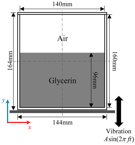
Figure 1.
Two-dimensional physical field model.
In Figure 1, the gray region represents glycerol, while the white region denotes air, with Corning glass constituting the wall material. The container has a diameter of 144 mm, height of 164 mm, and wall thickness of 2 mm, with a glycerol liquid level height of 96 mm. Furthermore, this study selects a parameter combination of vibration amplitude (8 mm) and frequency (60 Hz) as the representative operating condition [17,20,23]. Vibration velocity and vibration acceleration can be obtained by taking the first and second derivatives of the container displacement, respectively, as shown below:
where is the amplitude of vibration velocity, and is the amplitude of vibration acceleration.
The operation of a resonant acoustic mixing system can be simplified as an underdamped driven harmonic oscillator, where the relationship between acceleration and driving force is expressed as [20]
where is the mass of the system, is the displacement of the container, is the damping coefficient, is the spring constant, is the peak driving force, and is the driving force (resonant) frequency. Since the resonant frequency is determined solely by the inherent properties of the system (mass and stiffness) and is independent of external excitation and damping, it is theoretically feasible to mix high-viscosity fluids using resonant acoustic mixing technology.
This study uses a phase-field model. It simulates the two-phase flow characteristics of air and glycerol. The Cahn–Hilliard equation describes the dynamic behavior of this two-phase flow. It tracks the diffuse interface between two immiscible fluids. It also characterizes their evolution process. The diffuse interface is defined by a dimensionless phase-field variable . This variable varies continuously from −1 to 1. The Cahn–Hilliard equation is expressed as
where
where is the phase field variable, is the velocity vector, is the mobility, is the mixing energy density, is the interface thickness parameter, is the phase-field auxiliary variable, is the mobility adjustment parameter, and is the surface tension coefficient. Here, the parameters and are related through the surface tension coefficient , as shown below:
The volume fraction of the fluid inside the container is given by
where the subscripts and N represent air and non-Newtonian fluid, respectively. The density and viscosity of the mixture at the phase interface are given by
The continuity equation and the incompressible Navier–Stokes equations are shown below:
where
where is the pressure, is the equivalent gravitational acceleration, is the surface tension, is the gravitational acceleration, and is the unit vector along the y-axis.
This study employs the standard model, which is suitable for simulating high Reynolds number, shear-dominated turbulence induced by high-frequency vibrations in the resonant acoustic mixing process. This model can effectively capture the evolution of vortex structures and energy dissipation in the main regions of the flow field, and it also exhibits high computational efficiency. The turbulent viscosity is calculated by solving transport equations. These equations describe turbulent kinetic energy and dissipation rate . This step closes the RANS equations. The transport equations are given by
where
where is the turbulent eddy viscosity coefficient, is the stress source term due to velocity gradients, and , , , , are empirical constants.
The dynamic governing equation for the container wall under oscillatory loading is expressed as
where the subscript denotes the container wall, is the displacement vector, is the stress tensor, and is the body force.
The fluid–structure interaction process involves two key aspects. One is the load glycerol exerts on the container walls. The other is the velocity the walls transmit to the fluid. These aspects are described by the following governing equations:
where I is the identity matrix, and n is the normal vector.
3. Numerical Simulation
For the established two-dimensional physical field model, meshing was performed on both the fluid domain and wall domain, as illustrated in Figure 2. The container walls were discretized using triangular unstructured grids, while quadrilateral structured grids were employed for the fluid domain, where higher computational accuracy was required, with an initial mesh size of 1 mm. To account for boundary layer effects in near-wall regions due to turbulence, the grid size was proportionally varied with wall distance, using a scaling factor of 10. The computed y+ (dimensionless distance from the first grid layer’s center to the wall) value of 37 satisfies the requirements for standard turbulence modeling (the ideal range of y+ values is 30–300) [35].
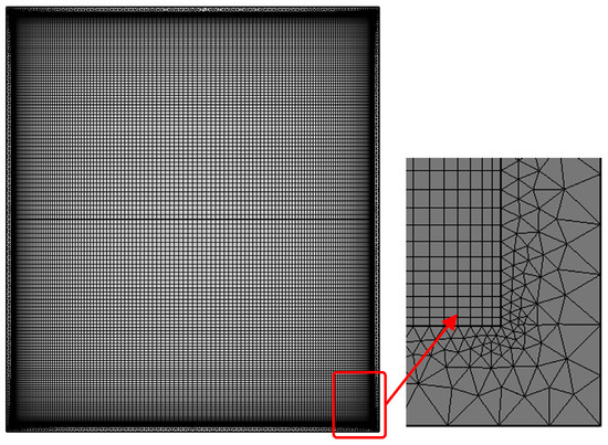
Figure 2.
Mesh generation.
The mesh density significantly influences the accuracy of numerical simulation results, necessitating mesh independence verification. The grid numbers in both x- and y-directions of the fluid domain were refined with a refinement factor of 1.5, resulting in five distinct mesh configurations. The time-averaged velocity during the first 1 s of flow field computation is shown in Figure 3. Analysis reveals that simulation errors demonstrate marked convergence tendencies with increasing mesh density. When the grid count reaches 35,497, the relative error decreases to 0.7%, meeting engineering accuracy requirements. Consequently, this study adopts this optimal mesh configuration for subsequent simulations, achieving optimal computational resource allocation while ensuring numerical precision.
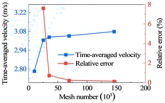
Figure 3.
Grid independence verification.
The mesh density critically determines numerical simulations’ accuracy, making grid independence analysis essential. The fluid domain was systematically refined by a factor of 1.5 in both x- and y-directions, generating five distinct mesh resolutions. Time-averaged velocity profiles during the initial 1 s flow development were computed and are presented in Figure 3. The analysis demonstrates a pronounced error reduction with refinement of the mesh, exhibiting clear convergence characteristics. At the optimal mesh count of 35,497 elements, the relative error diminishes to 0.7%, fulfilling engineering accuracy criteria. This validated mesh configuration was consequently adopted for subsequent simulations, achieving optimal computational efficiency without compromising the reliability of the results.
Building upon the established two-dimensional physical field model and determined mesh configuration, numerical simulations were performed using COMSOL Multiphysics 6.3 finite element software, with detailed parameter settings summarized in Table 1.

Table 1.
Numerical simulation settings.
To systematically investigate the influence of vibrations’ frequency and amplitude on flow field mass transfer, simulations were conducted across frequency ranges of 10–100 Hz (in 10 Hz increments) and amplitude ranges of 1–10 mm (in 1 mm increments), resulting in a total of 100 vibration parameter combinations, with the vibration velocity (m·s−1) and acceleration (m·s−2) corresponding to each combination listed in Table 2 and Table 3.
Table 2.
Vibration velocity (m·s−1) under different parameter combinations.
Table 3.
Vibration acceleration (m·s−2) under different parameter combinations.
4. Results and Discussion
4.1. Mass Transfer Mechanism
To visualize the flow dynamics of glycerol within the resonant acoustic container, volume fraction contours at different time points are extracted as shown in Figure 4, where blue represents glycerol, and red denotes air. The analysis reveals that at t = 0.06 s, multiple ligament structures (also referred to as Faraday waves) form at the glycerol–air interface. Previous studies [36] have demonstrated these Faraday waves constitute the primary instability mechanism in such flow fields. By t = 0.068 s, the ligament structures propagate toward the container top under inertial forces, subsequently undergoing tip breakup due to surface tension. At t = 0.075 s, new ligament structures emerge from the glycerol surface, continuing to transport fluid from the container bottom upward. When t = 1 s is reached, the entire fluid volume participates in global circulatory transport, significantly enhancing mass transfer efficiency within the flow field.
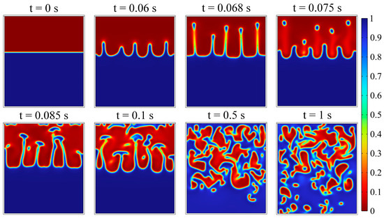
Figure 4.
Volume fractions of glycerol and air.
To further validate the numerical simulation’s accuracy, comparative experiments were conducted focusing on the flow pattern characteristics during glycerol mixing. The experimental setup is shown in Figure 5. We used a FASTCAM Mini UX50 high-speed camera. Its resolution was 1280 × 1024 pixels. The frame rate was 1000 fps. This camera captured how the flow patterns changed over time during the mixing process.
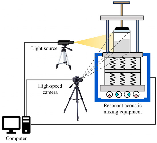
Figure 5.
Schematic diagram of the experimental setup.
Figure 6 shows the dynamic evolution law of flow patterns of glycerin during vibration, corresponding to the four time points in Figure 4. It can be observed that the trends of flow pattern evolution from numerical simulations and experimental results are generally consistent. The numerical simulation shows fewer Faraday waves and ligament structures than observed in experiments. Two main reasons explain this. First, the simulation uses a 2D model. It only captures features of one specific plane in 3D space. A 3D model would likely increase these structures. Second, the experiments involve random perturbations. These perturbations cause flow field fluctuations. This worsens fluid instability. It promotes more Faraday waves and ligament structures. Despite these differences, the main flow field structures match between simulation and experiment. The impact of these discrepancies on the study’s conclusions is acceptable. This fully validates the numerical simulation method used.
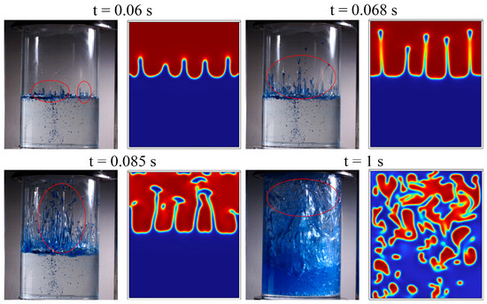
Figure 6.
Experimental validation (the red circle indicates the flow pattern features that are relatively similar to the numerical simulation results).
It should be noted that although the study focuses solely on gas–liquid two-phase flow, elucidating its mass transfer mechanism provides valuable insights for understanding gas–liquid–solid three-phase flows containing ultrafine powders. This is because ultrafine powders with micrometer-scale particle sizes predominantly follow the fluid flow behavior in the flow field [37]. Figure 7 presents the motion trajectories of aluminum particles in the resonant acoustic mixing flow field obtained using the particle tracing method. At the initial moment, the aluminum particles are released at the bottom of the container at a height of 10 mm. Observations reveal that under the action of Faraday waves, the aluminum particles gradually diffuse toward the top of the container, indicating that global fluid circulation can effectively promote the mixing of solid particles.
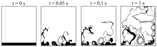
Figure 7.
Trajectories of aluminum particles.
To further investigate the mass transfer mechanism, velocity vector fields corresponding to the same time points in Figure 6 were extracted, as shown in Figure 8. The analysis reveals that flow instability initially occurs at the gas–liquid interface (t = 0.06 s), with the unstable region progressively expanding toward the container bottom over time, thereby engaging more fluid in global transport. Furthermore, the vortex structures identified from velocity vectors demonstrate that mass transfer is primarily achieved through large-scale vortices (t = 0.075 s) for whole-field transport and small-scale vortices (t = 1 s) for local mixing. In summary, the resonant acoustic mass transfer mechanism follows three distinct stages: Faraday instability first develops at the fluid surface; the flow field then establishes large-scale vortices under Faraday wave action to facilitate global mass transfer; and finally localized mixing is achieved through small-scale vortices.
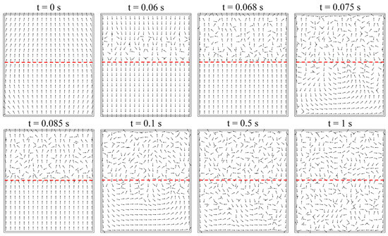
Figure 8.
Velocity vector of the flow field (the red dashed line represents the initial gas–liquid interface).
Since the container operates under resonant conditions during mass transfer, significant mechanical stresses develop at the walls, necessitating quantitative analysis. Figure 9 presents the wall stress distribution at different time instants, revealing stress concentrations primarily at the sidewalls and top surface, with maximum values occurring at the two top corners. This phenomenon results from continuous impingement of ligament structures on the container top during mass transfer. Furthermore, the observed trend of initial stress increase followed by reduction correlates directly with the mass transfer process: rapid whole-container mass transfer induces peak stresses during initial global fluid motion, followed by stress’s alleviation during subsequent localized mixing phases.
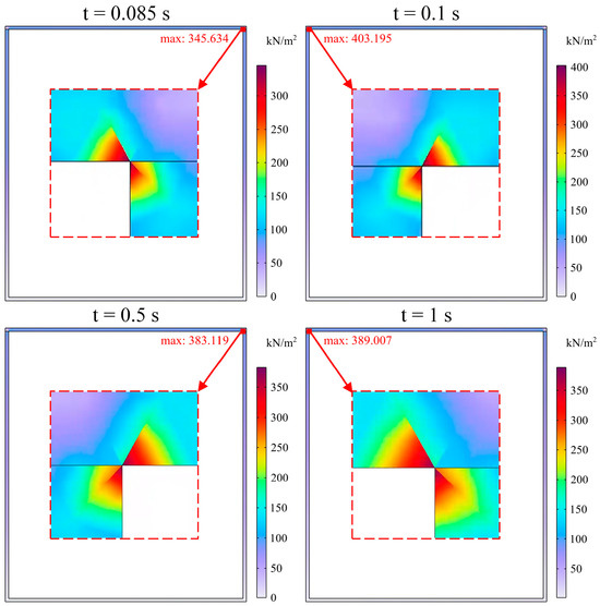
Figure 9.
Wall stress distribution of the container.
4.2. Effects of Vibration Frequency and Amplitude on Flow Field Mass Transfer
This study quantitatively characterizes mass transfer efficiency and rates in the flow field using a liquid-phase distribution index [38]. Since both the flow field space and fluid volume fraction are two-dimensional continuous functions, the liquid-phase distribution index is defined through an inner product formulated using functional norms:
where is the domain of the container, is the volume fraction of the glycerol at any given time, is the initial volume fraction, and is the volume fraction when the fluid is completely mixed uniformly, which is set to 0.5. The slope of the index represents the rate at which glycerol tends to distribute uniformly, while the magnitude indicates the degree of uniformity in glycerol’s distribution. Based on the previous analysis, the distribution of glycerol has a promoting effect on the transportation and transfer of particles; therefore, the glycerol distribution index can indirectly reflect the mass transfer efficiency of the flow field.
Figure 10 shows the liquid-phase distribution index under typical operating conditions, revealing three characteristic stages: (I) initial slow variation, (II) subsequent rapid ascent, and (III) final stabilization. Cross-referencing with Figure 6, Stage I corresponds to Faraday waves’ formation at the fluid surface, while the flow field remains stable without nonlinear instability, preventing wave propagation upward. Stage II begins with development of flow instability, where fluid continuously impacts the container top under Faraday wave action, driving global mass transfer. Stage III features localized mixing dominated by small-scale vortices, causing the distribution index to asymptotically approach equilibrium.
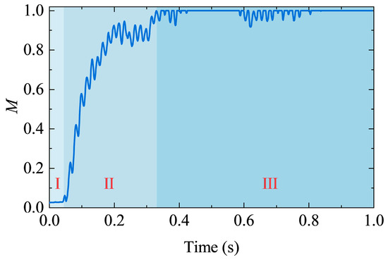
Figure 10.
Liquid-phase distribution index under typical operating conditions.
To further investigate the influence of vibrations’ frequency and amplitude on flow field mass transfer, the liquid-phase distribution indices under various parameter combinations were calculated as shown in Figure 11 and Figure 12. Figure 11 demonstrates that both mass transfer rate and efficiency improve with increasing vibration frequency, attributable to greater participation of fluid in global transport per unit time at higher frequencies. This phenomenon confirms that enhancing vibrations’ frequency effectively optimizes flow field transport characteristics. Notably, when the frequency reaches 60 Hz, the trend of index variation becomes statistically insignificant. While a further frequency increase would accelerate mass transfer, the 60 Hz condition represents the optimal operational point that maximizes energy efficiency while maintaining the required mass transfer performance, making it recommended for industrial applications.
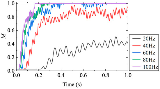
Figure 11.
Effect of vibration frequency on the liquid-phase distribution index.
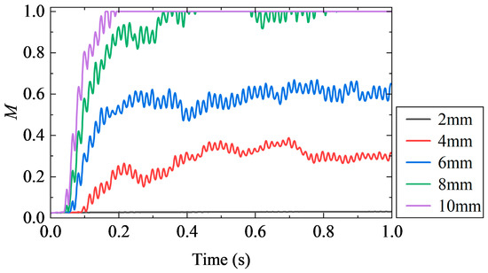
Figure 12.
Effect of vibration amplitude on the liquid-phase distribution index.
As shown in Figure 12, both the mass transfer rate and efficiency progressively improve with increasing amplitude of vibration, as larger amplitudes enhance the Faraday wave’s capacity to transport more fluid toward the container top per cycle. Compared with vibrations’ frequency, amplitude exerts greater influence on mass transfer: at 2 mm amplitude, the liquid-phase distribution index remains nearly constant, whereas optimal mass transfer occurs at 8 mm amplitude. Consequently, small-amplitude/high-frequency combinations should be avoided in parameter selection. An 8 mm amplitude represents the practical optimum—while a further amplitude increase would marginally reduce transfer duration, the diminishing returns cannot justify the substantially higher energy consumption, making the 8 mm condition the most operationally viable.
Although Figure 11 and Figure 12 demonstrate the liquid-phase distribution index under various vibration frequencies and amplitudes, the rapid and effective selection of optimal parameter combinations remains challenging. To address this, a confusion matrix was constructed based on statistical analysis of 100 simulation datasets, using the maximum liquid-phase distribution index as the evaluation metric, as shown in Figure 13. The results reveal a progressive enhancement in mass transfer efficiency from the lower-left to upper-right regions of the matrix.
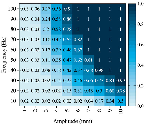
Figure 13.
Parameter efficiency matrix of the liquid-phase distribution index.
In practical applications, Figure 13 enables rapid parameter selection, yet accurate mass transfer evaluation remains challenging for extended parameter ranges or intermediate conditions between adjacent data points in the matrix. To resolve this limitation, we established a 0.9 liquid-phase distribution index as the threshold for ideal mass transfer. By selecting parameter sets near this threshold from Figure 13 and performing nonlinear fitting, we derived a critical demarcation curve separating optimal and suboptimal mass transfer regions. The curve’s mathematical expression is given by
The critical curve follows a power-law function, showing agreement with the findings of Zhan et al. [39]. As demonstrated in Figure 14, parameter combinations plotted above the curve indicate efficient mass transfer in the flow field, while those below the curve correspond to suboptimal mass transfer performance.

Figure 14.
Critical curve.
5. Conclusions and Perspectives
This study employs a phase-field model coupled with fluid–structure interaction to numerically simulate the transport processes of glycerol in resonant acoustic mixing, elucidating the underlying mass transfer mechanisms. Through development of a liquid-phase distribution index for quantitative characterization of transfer efficiency and particle tracking analysis demonstrating fluid-driven enhancement of solid particle mixing, we systematically investigated vibration parameters (frequency/amplitude) to derive engineering-critical performance curves. Three principal conclusions emerge:
- (1)
- The mass transfer mechanism of glycerol in resonant acoustic mixing proceeds through three distinct phases: (i) initial development of Faraday instability at the fluid surface, (ii) subsequent generation of large-scale vortices driven by Faraday waves enabling whole-field mass transport, and (iii) final achievement of localized mixing through small-scale vortices.
- (2)
- The transport process of glycerol in resonant acoustic mixing evolves through three characteristic stages: (i) stable Faraday wave oscillation, (ii) rapid mass transfer during flow instability, and (iii) localized mixing upon reaching steady state.
- (3)
- Both increasing vibrations’ frequency and amplitude effectively enhance the mass transfer rate and efficiency. The critical curve derived from parametric studies follows a power-law function.
Future research should incorporate multi-parametric critical curve calculations encompassing diverse fluid types, which would significantly enhance engineering guidance. Additionally, due to limited computational resources, this study conducted a numerical simulation of a 2D flow field in resonant acoustic mixing of glycerol. If conditions permit, the accuracy of the numerical simulation could be further improved by establishing a 3D model.
Author Contributions
Conceptualization, N.M.; methodology, N.M.; software, N.M.; validation, Y.G. and S.Z.; formal analysis, X.Z.; investigation, N.M.; resources, N.M.; data curation, X.Z.; writing—original draft preparation, N.M.; writing—review and editing, G.Z.; visualization, N.M.; supervision, G.Z.; project administration, X.Z.; funding acquisition, N.M. All authors have read and agreed to the published version of the manuscript.
Funding
This work was supported by the National Natural Science Foundation of China (Grant No. 52075413 and Grant No. 52475126).
Data Availability Statement
Data that support the findings of this study are available from the corresponding author upon reasonable request.
Conflicts of Interest
The authors declare that they have no known competing financial interests or personal relationships that could have appeared to influence the work reported in this paper.
References
- Abiev, R.S.; Vdovets, M.; Romashchenkova, N.; Maslikov, A. Intensification of mass transfer processes with the chemical reaction in multi-phase systems using the resonance pulsating mixing. Russ. J. Appl. Chem. 2019, 92, 1399–1409. [Google Scholar] [CrossRef]
- Karpacheva, S.; Zakharov, E.; Raginsky, L.; Muratov, V. Pul’siruyushchiye Ekstraktory; Atomizdat Moscow: Moscow, Russia, 1964. [Google Scholar]
- Karpacheva, S.; Zakharov, E. Osnovy Teorii i Rascheta Pul’satsionnykh Kolonnykh Reaktorov (Fundamentals of the Theory and Design of Pulsed Columnar Reactors); Atomizdat: Moscow, Russia, 1980. [Google Scholar]
- Karpacheva, S.; Ryabchikov, B. Pul’satsionnaya Apparatura v Khimicheskoi Tekhnologii; Khimiya Moscow: Moscow, Russia, 1983. [Google Scholar]
- Coguill, S.; Martineau, Z.; Martineau, Z. Vessel Geometry and Fluid Properties Influencing Mix Behavior for ResonantAcoustic Mixing Processes. In Proceedings of the 38th International Pyrotechnics Seminar, Denver, CO, USA, 10–15 June 2012; pp. 10–15. [Google Scholar]
- Park, J.H.; Bae, K.T.; Kim, K.J.; Joh, D.W.; Kim, D.; Myung, J.-H.; Lee, K.T. Ultra-fast fabrication of tape-cast anode supports for solid oxide fuel cells via resonant acoustic mixing technology. Ceram. Int. 2019, 45, 12154–12161. [Google Scholar] [CrossRef]
- Kevadiya, B.D.; Zhang, L.; Davé, R.N. Sustained Release of Poorly Water-Soluble Drug from Hydrophilic Polymeric Film Sandwiched Between Hydrophobic Layers. AAPS Pharmscitech 2018, 19, 2572–2584. [Google Scholar] [CrossRef] [PubMed]
- Effaty, F.; Gonnet, L.; Koenig, S.G.; Nagapudi, K.; Ottenwaelder, X.; Friscic, T. Resonant acoustic mixing (RAM) for efficient mechanoredox catalysis without grinding or impact media. Chem. Commun. 2023, 59, 1010–1013. [Google Scholar] [CrossRef]
- Gonnet, L.; Lennox, C.B.; Do, J.L.; Malvestiti, I.; Koenig, S.G.; Nagapudi, K.; Friscic, T. Metal-Catalyzed Organic Reactions by Resonant Acoustic Mixing. Angew. Chem. Int. Ed. Engl. 2022, 61, e202115030. [Google Scholar] [CrossRef]
- Liao, D.; Liu, Q.; Li, C.; Liu, N.; Wang, M.; An, C. RDX crystals with high sphericity prepared by resonance acoustic mixing assisted solvent etching technology. Def. Technol. 2023, 28, 23–32. [Google Scholar] [CrossRef]
- Zhang, S.; Zhan, L.; Zhang, Y.; Hou, J.; Li, B. Continuous flow resonance acoustic mixing technology: A novel and efficient strategy for preparation of nano energetic materials. FirePhysChem 2023, 3, 29–36. [Google Scholar] [CrossRef]
- Andrews, M.R.; Collet, C.; Wolff, A.; Hollands, C. Resonant Acoustic® Mixing: Processing and Safety, Propellants, Explosives. Pyrotechnics 2019, 45, 77–86. [Google Scholar] [CrossRef]
- Zhang, S.; Wang, X. Effect of vibration parameters and wall friction on the mixing characteristics of binary particles in a vertical vibrating container subject to cohesive forces. Powder Technol. 2023, 413, 118078. [Google Scholar] [CrossRef]
- Zhang, S.; Wang, X. Convection of granular matter in a frequency-domain perspective and an endogenous low-frequency excitation perturbation. Powder Technol. 2024, 442, 119849. [Google Scholar] [CrossRef]
- Liu, B.; Wang, X. Deagglomeration of fine granular materials under low-frequency vertical harmonic vibration. Powder Technol. 2022, 396, 754–764. [Google Scholar] [CrossRef]
- Wright, C.J.; Wilkinson, P.J.; Gaulter, S.E.; Fossey, D.; Burn, A.O.; Gill, P.P. Is ResonantAcoustic Mixing® (RAM) a Game Changer for Manufacturing Solid Composite Rocket Propellants? Propellants Explos. Pyrotech. 2021, 47, e202100146. [Google Scholar] [CrossRef]
- Zhan, X.; Shen, B.; Sun, Z.; He, Y.; Shi, T.; Li, X. Numerical study on the flow of high viscous fluids out of conical vessels under low-frequency vibration. Chem. Eng. Res. Des. 2018, 132, 226–234. [Google Scholar] [CrossRef]
- Zhan, X.; Yu, L.; Jiang, Q.; Shi, T. Flow pattern and power consumption of mixing highly viscous fluids under vertical acoustic vibration. Chem. Eng. Res. Des. 2023, 199, 438–449. [Google Scholar] [CrossRef]
- Claydon, A.J. Resonant Acoustic Mixing of Polymer Bonded Explosives. Ph.D. Dissertation, Cranfield University, Bedford, UK, 2021. [Google Scholar]
- Claydon, A.J.; Patil, A.N.; Gaulter, S.; Kister, G.; Gill, P.P. Determination and optimisation of Resonant Acoustic Mixing (RAM) efficiency in Polymer Bonded eXplosive (PBX) processing. Chem. Eng. Process.—Process Intensif. 2022, 173, 108806. [Google Scholar] [CrossRef]
- Huo, Q.; Wang, X. Dynamic analysis of power-law non-Newtonian fluids under low-frequency vertical harmonic vibration by dynamic mode decomposition. Phys. Fluids 2023, 35, 044114. [Google Scholar] [CrossRef]
- Huo, Q.; Wang, X. Faraday instability of non-Newtonian fluids under low-frequency vertical harmonic vibration. Phys. Fluids 2022, 34, 094107. [Google Scholar] [CrossRef]
- Huo, Q.; Wang, X. Mixing mechanism of power-law non-Newtonian fluids in resonant acoustic mixing. Phys. Fluids 2024, 36, 024121. [Google Scholar] [CrossRef]
- Xue, X.; Yao, H.-D.; Davidson, L. Synthetic turbulence generator for lattice Boltzmann method at the interface between RANS and LES. Phys. Fluids 2022, 34, 055118. [Google Scholar] [CrossRef]
- Ambekar, A.S.; Schwarzmeier, C.; Rüde, U.; Buwa, V.V. Particle-resolved turbulent flow in a packed bed: RANS, LES, and DNS simulations. AIChE J. 2023, 69, e17615. [Google Scholar] [CrossRef]
- Zhu, C.-S.; Zhao, B.-R.; Lei, Y.; Guo, X.-T. Simulation of single bubble dynamic process in pool boiling process under microgravity based on phase field method. Chin. Phys. B 2023, 32, 044702. [Google Scholar] [CrossRef]
- Moin, P.; Mahesh, K. Direct numerical simulation: A tool in turbulence research. Annu. Rev. Fluid Mech. 1998, 30, 539–578. [Google Scholar] [CrossRef]
- Piomelli, U. Large-eddy simulation: Achievements and challenges. Prog. Aerosp. Sci. 1999, 35, 335–362. [Google Scholar] [CrossRef]
- Alfonsi, G. Reynolds-averaged Navier–Stokes equations for turbulence modeling. Appl. Mech. Rev. 2009, 62, 040802. [Google Scholar] [CrossRef]
- van Hooff, T.; Blocken, B.; Tominaga, Y. On the accuracy of CFD simulations of cross-ventilation flows for a generic isolated building: Comparison of RANS, LES and experiments. Build. Environ. 2017, 114, 148–165. [Google Scholar] [CrossRef]
- Li, L.; Gu, Z.; Xu, W.; Tan, Y.; Fan, X.; Tan, D. Mixing mass transfer mechanism and dynamic control of gas-liquid-solid multiphase flow based on VOF-DEM coupling. Energy 2023, 272, 127015. [Google Scholar] [CrossRef]
- Ertesvåg, I.S.; Magnussen, B.F. The eddy dissipation turbulence energy cascade model. Combust. Sci. Technol. 2000, 159, 213–235. [Google Scholar] [CrossRef]
- Kolmogorov, A.N. Dissipation of energy in the locally isotropic turbulence. Proc. R. Soc. Lond. Ser. A Math. Phys. Sci. 1991, 434, 15–17. [Google Scholar]
- Kolmogorov, A.N. The local structure of turbulence in incompressible viscous fluid for very large Reynolds numbers. Proc. R. Soc. Lond. Ser. A Math. Phys. Sci. 1991, 434, 9–13. [Google Scholar]
- Launder, B.E.; Spalding, D.B. The numerical computation of turbulent flows. Comput. Methods Appl. Mech. Eng. 1974, 3, 269–289. [Google Scholar] [CrossRef]
- Li, Y.; Umemura, A. Two-dimensional numerical investigation on the dynamics of ligament formation by Faraday instability. Int. J. Multiph. Flow 2014, 60, 64–75. [Google Scholar] [CrossRef]
- Heijnen, J.; Van, K. Mass transfer, mixing and heat transfer phenomena in low viscosity bubble column reactors. Chem. Eng. J. 1984, 28, B21–B42. [Google Scholar] [CrossRef]
- Mehta, S.K.; Pati, S.; Mondal, P.K. Numerical study of the vortex-induced electroosmotic mixing of non-Newtonian biofluids in a nonuniformly charged wavy microchannel: Effect of finite ion size. Electrophoresis 2021, 42, 2498–2510. [Google Scholar] [CrossRef] [PubMed]
- Zhan, X.; Yu, L.; Jiang, Y.; Jiang, Q.; Shi, T. Mixing Characteristics and Parameter Effects on the Mixing Efficiency of High-Viscosity Solid–Liquid Mixtures under High-Intensity Acoustic Vibration. Processes 2023, 11, 2367. [Google Scholar] [CrossRef]


Disclaimer/Publisher’s Note: The statements, opinions and data contained in all publications are solely those of the individual author(s) and contributor(s) and not of MDPI and/or the editor(s). MDPI and/or the editor(s) disclaim responsibility for any injury to people or property resulting from any ideas, methods, instructions or products referred to in the content. |
© 2025 by the authors. Licensee MDPI, Basel, Switzerland. This article is an open access article distributed under the terms and conditions of the Creative Commons Attribution (CC BY) license (https://creativecommons.org/licenses/by/4.0/).