Article

Elman Network Classifier Based on Hyperactivity Rat Swarm Optimizer and Its Applications for AlSi10Mg Process Classification

1
School of Mechanical Engineering, Tiangong University, Tianjin 300387, China
2
School of Computer Science and Technology, Tiangong University, Tianjin 300387, China
3
School of Artificial Intelligence, Tianjin University of Science and Technology, Tianjin 300457, China
*
Author to whom correspondence should be addressed.
Processes 2025, 13(9), 2802; https://doi.org/10.3390/pr13092802
Submission received: 16 July 2025 / Revised: 17 August 2025 / Accepted: 28 August 2025 / Published: 1 September 2025
(This article belongs to the Section Manufacturing Processes and Systems)

Abstract

Classification prediction technology, which utilizes labeled data for training to enable autonomous decision, has emerged as a pivotal tool across numerous fields. The Elman neural network (ENN) exhibits potential in tackling nonlinear problems. However, its computational process faces inherent limitations in escaping local optimum and experiencing a slow convergence rate. To improve these shortcomings, an ENN classifier based on Hyperactivity Rat Swarm Optimizer (HRSO), named HRSO-ENNC, is proposed in this paper. Initially, HRSO is divided into two phases, search and mutation, by means of a nonlinear adaptive parameter. Subsequently, five search actions are introduced to enhance the global exploratory and local exploitative capabilities of HRSO. Furthermore, a stochastic roaming strategy is employed, which significantly improves the ability to jump out of local positions. Ultimately, the integration of HRSO and ENN enables the substitution of the original gradient descent method, thereby optimizing the neural connection weights and thresholds. The experiment results demonstrate that the accuracy and stability of HRSO-ENNC have been effectively verified through comparisons with other algorithm classifiers on benchmark functions, classification datasets and an AlSi10Mg process classification problem.

1. Introduction

Classification prediction [1] is a significant technique within the areas of pattern recognition and data mining. The objectives are to define and distinguish model and function (i.e., classifier) for data class or concept, based on the characteristics of the dataset, which enables the system to predictively label unknown objects and make autonomous decisions. Numerous classification prediction methods have been proposed, such as Bayes [2], Naive Bayes [3], K-Nearest Neighbor (KNN) [4], Support Vector Machine (SVM) [5] and Neural Network [6]. However, some studies [7,8,9] demonstrate that no single classifier is optimal for all datasets. In contrast to standard classification problems such as image or text, process classification prediction, as a specific classification task, requires dealing with large volumes of high-dimensional nonlinear and label-ambiguous data. These unique challenges lead to suboptimal performance of traditional classification methods for process data [10,11]. Therefore, investigating more efficient classification methods tailored to different process datasets is particularly essential.
As a variant of Artificial Neural Network (ANN), the Elman neural network (ENN) is inspired by neurobiological principles. It is a local recursion delay feedback neural network that offers better stability and adaptability compared to ordinary neural networks, which makes it particularly adept at solving nonlinear problems. Consequently, the application of ENN has attracted significant research in many different engineering and scientific fields. Zhang et al. [12] utilize ENN to calculate the synthetic efficiency of a hydro turbine and find that it possesses superior nonlinear mapping abilities. In [13], an enhanced ENN is presented to solve the problem of quality prediction during product design. Li et al. [14] apply ENN to predict sectional passenger flow in urban rail transit, and the results highlight the accuracy and usefulness of the method. Gong et al. [15] employ ENN and wavelet decomposition to predict wind power generation, which achieves good results in this context. A modified ENN [16] is suggested for the purpose of establishing predictive relationships between the compressive and flexural strength of jarosite mixed concrete. A hidden recurrent feedback-based of modified Elman [17] is proposed to predict the absolute gas emission quantity, resulting in improved accuracy and efficiency.
ENN is also widely applied to classification prediction problems. Chiroma et al. [18] propose the Jordan-ENN classifier to help medical practitioners to quickly detect malaria and determine severity. Boldbaatar et al. [19] develop an intelligent classification system for breast tumors to distinguish between benign or malignant based on recurrent wavelet ENN. An improved Elman-AdaBoost algorithm [20] is proposed for fault diagnosis of rolling bearings operating under random noise conditions, ultimately achieving better accuracy and practicability. Arun et al. [21] introduce a deep ENN classifier for static sign language recognition. Zhang et al. [22] propose a hybrid classifier that combines a convolutional neural network (CNN) and ENN for radar waveform recognition, resulting in improved overall successful recognition ratio. A fusion model, which integrates Radial Basis Function (RBF) and ENN, is suggested for the purpose of solving residential load identification, and the results indicate that this method improves identification performance [23].
However, ENN also exhibits inherent limitations, particularly escaping from local optimum and convergence deceleration, ultimately resulting in low accuracy [24,25]. The primary factor contributing to this problem is the difficulty in obtaining the suitable weights and thresholds [26]. In order to overcome these weaknesses, it has become increasingly popular to combine Swarm Intelligence (SI), which is a stochastic optimization algorithm inspired by nature, with neural network to optimize weights and thresholds. In [27], the flamingo search algorithm is utilized to refine an enhanced Elman Spike neural network, thereby enabling it to effectively classify lung cancer in CT images. In [28], the weights, thresholds and numbers of hidden layer neurons of ENN are optimized by a genetic algorithm. Wang et al. [29] utilize the adaptive ant colony algorithm to optimize ENN and demonstrate its efficacy in compensating a drilling inclinometer sensor. Although the aforementioned methods of optimizing ENN via SI algorithms have demonstrated significant advantages across various fields, traditional classification methods still dominate the problem of process classification in Selective Laser Melting (SLM). Barile et al. [30,31] employed CNN to classify the deformation behavior of AlSi10Mg specimens fabricated under different SLM processes. Ji et al. [32] achieved effective classification of spatter features under different laser energy densities using SVM and Random Forest (RF). Li et al. [33] classified extracted melt pool feature data with Backpropagation neural network (BPNN), SVM and Deep Belief Network (DBN), thereby reducing the likelihood of porosity.
According to the literature review, a two-phase Rat Swarm Optimizer consisting of five search actions is proposed in this paper, named Hyperactive Rat Swarm Optimizer (HRSO). As stated by Moghadam et al. [34], RSO demonstrates algorithmic merits in simpler structure design and fast convergence. However, similar to other SI, RSO has difficultly in escaping from local optimum when handling complex objective functions or a large number of variables. For this reason, the algorithm outlined in this study is built upon the following four aspects.
First, a nonlinear adaptive parameter is introduced to regulate the balance of exploration and exploitation parts in search phase. Second, the center point search and cosine search are introduced to enhance the effectiveness of global search in the exploration part. Third, three methods, including rush search, contrast search and random search, are introduced into the exploitation part to improve the ability of convergence speed and local search. Fourth, a stochastic wandering strategy is introduced to enhance the ability to jump out local extreme values.
Another theme related to this paper is data classification prediction. To elevate the classification prediction capabilities of ENN, a classifier based on HRSO is proposed, named HRSO-ENNC. Unlike the traditional iterative training method for neural networks, the proposed classifier utilizes HRSO to adjust the weights and thresholds. Tested on benchmark functions, classification datasets and a practical AlSi10Mg process classification problem, the experiment results demonstrate the accuracy and stability of HRSO-ENNC.
The structure of this manuscript is arranged in the following manner. Section 2 provides an overview of the ENN and the original RSO. Section 3 elaborates on the proposed HRSO and the design of an ENN classifier. Section 4 presents the experiments conducted and the corresponding analysis of the results. Section 5 outlines the conclusions drawn from the research presented in this paper.

2. Related Works

2.1. Elman Neural Network

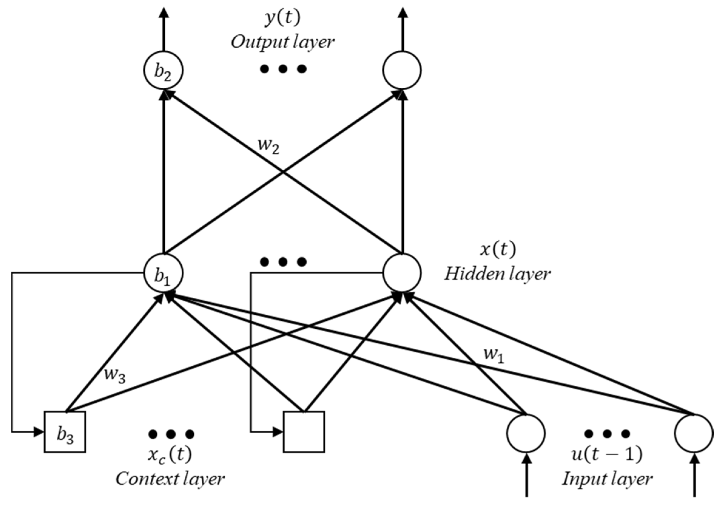
The neural network is an information processing framework and a universal machine learning method with broad applicability in numerous fields. The Elman neural network, which was first introduced by J. L. Elman [35] in 1990, is a well-known local recursion delay feedback neural network, which has a structure similar to the BP network [36], with the addition of a context layer. The schematic representation of the ENN’s architecture can be represented by Figure 1.
The topological structure of ENN typically comprises four distinct layers. The input layer, comprising linear neurons, serves as the entry for external signals and transmits them to the hidden layer. Through the activation function, hidden layer units perform translation or dilation on input signals. Subsequently, the context layer remembers output values from the hidden layer in the previous time step. This layer is used as a one-step delay module to provide a feedback mechanism. Ultimately, the output layer generates the final outputs based on the processed information from previous layers. This structure provides the system with the capacity to handle time-varying characteristics, thereby bolstering network stability and adaptation.
According to the above, assuming the ENN has M inputs and N outputs, and that both the hidden layer and the context layer are set to consist of K layer, the weights from the inputs to the hidden layer, from the hidden layer to the outputs and from the context layer to the hidden layer are represented by w1, w2 and w3, respectively. The thresholds are denoted b1, b2 and b3 for the hidden layer, the output layer and the context layer, respectively. Therefore, the mathematical model is expressed by Formula (1):
x t = f ( w 3 x c t + w 1 u t 1 ) x c t = x t 1 y t = g ( w 2 x t )
In Formula (1), t serves as the current iteration number. u(t − 1) denotes the inputs provided to the ENN during the previous time step. x(t) represents the outputs generated by the hidden layer at t-th step, and the outputs of the context layer are denoted as xc(t). y(t) represents the outputs of ENN at the current time step. The transfer function for the hidden layer and the output layer are denoted as f(∙) and g(∙), respectively.

2.2. Rat Swarm Optimizer

As a meta-heuristic algorithm based on swarm intelligence, the Rat Swarm Optimizer [37] emulates the rat population behavior of chasing and hunting. This algorithm can be summarized in two main parts. The first part involves rats chasing prey through the optimal individual to obtain a better position for searching. The second part is the process by which the rats attack the prey. The mathematical expressions for the two cases are provided in Formula (2), and RSO’s pseudo-algorithm is presented in Algorithm 1.
P t = A X i t + C X b e s t t X i t X i t + 1 = X b e s t t P
In Formula (2), X denotes the position of the rat. t is the current iteration number. Xtbest represents the optimal individual of population during the t-th iteration. Xti signifies the position of i-th rat and Pt is the prey position for Xti. Xit+1 represents the next position of the i-th rat. A and C serve as update coefficients. The coefficient A is calculated by Formula (3):
A = R R t / T
In Formula (3), R and C constrain within [1, 5] and [0, 2], respectively. T is the maximum iteration number.
Algorithm 1 RSO
1Initialization:
2Generate the initial population Xi of the RSO
3Calculate fitness scores and identify X*best
4while tT do
5 for i = 1, 2, …, N do
6 Update parameters using Formula (3)
7 Update population positions using Formula (2)
8 end for
9 Calculate fitness scores and update X*best
10end while

3. Methods

3.1. Improve Algorithm

In this section, a Hyperactivity Rat Swarm Optimizer (HRSO) based on multiple types of chase search and attack actions is proposed to improve the shortcomings of RSO. HRSO implements a two-phase calculation process, comprising a search and a mutation phase. The search phase is further divided into two parts, exploration and exploitation, by means of a nonlinear adaptive parameter. There are five search actions, center point search and cosine search, which are based on the exploration part, and rush search, contrast search and random search, which are based on the exploitation part. The mutation phase employs a stochastic wandering strategy. Algorithm 2 presents the pseudo-algorithm for HRSO.
Algorithm 2 HRSO
1Initialization:
2Generate the initial population Xi of the HRSO
3Calculate fitness scores and identify X*best
4while tT do
5 Execute Search Phase
6 for i = 1, 2, …, N do
7 Update parameters using Formulas (4) and (5)
8 if |E| ≥ 1 then
9 Execute Exploration Search using Algorithm 3
10 elseif |E| < 1 then
11 Execute Exploitation Search using Algorithm 4
12 end if
13 end for
14 Calculate fitness scores and identify X*best
15 Execute Mutation Phase using Algorithm 5
16 Calculate fitness scores and identify X*best
17end while

3.2. Nonlinear Adaptive Parameter

A nonlinear adaptive parameter E is employed to enhance RSO, which is an important parameter to regulate the proportion of exploration and exploitation parts during the search phase. Depending on the absolute value of E, the algorithm either performs exploration part (when |E| ≥ 1) or exploitation part (when |E| < 1). The mathematical expression for E is given as in Formula (4).
E = 2 E 0 c p
In Formula (4), E0 is a random number from –1 to 1. cp is an adaptive parameter that decreases progressively with iterations. Its representation is given as Formula (5):
c p = 1 t / T
According to Formulas (4) and (5), the range of values for parameter E can be determined as −2 to 2.

3.3. Exploration Search

To enable RSO to explore more deeply the invisible domains within search space to improve the efficiency of discovering the global optimal position, center point search and cosine search are introduced in the exploration part of the proposed algorithm.
Center point search is a linear search method based on the average position of the population, which uses cp to control the extended search. This search method is given as Formula (6).
X i t + 1 = c p X i b e s t + r 2 m e a n X i t X b e s t *
In Formula (6), mean(Xti) denotes the average position of the population. r2 constrains within [0, 1].
The cosine search is a search pattern characterized by a wide range of oscillatory variation. A set of adaptive random numbers z is used to control the cosine fluctuation variation. This search method is given as Formula (7).
X i t + 1 = X i b e s t + c p z c o s 2 π r 3 X b e s t * X i t
In Formula (7), the mathematical expression for the parameter z is as follows, in Formula (8):
z = r 5 + r 6
In Formula (8), r3 and r5 are random numbers. r6 is Gaussian distributed random numbers. This is controlled by a random number r4. When r4cp, r6 shows parts greater than 0.5, otherwise, it shows the parts less than 0.5.
To maximize the exploration performance of HRSO, a random number r1, with values between 0 and 1, is used to control the search method. Specifically, if r1 ≥ 0.5, the search iteration is performed using Formula (6), otherwise, Formula (7) is used. The pseudo-algorithm for details of the exploration search is presented in Algorithm 3.
Algorithm 3 Exploration Search
1Update parameters using Formulas (5) and (8)
2Calculate mean(Xti) based on the current population
3when |E| ≥ 1 then
4 if r1 ≥ 0.5 then
5 Update population positions using Formula (6)
6 else then
7 Update population positions using Formula (7)
8 end if
9end when

3.4. Exploitation Search

To enhance the convergence speed and local search capability, three search methods are introduced into the exploitation part of the proposed algorithm, which are rush search, contrast search and random search.
The rush search is the same as the original algorithm, which is Equation (1), but the ranges of the parameters R and C are set to [1, 3] and [–1, 1] respectively, aiming to focus the algorithm on the neighborhood to enhance the local optimization.
The contrast search is performed by randomly selecting two individuals, j1 and j2, from the population and comparing them with the i-th individual, approaching in the direction of the optimal fitness value among the three individuals. The mathematical expression is as in Formulas (9) and (10):
X i t + 1 = X i t + r 7 X i t X j m t
X i t + 1 = X i t + r 7 X j m t X i t
In Formulas (9) and (10), r7 denotes a random number that lies between 0 and 1. m is a constant with the value 1 or 2.
The random search also selects two individuals, with the current individual search in the direction of the optimal fitness value among j1 and j2. It can be expressed by Formulas (11) and (12):
X i t + 1 = X i t + r 8 X j 1 t X j 2 t
X i t + 1 = X i t + r 8 X j 2 t X j 1 t
In Formulas (11) and (12), r8 constrains within [0, 1].
To maximize the exploitation performance of the proposed algorithm, a random constant k is introduced to determine the search methods, where k takes values of 1, 2 and 3. Specifically, k = 1 employs Formula (2) for the rush search, k = 2 utilizes Formula (9) for the contrast search and k = 3 applies Formula (10) for the random search. The pseudo-algorithm for details of the exploitation search is presented in Algorithm 4.
Algorithm 4 Exploitation Search
1.Update random parameters k, j1, and j2
2.when |E| < 1 then
3. if k = 1 then
4. Update population positions using Formula (2)
5. elseif k = 2 then
6. Update random parameters jm
7. if fit(j) < fit(i) then
8. Update population positions using Formula (9)
9. else then
10. Update population positions using Formula (10)
11. end if
12. elseif k = 3 then
13. if fit(j1) < fit(j2) then
14. Update population positions using Formula (11)
15. else then
16. Update population positions using Formula (12)
17. end if
18. end if
19.end when

3.5. Stochastic Wandering Strategy

In the mutation phase, a stochastic wandering strategy is employed to improve the algorithmic capability to jump out of local extreme values. This means that a part of the population is randomly selected to be compared with the global optimization and updated iteratively, and the individual with the best fitness will be retained. This strategy is mathematically expressed as in Formulas (13) and (14):
X i t + 1 = X b e s t * + r a n d n X i t X b e s t *
X i t + 1 = X i t + r 9 X i t X w r o s t * / f i t i f i t w r o s t
In Formulas (13) and (14), randn is a set of normally distributed random numbers. X*wrost denotes the worst individual in a population at the t-th iteration. It is worth noting that a constant NS is used to control the number of individuals selected in this phase, with NS set to 0.2 in this paper. The pseudo-algorithm for details of the mutation phase is presented in Algorithm 5.
Algorithm 5 Mutation Phase
1.for i = 1, 2, …, N do
2. if fit(i) > fit(best) then
3. Update population positions using Formula (13)
4. else fit(i) = fit(best) then
5. Update population positions using Formula (14)
6. end if
7.end for

3.6. Classifier Design

For constructing a complete HRSO-ENNC, the structural design of the hidden layer is also a key factor, indicating that the neuron count of the hidden layer has a significant influence on the ENN’s overall performance. An insufficient number of neurons can cause feature information to be lost during the propagation process, preventing the desired accuracy from being achieved. Conversely, an excessive number of neurons may lead to a more complex system prone to overfitting. It is important to highlight that the configuration of the hidden layer also has effects on the weights and thresholds optimization. Therefore, it is necessary to select a reasonable number for the hidden layer. The method presented in [38] is employed in this research, mathematically formalized as in Formula (15):
K = M + N + a
Formula (15) represents a common empirical equation for determining the number of the hidden layer in neural network, where a represents an integer within the range of [1, 10].
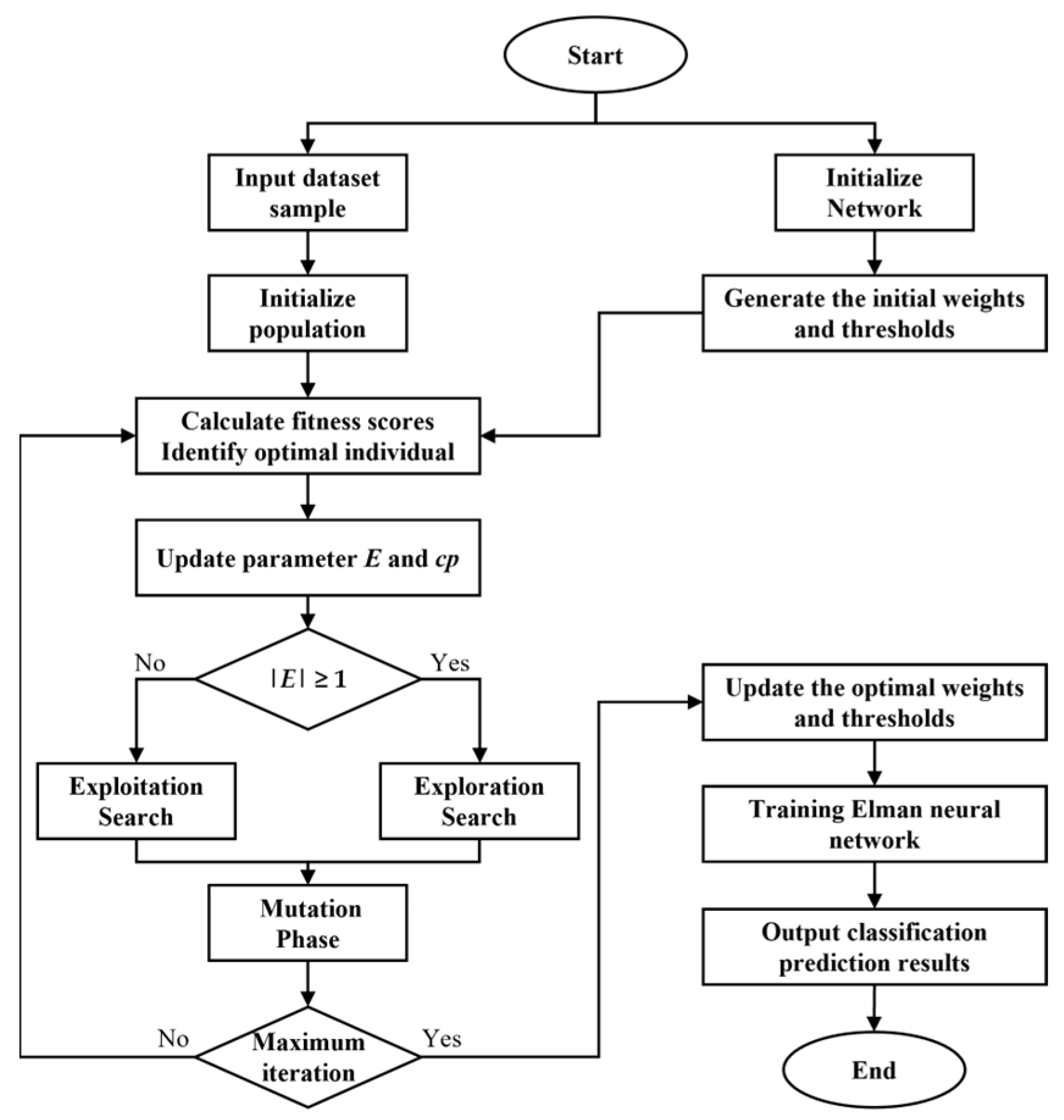
Additionally, the gradient descend method is commonly employed to determine the suitable weights and thresholds in traditional ENN, but it easily obtains a local optimum, ultimately resulting in low accuracy for the system. According to the previous section, the proposed HRSO algorithm ensures an equilibrium between proportions of exploration and exploitation, and it shows a great ability to jump out of the local optimum. In this case, it serves as an adaptive global training method, which means that the proposed algorithm replaces traditional training processes to overcome the shortcomings of the ENN during weights and thresholds optimization. Algorithm 6 presents the pseudo-algorithm for HRSO-ENNC, and Figure 2 represents a specific flowchart.
Algorithm 6 HRSO-ENNC
1.Input: Dataset sample
2.Normalized dataset
3.Selection of training set by the stratified k-fold cross validation method
4.for i = 1, 2, …, k
5. Initialize ENN and HRSO algorithm parameters
6. Calculate fitness scores and identify X*best
7. while tT do
8. Update network parameters using Algorithm 2
9. Calculate fitness scores and identify X*best
10. end while
11. Get X*best for i-th
12. Update network parameters and Training ENN
13. Output classification prediction results
14.end for

4. Experiential Results and Analysis

4.1. Benchmark Functions Test

This section evaluates the HRSO using benchmark functions F1 through F20. F1F7, listed in Table 1, are unimodal functions that are employed to evaluate the algorithm’s performance when there is only one global minimum. F8F13, listed in Table 2, are multimodal functions that are employed to evaluate the algorithm’s performance in searching for a global solution in the case of numerous local minimums. F14F20, listed in Table 3, are fixed-dimension multimodal functions that are employed to evaluate the convergence of the algorithm under low-dimensional problems.
In all of the experiments, the proposed HRSO will be compared with RSO, PSO [39], FA [40], DE [41], BOA [42], WOA [43], GWO [44] and COA [45]. For all of the algorithms employed in this research, the population size is set to 30, and the maximum iteration numbers is set to 500. Each algorithm is independently tested 20 times on the benchmark functions listed in Table 1, Table 2 and Table 3. The results of the test experiments are depicted in Table 4. Among them, the Best, Mean and Std represent the optimal value, arithmetic mean and sample standard deviation, respectively, of results from 20 independent runs of the algorithm. These metrics reflect the algorithm’s theoretical maximum performance, overall average performance and the degree of discretization in outputs.
Experimental results from Table 4 reveal that HRSO exhibits the absolute best performance for F2, F3, F5, and F8–F20. F1 and F4 are both bowl-shaped unimodal functions. For F1, the best result for HRSO is marginally inferior to that for RSO, but it demonstrates superior mean and standard scores. This likely stems from its exceptional performance regarding simple unimodal functions while it is susceptible to local optima. Regarding the more complex F4, as predicted by the F1 results, HRSO outperforms RSO and other algorithms in both best and mean metrics. Although HRSO’s standard deviation on F4 is slightly worse than that of RSO, the difference is marginal. F6 and F7 are smooth and plate-shaped unimodal functions. For these functions, although RSO achieves marginally superior best metric, HRSO attains optimal mean and standard deviation scores across all algorithms, further validating the aforementioned conjecture.
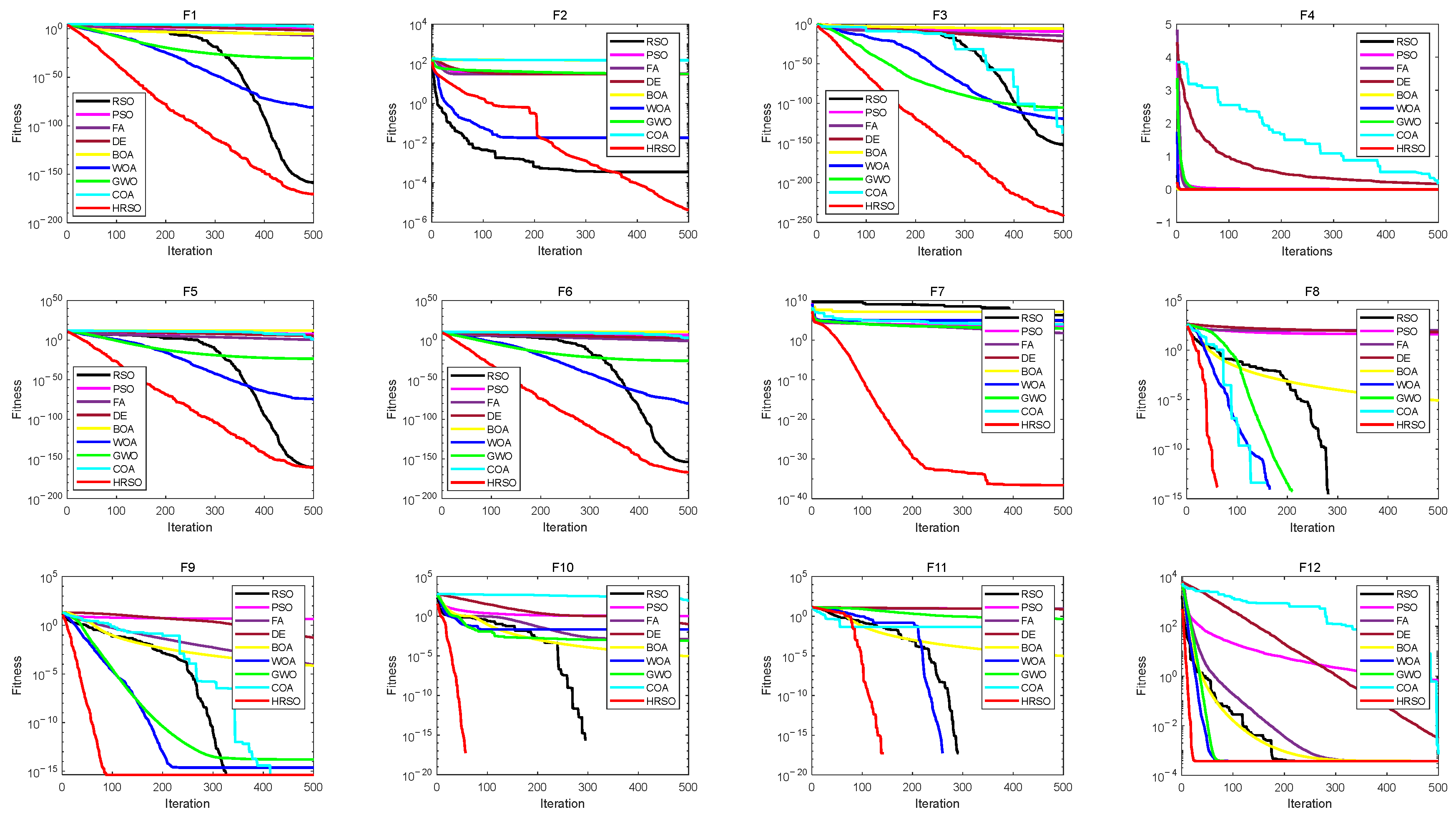
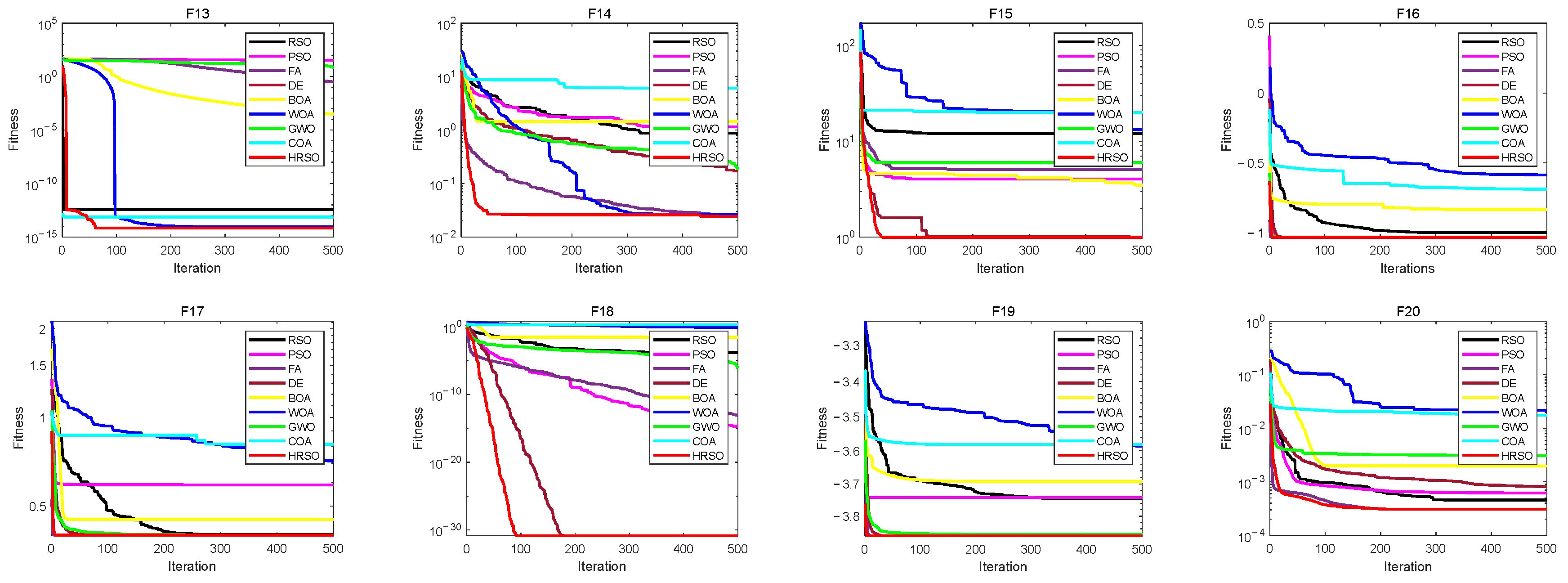
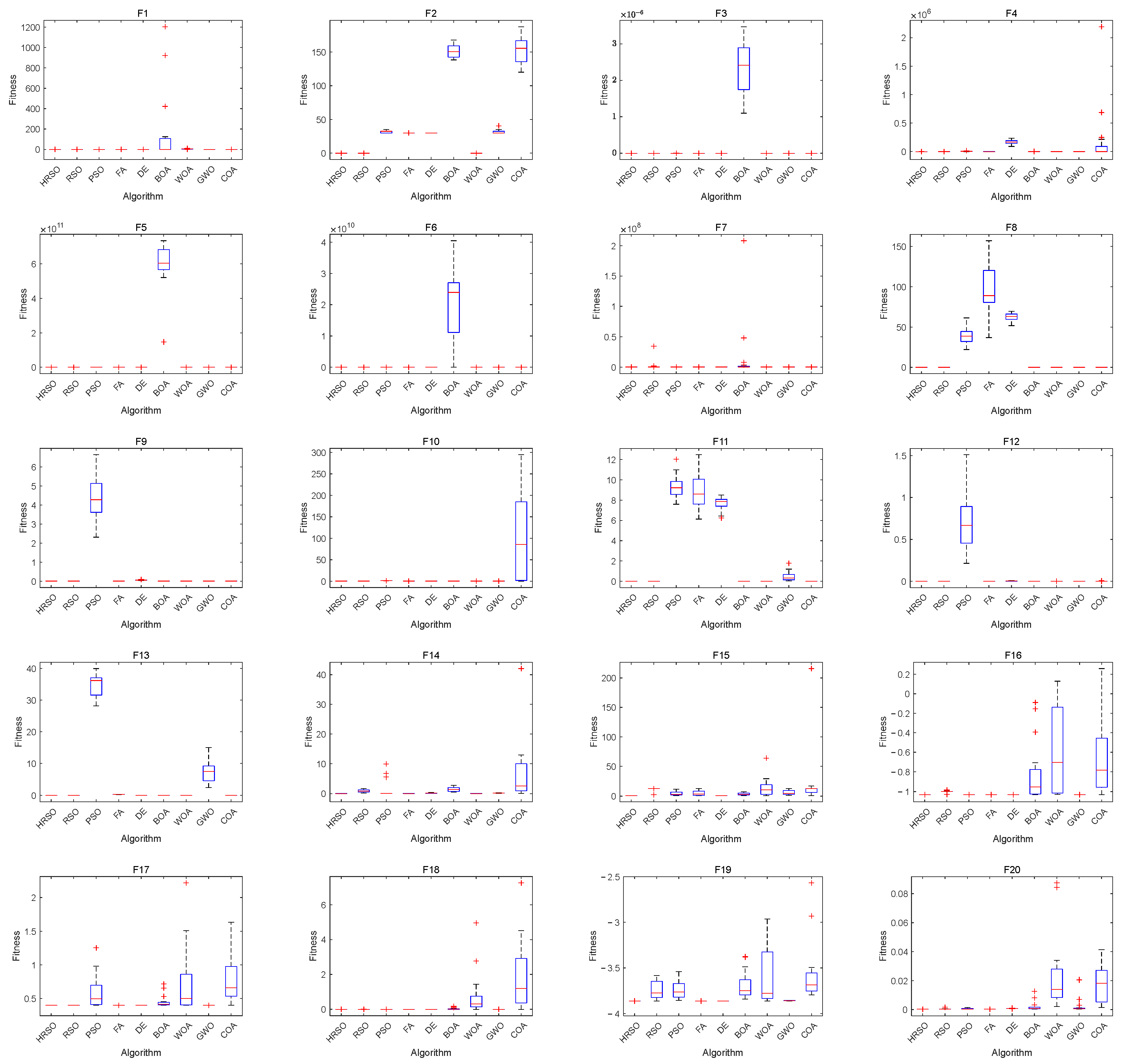
To validate and illustrate the performance of HRSO more intuitively, Figure 3 showcases the convergence curves, Figure 4 presents the boxplots, while Table 5 presents the results of the parameter sensitivity analysis. According to Figure 3 and Figure 4, HRSO exhibits superior performance compared to the other algorithms in both convergence rate and stability, indicating that HRSO is highly exploitable and robust. To further verify the stability of HRSO, Table 5 presents an evaluation of the nonlinear adaptive parameter E, which governs the balance between exploration and exploitation during the search. Using benchmark functions from Table 1, Table 2 and Table 3 and fixing a random number generator seed, experimental results demonstrate that reducing E biases exploitation search and accelerates local convergence, while increasing E shifts toward exploration search and expands global search scope. Notably, the volatility of all of the metrics remained below 2 × 10⁻³, with no statistically significant differences. This further confirms that HRSO exhibits high robustness against variations in the adjustment parameter of E, and even when E is adjusted within a reasonable range, the algorithm maintains stable performance.

4.2. Classification Benchmarks Dataset Test

The classification performance of HRSO-ENNC is analyzed in this part. Additionally, comparative results with RSO-ENNC, PSO-ENNC, FA-ENNC, DE-ENNC, BOA-ENNC, WOA-ENNC, GWO-ENNC and COA-ENNC are provided. The performance is evaluated by seven classic benchmarks for data classification prediction problems. Table 6 provides the dataset name, number of samples, features, classes and distribution of sample quantities across different classes for the seven data classification prediction problems.
In all of the experiments, a stratified seven-fold cross-validation method is utilized to assess the classifier’s performance metrics more accurately. This means that one-seventh of the overall dataset is randomly considered as the test set, while the rest is used for training. Unlike standard cross-validation, the stratified method randomly divides each class into seven equal-sized sets, so that each fold is a better representation of the overall dataset. The classifier is run seven times based on this method, with a different set as the test set each time. The experimental indicators include the values of the maximum, mean and standard deviation for the prediction accuracy on both training and test datasets.
Table 7 and Table 8 present the experimental results of HRSO-ENNC and other algorithm-ENNC for the data classification prediction problem on the training and test dataset, respectively.
Table 7 illustrates that, for the Iris, Balancescale and WBC datasets, the HRSO-ENNC achieves better maximum, mean and standard deviation of the prediction accuracy compared to other algorithm-ENNC on the training dataset. For the remaining datasets, the HRSO-ENNC exhibits better maximum and mean accuracy, with only slightly worse standard deviation compared to DE-ENNC and GWO-ENNC. All observed values are less than 1.07 × 10⁻², but this is not statistically significant and does not indicate that the HRSO-ENNC is unstable.
Similarly to the experiment results on the training dataset, the best testing results are the in Table 8, except for the WBC and Cancer datasets. For these two datasets, the standard deviation score of the HRSO-ENNC is about 1.76 × 10⁻² and 4.50 × 10⁻³ worse than those of the BOA-ENNC and DE-ENNC, respectively. In conclusion, the experimental outcomes reflect that the HRSO overcomes the dependence of the Elman neural network on weights and thresholds, demonstrating the accuracy of its classification performance.

4.3. AlSi10Mg Process Classification Problem

In selective laser melting (SLM), single-track formation critically determines the dimensional accuracy and surface quality of components. Distinct morphological variations may induce defects including internal porosity and poor surface roughness, which can degrade performance. Consequently, effective classification of these morphological features is crucial for ensuring process stability and product quality. An application of process classification is introduced for single-track AlSi10Mg on selective laser melting (SLM) in this section.
The dataset was acquired through orthogonal simulation experiments in which the laser power and scanning speed are equidistant and sampled in the range of 150–250 W and 0.6–1.6 m/s, with multiple repeated trials conducted. Following image sampling, anomalous data are eliminated, resulting in a final dataset of 441 samples. Based on production experience, samples are classified into three distinct morphological categories. In total, 243 normal class samples are continuous and uniform, 145 over-heat class samples are widened and irregular, and 53 no-continuity class samples display a fractured and discontinuous appearance. Seven critical features are extracted via image measurements, including depth, cross-sectional area and effective width, describing melt pool geometry; linear energy density and laser action depth ratio, reflecting energy transfer efficiency; and standard deviation and coefficient of variation, quantifying process fluctuation. These features collectively characterize geometric attributes, energy distribution and process stability to enable precise classification. Table 9 and Table 10 provide specific details of the dataset and feature. Appendix A provides dataset examples across different classes.
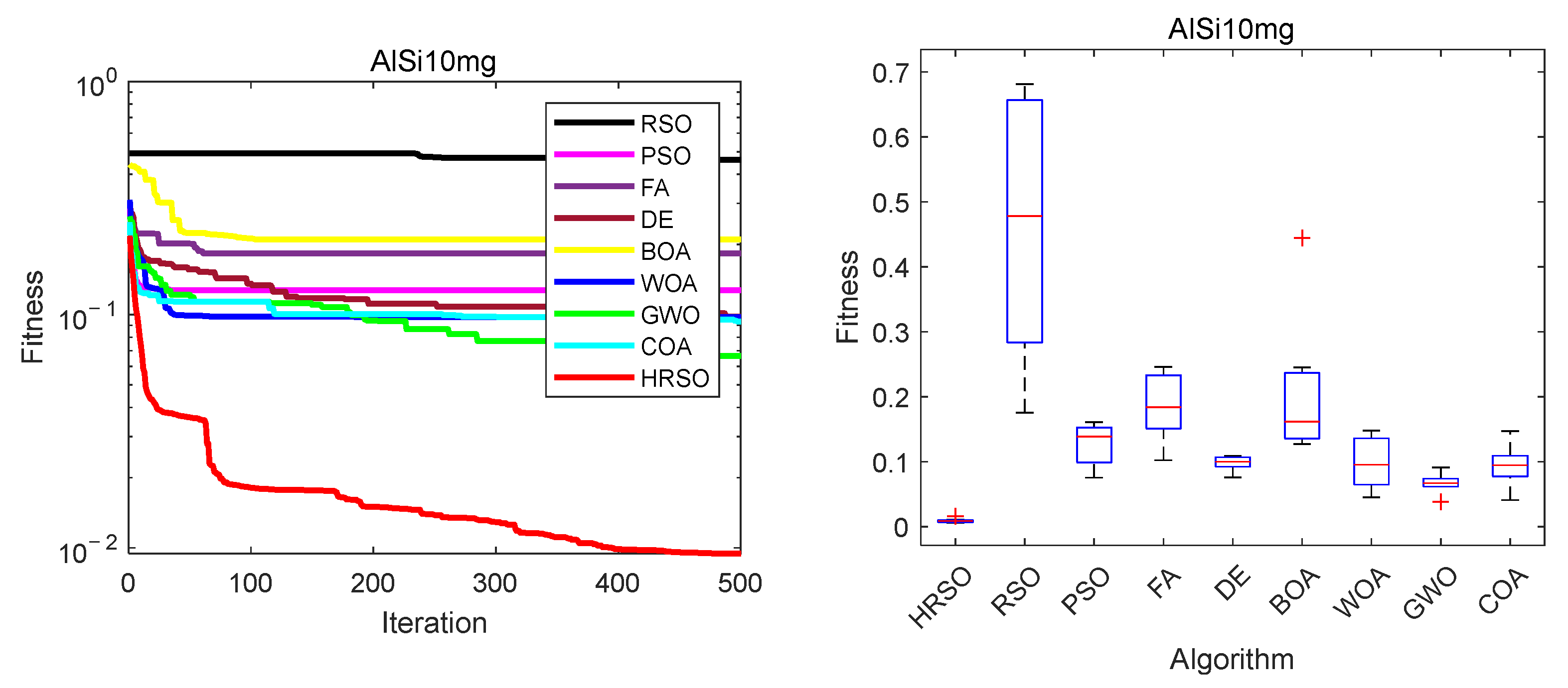
To provide a more objective evaluation of the model’s performance, weighted Precision, weighted Recall and weighted F1-score are included in Table 11 and Table 12. These metrics are calculated as a weighted average using class sample size proportions, effectively mitigating the dominance results of the majority class. Notably, the newly added metrics are the arithmetic means based on the results of the stratified seven-fold cross-validation method. Experimental results presented in Figure 5 confirm that the proposed HRSO-ENNC exhibits superior convergence rate and stability compared to the other classifiers. HRSO-ENNC achieves a maximum identification accuracy of 100%, and on other metrics outperforms all comparison models, as shown in Table 11 and Table 12. This demonstrates the effectiveness and robustness of the HRSO-ENNC in the AlSi10Mg process classification problem.

5. Conclusions

In the current work, we address shortcomings of the Elman neural network (ENN), which easily obtains local optimums and a slow convergence rate. To address the data classification prediction problem, an ENN classifier based on the Hyperactive Rat Swarm Optimizer (HRSO) is proposed. The proposed algorithm is designed as a two-phase calculation process and consists of five search actions. The center point and cosine search significantly enhance the exploration phase of the RSO, while rush, contrast and random search enhance the exploitation phase. Finally, a stochastic wandering strategy is used to jump out of local optimal positions. Experimental results based on benchmark functions confirm that HRSO outperforms other algorithms in both convergence rate and stability. Additionally, the proposed HRSO optimizes the weights and thresholds of ENN to overcome its shortcomings by replacing the traditional training methods. The classification performance of HRSO-ENNC is rigorously evaluated through seven benchmark data classification prediction problems, demonstrating the accuracy and generalizability of the model. Furthermore, HRSO-ENNC achieves a maximum accuracy of 100% in the AlSi10Mg process classification problem, with all other metrics significantly outperforming those of other algorithmic classifiers. The results demonstrate that this classifier is an excellent tool for data classification prediction. Further research has shown that the neural network accumulates more weights and thresholds with an augmented number of inputs and outputs, which makes it difficult for the algorithms to converge. Therefore, subsequent research efforts will prioritize algorithmic enhancements for high-dimensional optimization challenges, thereby improving algorithmic scalability.

Author Contributions

Conceptualization, H.C. and X.L.; methodology, M.H.; software, R.N.; validation, R.N.; formal analysis, Y.X.; investigation, L.S.; resources, H.C.; data curation, Y.X.; writing—original draft preparation, R.N.; writing—review and editing, R.N.; visualization, R.N.; supervision, L.S.; project administration, H.C. and X.L.; funding acquisition, H.C. and X.L. All authors have read and agreed to the published version of the manuscript.

Funding

This research received no external funding.

Data Availability Statement

Data will be made available on request.

Conflicts of Interest

The authors declare no conflicts of interest.

Appendix A

Table A1. Dateset examples across different classes.
DepthCross-Sectional AreaEffective WidthLinear Energy DensityLaser Action Depth RatioStandard DeviationCoefficient of VariationClass
0.03990.00280.06690.25000.63040.07710.1152over-heat
0.03490.00190.05880.21000.65880.05170.0880normal
0.02010.00080.03660.11880.88220.12130.3312no-continuity

References

  1. Kotsiantis, S.B.; Zaharakis, I.D.; Pintelas, P.E. Machine learning: A review of classification and combining techniques. Artif. Intell. Rev. 2006, 26, 159–190. [Google Scholar] [CrossRef]
  2. Sun, D.; Wen, H.; Wang, D.; Xu, J. A random forest model of landslide susceptibility mapping based on hyperparameter optimization using Bayes algorithm. Geomorphology 2020, 362, 107201. [Google Scholar] [CrossRef]
  3. Kuehn, N.M.; Scherbaum, F. A Naive Bayes Classifier for Intensities Using Peak Ground Velocity and Acceleration. Bull. Seismol. Soc. Am. 2010, 100, 3278–3283. [Google Scholar] [CrossRef]
  4. Kovacs, G.; Hajdu, A. Translation Invariance in the Polynomial Kernel Space and Its Applications in KNN Classification. Neural Process. Lett. 2013, 37, 207–233. [Google Scholar] [CrossRef]
  5. Gestel, T.V.; Suykens, J.A.K.; Baesens, B.; Viaene, S.; Vanthienen, J.; Dedene, G.; Moor, D.B.; Vandewalle, J. Benchmarking least squares support vector machine classifiers. Mach. Learn. 2004, 54, 5–32. [Google Scholar] [CrossRef]
  6. Wang, G.C.; Carr, T.R. Marcellus Shale Lithofacies Prediction by Multiclass Neural Network Classification in the Appalachian Basin. Math. Geosci. 2012, 44, 975–1004. [Google Scholar] [CrossRef]
  7. Michie, D.; Spiegelhalter, D.J. Machine Learning, Neural and Statistical Classification. Technometrics 1999, 37, 459. [Google Scholar] [CrossRef]
  8. Zhang, G.P. Neural networks for classification: A survey. IEEE Trans. Syst. Man Cybern. Part C 2000, 30, 451–462. [Google Scholar] [CrossRef]
  9. Sun, J.Y. Learning algorithm and hidden node selection scheme for local coupled feedforward neural network classifier. Neurocomputing 2012, 79, 158–163. [Google Scholar] [CrossRef]
  10. Müller, M.; Stiefel, M.; Bachmann, B.-I.; Britz, D.; Mücklich, F. Overview: Machine Learning for Segmentation and Classification of Complex Steel Microstructures. Metals 2024, 14, 553. [Google Scholar] [CrossRef]
  11. Fang, W.; Huang, J.-X.; Peng, T.-X.; Long, Y.; Yin, F.-X. Machine learning-based performance predictions for steels considering manufacturing process parameters: A review. J. Iron Steel Res. Int. 2024, 31, 1555–1581. [Google Scholar] [CrossRef]
  12. Zhang, L.; Wang, Y.M.; Liu, D.F. Calculating the synthetic efficiency of hydroturbine based on the BP neural network and Elman neural network. Appl. Mech. Mater. 2013, 457–458, 801–805. [Google Scholar] [CrossRef]
  13. Xu, L.; Zhang, Y.T. Quality Prediction Model Based on Novel Elman Neural Network Ensemble. Complexity 2019, 2019, 9852134. [Google Scholar] [CrossRef]
  14. Li, Q.; Qin, Y.; Wang, Z.Y.; Zhao, Z.X.; Zhan, M.H.; Liu, Y. Prediction of Urban Rail Transit Sectional Passenger Flow Based on Elman Neural Network. Appl. Mech. Mater. 2014, 505–506, 1023. [Google Scholar] [CrossRef]
  15. Gong, X.L.; Hu, Z.J.; Zhang, M.L.; Wang, H. Wind Power Forecasting Using Wavelet Decomposition and Elman Neural Network. Adv. Mater. Res. 2013, 608–609, 628–632. [Google Scholar] [CrossRef]
  16. Gupta, T.; Kumar, R. A novel feed-through Elman neural network for predicting the compressive and flexural strengths of eco-friendly jarosite mixed concrete: Design, simulation and a comparative study. Soft Comput. 2024, 28, 399–414. [Google Scholar] [CrossRef]
  17. Wei, L.; Wu, Y.; Fu, H.; Yin, Y. Modeling and Simulation of Gas Emission Based on Recursive Modified Elman Neural Network. Math. Probl. Eng. 2018, 2018, 9013839. [Google Scholar] [CrossRef]
  18. Chiroma, H.; Abdul-Kareem, S.; Ibrahim, U.; Ahmad, I.G.; Garba, A.; Abubakar, A.; Hamza, M.F.; Herawan, T. Malaria Severity Classification Through Jordan-Elman Neural Network Based on Features Extracted from Thick Blood Smear. Neural Netw. World 2015, 25, 565–584. [Google Scholar] [CrossRef]
  19. Boldbaatar, E.A.; Lin, L.Y.; Lin, C.M. Breast Tumor Classification Using Fast Convergence Recurrent Wavelet Elman Neural Networks. Neural Process. Lett. 2019, 50, 2037–2052. [Google Scholar] [CrossRef]
  20. Fu, Q.; Jing, B.; He, P.; Si, S.; Wang, Y. Fault Feature Selection and Diagnosis of Rolling Bearings Based on EEMD and Optimized Elman_AdaBoost Algorithm. IEEE. Sens. J. 2018, 18, 5024–5034. [Google Scholar] [CrossRef]
  21. Arun, C.; Gopikakumari, R. Optimisation of both classifier and fusion based feature set for static American sign language recognition. IET. Image. Process 2020, 14, 2101–2109. [Google Scholar] [CrossRef]
  22. Zhang, M.; Diao, M.; Gao, L.; Liu, L. Neural Networks for Radar Waveform Recognition. Symmetry 2017, 9, 75. [Google Scholar] [CrossRef]
  23. Akarslan, E.; Dogan, R. A novel approach based on a feature selection procedure for residential load identification. Sustain. Energy Grids 2021, 27, 100488. [Google Scholar] [CrossRef]
  24. Chen, D.; Wang, P.; Sun, K.; Tang, Y.; Kong, S.; Fan, J. Simulation and prediction of the temperature field of copper alloys fabricated by selective laser melting. J. Laser Appl. 2022, 34, 042001. [Google Scholar] [CrossRef]
  25. Vaidyaa, P.; John, J.J.; Puviyarasan, M.; Prabhu, T.R.; Prasad, N.E. Wire EDM Parameter Optimization of AlSi10Mg Alloy Processed by Selective Laser Melting. Trans. Indian Inst. Met. 2023, 74, 2869–2885. [Google Scholar] [CrossRef]
  26. Chaudhry, S.; Soulainmani, A. A Comparative Study of Machine Learning Methods for Computational Modeling of the Selective Laser Melting Additive Manufacturing Process. Appl. Sci. 2022, 12, 2324. [Google Scholar] [CrossRef]
  27. Prakash, T.S.; Kumar, A.S.; Durai, C.R.B.; Ashok, S. Enhanced Elman spike Neural network optimized with flamingo search optimization algorithm espoused lung cancer classification from CT images. Biomed. Signal Process. Control 2023, 84, 104948. [Google Scholar] [CrossRef]
  28. Ding, S.; Zhang, Y.; Chen, J.; Jia, W. Research on using genetic algorithms to optimize Elman neural networks. Neural Comput. Appl. 2013, 23, 293–297. [Google Scholar] [CrossRef]
  29. Wang, X.F.; Liang, C.C.; Jiang, J.G.; Ju, L.L. Sensor Compensation Based on Adaptive Ant Colony Neural Networks. Adv. Mater. Res. 2011, 301–303, 876–880. [Google Scholar] [CrossRef]
  30. Barile, C.; Casavola, C.; Pappalettera, G.; Kannan, V.P.; Mpoyi, D.K. Acoustic Emission and Deep Learning for the Classification of the Mechanical Behavior of AlSi10Mg AM-SLM Specimens. Appl. Sci. 2022, 13, 189. [Google Scholar] [CrossRef]
  31. Barile, C.; Casavola, C.; Pappalettera, G.; Kannan, V.P. Damage Progress Classification in AlSi10Mg SLM Specimens by Convolutional Neural Network and k-Fold Cross Validation. Materials 2022, 15, 4428. [Google Scholar] [CrossRef]
  32. Ji, Z.; Han, Q.Q. A novel image feature descriptor for SLM spattering pattern classification using a consumable camera. Int. J. Adv. Manuf. Technol. 2020, 110, 2955–2976. [Google Scholar] [CrossRef]
  33. Li, J.; Cao, L.; Xu, J.; Wang, S.; Zhou, Q. In situ porosity intelligent classification of selective laser melting based on coaxial monitoring and image processing. Measurement 2022, 187, 110232. [Google Scholar] [CrossRef]
  34. Moghadam, A.T.; Aghahadi, M. Adaptive Rat Swarm Optimization for Optimum Tuning of SVC and PSS in a Power System. Int. Trans. Electr. Energy Syst. 2022, 2022, 4798029. [Google Scholar] [CrossRef]
  35. Elman, J.L. Finding Structure in Time. Cogn. Sci. 1990, 14, 179–211. [Google Scholar] [CrossRef]
  36. Rumelhart, D.E.; Hinton, G.E.; Williams, R.J. Learning Representations by Back-Propagating Errors. Nature 1986, 323, 533–536. [Google Scholar] [CrossRef]
  37. Dhiman, G.; Garg, M.; Nagar, A.; Kumar, V.; Dehghani, M. A novel algorithm for global optimization: Rat swarm optimizer. J. Amb. Intel. Hum. Comp 2021, 12, 8457–8482. [Google Scholar] [CrossRef]
  38. Ye, S. RMB exchange rate forecast approach based on BP neural network. Phys. Scr. 2012, 33, 287–293. [Google Scholar] [CrossRef]
  39. Khare, A.; Rangnekar, S. A review of particle swarm optimization and its applications in Solar Photovoltaic system. Appl. Soft Comput. 2013, 13, 2997–3006. [Google Scholar] [CrossRef]
  40. Kumar, V.; Kumar, D. A Systematic Review on Firefly Algorithm: Past, Present, and Future. Arch. Comput. Methods Eng. 2021, 28, 3269–3291. [Google Scholar] [CrossRef]
  41. Slowik, A.; Kwasnicka, H. Evolutionary algorithms and their applications to engineering problems. Neural Comput. Appl. 2020, 32, 12363–12379. [Google Scholar] [CrossRef]
  42. Arora, S.; Singh, S. Butterfly optimization algorithm: A novel approach for global optimization. Soft Comput. 2018, 23, 715–734. [Google Scholar] [CrossRef]
  43. Mirjalili, S.; Lewis, A. The Whale Optimization Algorithm. Adv. Eng. Softw. 2016, 95, 51–67. [Google Scholar] [CrossRef]
  44. Mirjalili, S.; Mirjalili, S.M.; Lewis, A. Grey Wolf Optimizer. Adv. Eng. Softw. 2014, 69, 46–61. [Google Scholar] [CrossRef]
  45. Zhang, Q.; Bu, X.; Zhan, Z.-H.; Li, J.; Zhang, H. An efficient Optimization State-based Coyote Optimization Algorithm and its applications. Appl. Soft Comput. 2023, 147, 110827. [Google Scholar] [CrossRef]
Figure 1. Architecture diagram of Elman neural network.
Processes 13 02802 g001
Figure 2. The flowchart of HRSO-ENNC.
Processes 13 02802 g002
Figure 3. Convergence graphs of HRSO, RSO, PSO, FA, DE, BOA, WOA, GWO and COA.
Processes 13 02802 g003aProcesses 13 02802 g003b
Figure 4. Boxplot of HRSO, RSO, PSO, FA, DE, BOA, WOA, GWO and COA.
Processes 13 02802 g004
Figure 5. Convergence graphs and boxplots of HRSO, RSO, PSO, FA, DE, BOA, WOA, GWO and COA.
Processes 13 02802 g005
Table 1. Expression of F1F7 Benchmark Function.
FunctionFunction FormulaDimRangeFbest
F1: Sphere i = 1 n x i 2 30−100, 1000
F2: Lunacek’s Bi-Sphere m i n i = 1 n x i u 1 2 ,   d · n + s · i = 1 n x i u 2 2 30−10, 100
F3: Sum of Different Powers i = 1 n x i i + 1 30−1, 10
F4: Trid i = 1 n x i 1 2 i = 2 n x i x i 1 30−n2, n2−4930
F5: Bent Cigar x 1 2 + 10 6 i = 2 n x i 2 30−100, 1000
F6: High Conditioned Elliptic i = 1 n 10 6 i 1 n 1 x i 2 30−100, 1000
F7: Zakharov i = 1 n x i 2 + i = 1 n 0.5 x i 2 + i = 1 n 0.5 x i 4 30−100, 1000
Table 2. Expression of F8F13 Benchmark Function.
FunctionFunction FormulaDimRangeFbest
F8: Generalized Rastrigin i = 1 n x i 2 10 c o s 2 π x i + 10 30−5.12, 5.120
F9: Ackley 20 e x p 0.2 1 n i = 1 n x i 2 e x p 1 n i = 1 n cos 2 π x i + 20 + e 30−32, 320
F10: Generalized Griewank 1 4000 i = 1 n x i 2 + i = 1 n cos x i i + 1 30−600, 6000
F11: Schaffer g x 1 , x 2 + g x 2 , x 3 + + g x n 1 , x n + g x n , x 1
g x , y = 0.5 + s i n 2 x 2 + y 2 0.5 ( 1 + 0.001 x 2 + y 2 ) 2
30−100, 1000
F12: Modified Schwefel 418.9829 × n i = 1 n g z i
g z i = z i s i n z i 1 / 2 i f   z i 500   500 y i 1 s i n 500 y i 1 z i 500 2 10,000 n i f   z i > 500 y i 2 500 s i n y i 2 500 z i + 500 2 10,000 n i f   z i < 500
z i = x i + 4.209687462275036 E + 02
y i 1 = m o d z i , 500       y i 2 = m o d z i , 500
30−100, 1000
F13: Weierstrass i = 1 n k = 0 20 0.5 k c o s 2 · 3 k π x i + 0.5 n k = 0 20 0.5 k c o s 3 k π 30−100, 1000
Table 3. Expression of F14F20 Benchmark Function.
FunctionFunction FormulaDimRangeFbest
F14: Bukin 100 x 2 0.01 x 1 2 + 0.01 x 1 + 10 2−15, 30
F15: Shekel’s Foxholes 1 500 + j = 1 25 1 j + i = 1 2 x i a i j 6 1 2−65.53, 65.531
F16: Six-Hump Camel-Back 4 x 1 2 2.1 x 1 4 + 1 3 x 1 6 + x 1 x 2 4 x 2 2 + 4 x 2 4 2−5, 5−1.031
F17: Branin x 2 5.1 4 π 2 x 1 2 + 5 π x 1 6 2 + 10 1 1 8 π c o s x 1 + 10 2−5, 150.398
F18: Levy s i n 2 3 π x 1 + x 1 1 2 1 + s i n 2 3 π x 2 + x 2 1 2 1 + s i n 2 2 π x 2 2−10, 100
F19: Hartman’s Family i = 1 4 c i e x p j = 1 3 a i j x j p i j 2 31, 3−3.86
F20: Kowalik i = 1 11 a i x 1 b i 2 + b i x 2 b i 2 + b i x 3 + x 4 2 4−5, 53 × 10−4
Table 4. Experimental Results for Benchmark Function.
FunctionIndexHRSORSOPSOFADEBOAWOAGWOCOA
F1Best3.63 × 10−1921.23 × 10−2042.551.02 × 10−71.19 × 10−26.97 × 10−63.50 × 10−973.06 × 10−329.84 × 10⁻¹⁹
Mean4.75 × 10−1712.03 × 10−1595.431.47 × 10−72.38 × 10−27.74 × 10−61.20 × 10−815.09 × 10−311.46 × 10²
Std0.001.61 × 10−1581.882.09 × 10−89.73 × 10−34.75 × 10−75.37 × 10−817.53 × 10−313.32 × 10²
F2Best1.42 × 10−79.49 × 10−73.00 × 1013.00 × 1013.00 × 1011.38 × 1011.20 × 10−43.00 × 1011.20 × 102
Mean4.09 × 10−63.52 × 10−43.20 × 1013.00 × 1013.00 × 1011.52 × 1021.84 × 10−23.16 × 1011.53 × 102
Std7.08 × 10−68.16 × 10−42.073.73 × 10−111.19 × 10−59.661.77 × 10−23.002.10 × 101
F3Best5.75 × 10−2623.87 × 10−2061.90 × 10−113.16 × 10−163.17 × 10−231.10 × 10−63.09 × 10−1564.72 × 10−1184.73 × 10−136
Mean9.58 × 10−2436.20 × 10−1535.67 × 10−102.31 × 10−152.39 × 10−222.34 × 10−67.19 × 10−1209.58 × 10−1062.36 × 10−127
Std0.002.77 × 10−1521.03 × 10−91.68 × 10−152.07 × 10−226.88 × 10−73.21 × 10−1193.64 × 10−1051.06 × 10−126
F4Best4.82 × 103−1.21 × 1031.95 × 102−4.44 × 1038.91 × 1041.93 × 101−1.45 × 10³−2.61 × 1023.00 × 101
Mean−4.21 × 10³−9.20 × 1024.19 × 103−2.54 × 1031.68 × 1053.19 × 101−1.07 × 10³−1.41 × 1021.76 × 105
Std1.74 × 1021.23 × 1023.57 × 1031.15 × 1034.03 × 1045.854.61 × 1027.54 × 1015.03 × 105
F5Best5.61 × 10−1975.61 × 10−1871.19 × 1071.306.33 × 1041.47 × 10113.83 × 10−901.19 × 10−253.94 × 10⁻⁷
Mean9.91 × 10−1625.02 × 10−1614.58 × 1071.491.44 × 1056.02 × 10112.54 × 10−752.49 × 10−241.55 × 101
Std4.36 × 10−1612.22 × 10−1602.49 × 1071.98 × 10−16.41 × 1041.27 × 10111.13 × 10−743.71 × 10−246.07 × 101
F6Best1.18 × 10−1901.28 × 10−1942.80 × 1053.83 × 10−29.18 × 1016.12 × 1042.87 × 10−906.50 × 10−291.25 × 10⁻³
Mean1.05 × 10−1671.30 × 10−1541.89 × 1065.68 × 10−21.60 × 1022.05 × 10101.36 × 10−806.19 × 10−275.50 × 10²
Std0.005.64 × 10−1541.38 × 10−21.38 × 10−25.18 × 1011.03 × 10104.94 × 10−801.40 × 10−261.82 × 10³
F7Best3.29 × 10−1281.13 × 10−1804.97 × 1021.06 × 10−25.83 × 1041.43 × 1013.65 × 1037.87 × 10−42.08 × 10⁻²⁰
Mean2.79 × 10−471.87 × 1061.89 × 1035.67 × 1017.58 × 1041.35 × 1078.67 × 1048.47 × 1029.33 × 103
Std1.25 × 10−467.67 × 1061.38 × 1038.90 × 1018.24 × 1034.71 × 1072.51 × 1041.35 × 1033.03 × 104
F8Best0.000.002.19 × 1013.68 × 1015.17 × 1017.40 × 10−60.000.000.00
Mean0.000.003.82 × 1019.52 × 1016.24 × 1017.91 × 10−60.000.000.00
Std0.000.009.923.12 × 1015.193.75 × 10−70.000.000.00
F9Best4.44 × 10−164.44 × 10−162.307.36 × 10−53.52 × 10−26.61 × 10−54.44 × 10−161.11 × 10−144.44 × 10⁻¹⁶
Mean4.44 × 10−164.44 × 10−164.418.82 × 10−55.42 × 10−27.07 × 10−52.40 × 10−151.70 × 10−144.44 × 10⁻¹⁶
Std0.000.001.048.05 × 10−61.55 × 10−22.73 × 10−62.15 × 10−153.51 × 10−150.00
F10Best0.000.009.37 × 10−11.89 × 10−74.32 × 10−28.02 × 10−60.000.000.00
Mean0.000.001.031.36 × 10−39.75 × 10−28.70 × 10−62.06 × 10−28.24 × 10−49.41 × 101
Std0.000.003.52 × 10−23.34 × 10−33.38 × 10−24.16 × 10−79.22 × 10−22.54 × 10−39.59 × 101
F11Best0.000.007.596.126.248.89 × 10−60.002.09 × 10−20.00
Mean0.000.009.368.877.709.76 × 10−60.004.73 × 10−10.00
Std0.000.001.091.575.96 × 10−15.77 × 10−70.004.59 × 10−10.00
F12Best3.82 × 10−43.82 × 10−42.14 × 10−13.82 × 10−42.08 × 10−33.82 × 10−43.82 × 10−43.82 × 10−43.82 × 10−4
Mean3.82 × 10−43.82 × 10−46.80 × 10−13.82 × 10−43.08 × 10−33.82 × 10−43.82 × 10−43.82 × 10−47.13 × 10−4
Std0.000.003.08 × 10−12.94 × 10−97.64 × 10−41.75 × 10−84.07 × 10−130.001.41 × 10−3
F13Best7.11 × 10−153.77 × 10−132.81 × 1012.74 × 10−19.13 × 10−152.28 × 10−41.42 × 10−142.524.97 × 10−14
Mean7.11 × 10−153.77 × 10−133.47 × 1013.19 × 10−19.24 × 10−153.12 × 10−49.24 × 10−147.307.53 × 10−14
Std0.000.003.562.28 × 10−29.25 × 10−154.13 × 10−59.25 × 10−143.281.84 × 10−14
F14Best1.01 × 10−32.35 × 10−15.00 × 10−28.27 × 10−33.63 × 10−25.02 × 10−15.52 × 10−36.93 × 10−21.24 × 10−1
Mean2.44 × 10−28.81 × 10−11.152.50 × 10−21.72 × 10−11.442.69 × 10−21.83 × 10−16.08
Std1.30 × 10−24.34 × 10−12.791.65 × 10−21.05 × 10−17.19 × 10−11.56 × 10−26.05 × 10−29.48
F15Best9.98 × 10−12.339.98 × 10−19.98 × 10−19.98 × 10−19.98 × 10−19.98 × 10−11.131.03
Mean9.98 × 10−11.22 × 1014.055.119.98 × 10−13.491.32 × 1015.992.00 × 101
Std0.002.312.994.240.001.911.45 × 1013.724.63 × 101
F16Best−1.03−1.03−1.03−1.03−1.03−1.03−1.03−1.03−1.03
Mean−1.03−1.00−1.03−1.03−1.03−8.33 × 10⁻¹−5.86 × 10⁻¹−1.03−6.87 × 10⁻¹
Std1.25 × 10−168.00 × 10−32.04 × 10−169.72 × 10−152.22 × 10−162.88 × 10−14.42 × 10−15.22 × 10−83.54 × 10−1
F17Best3.98 × 10−13.98 × 10−13.98 × 10−13.98 × 10−13.98 × 10−13.99 × 10−13.98 × 10−13.98 × 10−14.00 × 10−1
Mean3.98 × 10−14.00 × 10−15.89 × 10−13.98 × 10−13.98 × 10−14.45 × 10−17.12 × 10−13.98 × 10−18.11 × 10−1
Std0.002.08 × 10−32.27 × 10−11.01 × 10−140.008.66 × 10−24.77 × 10−16.33 × 10−73.85 × 10⁻¹
F18Best1.35 × 10−318.12 × 10−81.55 × 10−211.84 × 10−151.35 × 10−312.61 × 10−42.29 × 10−173.79 × 10−84.46 × 10−4
Mean1.35 × 10−311.56 × 10−42.02 × 10−157.51 × 10−141.35 × 10−312.68 × 10−27.39 × 10−17.19 × 10−71.80
Std0.003.13 × 10−47.13 × 10−156.47 × 10−143.52 × 10−474.92 × 10−21.196.85 × 10−71.89
F19Best−3.86−3.86−3.86−3.86−3.86−3.84−3.86−3.86−3.80
Mean−3.86−3.74−3.74−3.86−3.86−3.69−3.59−3.86−3.58
Std1.79 × 10−158.40 × 10−29.10 × 10−27.75 × 10−152.28 × 10−151.42 × 10−13.50 × 10−12.68 × 10−33.04 × 10−1
F20Best3.07 × 10−43.09 × 10−43.07 × 10−43.07 × 10−44.84 × 10−43.28 × 10−42.25 × 10−33.44 × 10−41.40 × 10−3
Mean3.07 × 10−44.58 × 10−46.17 × 10−43.07 × 10−48.05 × 10−41.98 × 10−32.18 × 10−23.06 × 10−31.75 × 10−2
Std2.28 × 10−142.97 × 10−45.41 × 10−44.20 × 10−141.28 × 10−43.04 × 10−32.40 × 10−26.16 × 10−31.31 × 10⁻²
Table 5. Experimental Results for Parameter Sensitivity Analysis.
FunctionIndexE [−1, −1]E [−2, −2]E [−3, −3]
F2Best2.67 × 10−72.39 × 10−52.84 × 10−5
Mean2.07 × 10−74.11 × 10−67.75 × 10−6
Std2.68 × 10−73.48 × 10−53.87 × 10−5
F13Best7.11 × 10−152.82 × 10−131.34 × 10⁻¹³
Mean7.11 × 10−157.11 × 10−150.00
Std7.11 × 10−157.11 × 10−150.00
F14Best1.53 × 10−24.83 × 10−21.56 × 10−2
Mean3.02 × 10−32.28 × 10−21.56 × 10−2
Std5.99 × 10−32.55 × 10−21.36 × 10−2
Table 6. Classification Prediction Benchmarks Dataset.
NumberDatasetSamplesFeatureClassesDistribution
1Iris1504350, 50, 50
2Wine17813359, 71, 48
3Balance-scale6254349, 288, 288
4Seeds2107370, 70, 70
5WBC68392444, 239
6Jain37322276, 97
7Cancer68392444, 239
Table 7. Classification Accuracy for Training Dataset.
DatasetValuesHRSO-ENNCRSO-ENNCPSO-ENNCFA-ENNCDE-ENNCBOA-ENNCWOA-ENNCGWO-ENNCCOA-ENNC
IrisMax100.00%89.84%96.90%95.31%96.12%85.94%97.67%98.45%95.35%
Mean98.33%82.00%88.79%87.23%92.78%80.45%90.55%96.44%80.67%
Std0.01670.05430.10200.04600.02220.10100.05730.01980.1180
WineMax99.34%79.61%93.42%91.45%84.87%90.07%87.50%97.67%89.54%
Mean96.73%71.01%81.17%76.04%83.34%84.66%82.31%94.60%80.72%
Std0.02260.07960.07080.07170.01490.04740.06340.02290.0480
BalanceMax94.03%69.40%88.97%71.96%83.40%80.97%88.62%92.35%88.06%
scaleMean90.53%58.61%79.07%66.59%80.37%74.88%84.59%89.73%79.39%
Std0.01180.06120.05120.04090.02330.03260.04210.01500.0569
SeedsMax97.22%88.89%87.22%87.22%90.56%86.11%93.33%96.67%93.33%
Mean95.40%79.60%92.78%77.78%88.25%75.63%89.29%94.98%89.05%
Std0.01670.08460.08540.05130.01410.07680.03040.01100.0371
WBCMax97.78%97.09%97.61%96.08%97.61%97.44%97.26%97.78%96.42%
Mean97.34%95.73%93.09%93.90%96.22%95.83%96.00%97.04%94.56%
Std0.00350.01760.03540.01480.00650.01250.01040.00360.0205
JainMax99.69%94.67%96.55%94.69%95.92%95.94%96.87%96.55%95.94%
Mean97.50%92.58%94.82%93.79%95.35%94.01%95.71%95.63%92.81%
Std0.01520.02850.01010.01570.00450.03630.01500.01170.0204
CancerMax98.63%95.56%97.27%96.24%96.92%97.10%96.92%97.63%96.75%
Mean97.80%93.51%95.10%94.34%96.17%95.78%95.71%97.19%95.36%
Std0.00680.01780.01770.01110.00360.01640.01910.00350.0167
Table 8. Classification Accuracy for Testing Dataset.
DatasetValuesHRSO-ENNCRSO-ENNCPSO-ENNCFA-ENNCDE-ENNCBOA-ENNCWOA-ENNCGWO-ENNCCOA-ENNC
IrisMax100.00%90.48%95.24%100.00%100.00%95.24%100.00%100.00%90.48%
Mean93.35%79.99%80.77%86.73%90.69%74.61%88.59%92.22%76.56%
Std0.05530.07850.09690.07980.07350.12000.11800.05930.1010
WineMax96.15%73.08%92.00%96.15%87.50%96.15%92.00%95.58%84.62%
Mean93.21%64.49%78.69%70.69%80.41%80.76%71.88%90.81%75.16%
Std0.01680.08840.07930.01310.04870.10800.02870.03610.0852
BalanceMax91.01%71.91%88.89%75.56%82.22%77.53%86.52%89.43%85.39%
scaleMean88.00%58.09%79.02%66.07%77.75%70.56%82.41%87.75%79.51%
Std0.01260.07640.05850.05910.04020.04850.03480.02610.0535
SeedsMax100.00%90.00%90.00%90.00%93.33%86.67%96.67%100.00%96.67%
Mean92.38%77.62%82.86%75.24%86.19%75.71%88.57%91.82%86.67%
Std0.04950.07280.07440.07100.06530.07130.05390.06100.0903
WBCMax98.98%96.94%98.98%93.88%98.98%95.92%98.98%98.98%98.98%
Mean95.75%93.41%94.44%92.82%94.72%93.85%95.02%95.47%93.41%
Std0.03090.03270.03820.02070.03550.01330.02460.01760.0350
JainMax100.00%98.11%98.11%98.15%96.30%98.11%96.30%100.00%100.00%
Mean97.31%92.26%92.22%93.01%93.58%93.58%94.63%95.49%92.23%
Std0.01730.03850.03560.03150.02380.03340.01730.03310.0383
CancerMax97.96%94.90%96.94%97.96%95.92%97.96%97.96%97.96%97.96%
Mean96.48%92.97%93.85%94.13%95.15%95.76%94.29%96.02%94.28%
Std0.01330.01400.01970.02750.00880.02410.03870.01420.0341
Table 9. Single-track AlSi10Mg classification problem.
DatasetSamplesFeatureClassesDistribution
AlSi10Mg44173145, 243, 53
Table 10. Detailed description of dataset features.
FeaturePhysical MeaningRangeUnit
depthrepresents the measured depth of the melt pool0.0529, 0.0128mm
cross-sectional arearepresents the measured area of the melt pool0.0047, 0.0004mm2
effective widthrepresents effective melt pool transverse width0.0793, 0.0223mm
linear energy densityrepresents the energy delivered by laser per unit length0.4167,0.0938J/mm
laser action depth ratiorepresents laser powder melting efficiency0.9813, 0.5065unitless
standard deviationrepresents the dispersion of melt pool width0.1839, 0.0218unitless
coefficient of variationrepresents the stability of melt pool processing0.7653, 0.0159unitless
Table 11. AlSi10Mg Process Classification Accuracy for Training Dataset.
DatasetValuesHRSO-ENNCRSO-ENNCPSO-ENNCFA-ENNCDE-ENNCBOA-ENNCWOA-ENNCGWO-ENNCCOA-ENNC
AlSi10MgMax100%87.37%94.96%96.02%94.69%95.23%97.88%97.35%96.30%
Mean99.24%76.71%89.72%88.56%92.67%91.66%93.63%95.77%93.47%
Std0.00430.09640.03150.04170.01200.02930.04730.01680.0323
Weighted P
(Mean)
98.93%77.26%82.94%86.25%93.79%89.71%92.98%96.68%91.69%
Weighted R
(Mean)
98.90%80.11%89.83%89.42%93.25%89.84%94.18%96.45%92.71%
Weighted F1
(Mean)
0.98890.77050.86030.87200.93260.88700.93100.96430.9124
Table 12. AlSi10Mg Process Classification Accuracy for Testing Dataset.
DatasetValuesHRSO-ENNCRSO-ENNCPSO-ENNCFA-ENNCDE-ENNCBOA-ENNCWOA-ENNCGWO-ENNCCOA-ENNC
AlSi10MgMax100%86.89%92.19%92.06%98.44%96.88%98.44%100%98.41%
Mean98.40%75.81%87.97%87.49%92.07%90.87%92.42%94.34%93.62%
Std0.01330.11100.03240.03760.03260.04490.05810.03540.0367
Weighted P
(Mean)
97.42%74.94%81.43%83.06%92.96%84.84%87.28%95.93%93.80%
Weighted R
(Mean)
97.29%75.66%87.99%87.33%91.85%88.64%91.17%95.52%92.96%
Weighted F1
(Mean)
0.97260.71510.84250.84570.91760.86060.88850.95500.9296
Disclaimer/Publisher’s Note: The statements, opinions and data contained in all publications are solely those of the individual author(s) and contributor(s) and not of MDPI and/or the editor(s). MDPI and/or the editor(s) disclaim responsibility for any injury to people or property resulting from any ideas, methods, instructions or products referred to in the content.