Application of an Automated Machine Learning-Driven Grid Block Classification Framework to a Realistic Deep Saline Aquifer Model for Accelerating Numerical Simulations of CO₂ Geological Storage

Abstract

Numerical simulations are essential for optimizing CO₂ geological storage in deep saline aquifers; however, their substantial computational demands pose a significant challenge. This study introduces an automated machine learning (ML)-driven grid block classification framework applied to a realistic deep saline aquifer model to accelerate numerical simulations while maintaining accuracy. The methodology employs an ML and interquartile range-based classifier to distinguish grid blocks as either fast- or slow-varying. ML-based proxy models are applied exclusively to slow-varying regions, while traditional iterative methods handle dynamic, fast-varying regions. Results confirm a considerable reduction in computational costs without compromising predictive accuracy. Validated under realistic reservoir conditions, the approach demonstrates scalability and robustness, supporting efficient, accurate large-scale CO₂ storage simulations and advancing sustainable subsurface sequestration strategies.

1. Introduction

Global warming is widely acknowledged as one of the most urgent challenges facing humanity, with carbon dioxide (CO₂) emissions identified as a primary contributor [1]. Between 1990 and 2015, anthropogenic CO₂ emissions have shown a significant upward trend, increasing by nearly 60% [2]. This rise is evident in atmospheric CO₂ levels, which are projected to reach 429.6 parts per million (ppm) by May 2025—the highest concentration in over 2 million years [3]. To combat climate change, carbon capture and storage (CCS) has emerged as one of the most promising technologies, with research suggesting that its full implementation could reduce global emissions by 20% by 2050 and up to 55% by the end of the century [4].

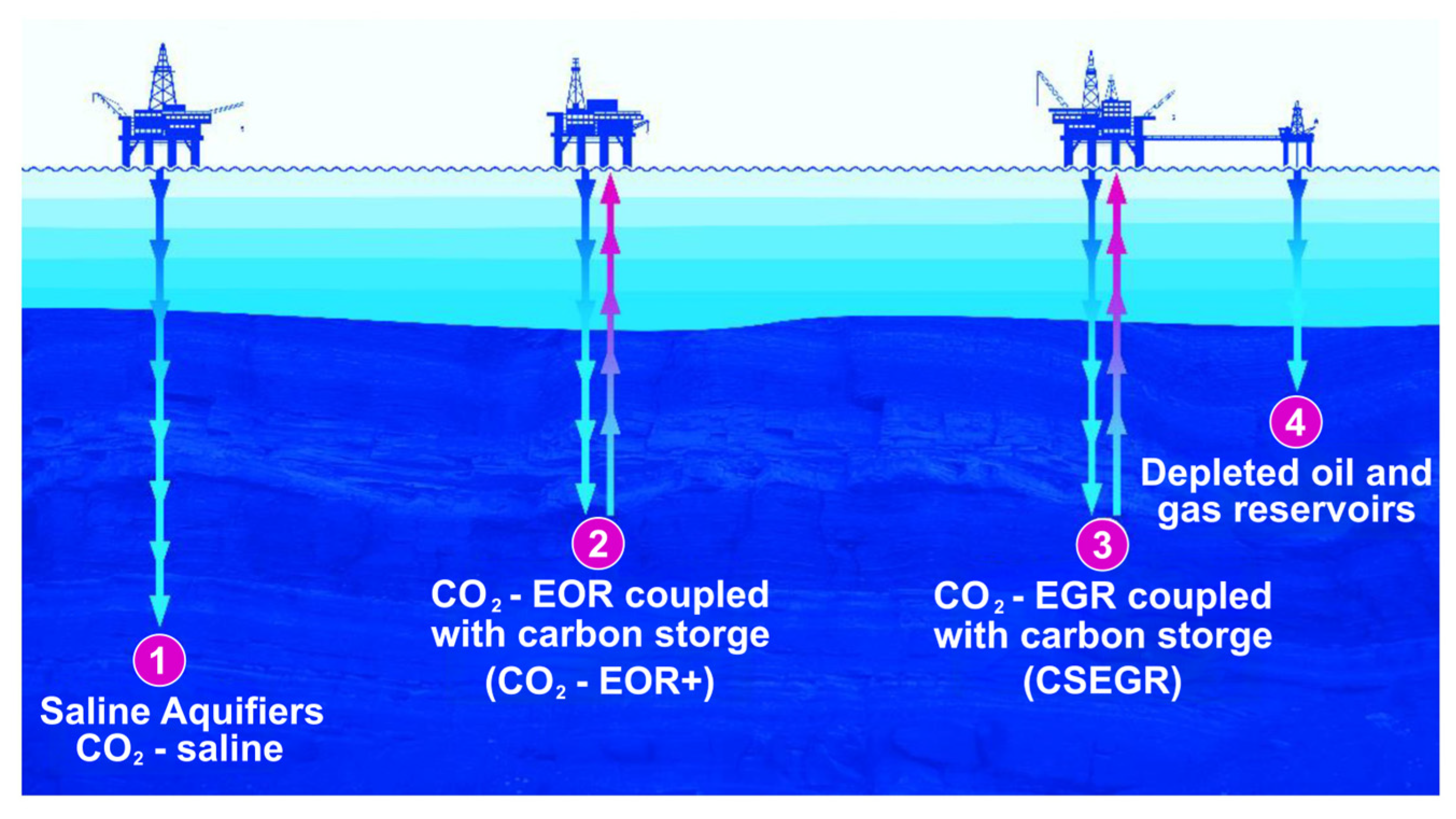
A critical component of CCS is the secure and permanent storage of captured CO₂, which is achieved through geological storage in subsurface porous formations. As illustrated in Figure 1, available geological storage options include deep saline aquifers [5], mature oil and gas reservoirs [6,7] where tertiary recovery methods are applied to stimulate additional production—known as Enhanced Oil Recovery (EOR) and Enhanced Gas Recovery (EGR), respectively—and depleted oil and gas reservoirs [8] that are no longer economically viable for hydrocarbon production. Among these options, saline aquifers exhibit the greatest storage potential, offering several key advantages such as stable storage, strong feasibility, high reservoir porosity and permeability, and large storage capacity [9].

The standard procedure for storing CO₂ in saline aquifers involves injecting it in a supercritical state at depths greater than 800 m [10]. In this state, CO₂ has a higher density than its gaseous form but lower density and viscosity than the surrounding brine [11,12]. Long-term storage is governed by four primary trapping mechanisms, as shown in Figure 2. Structural trapping occurs when CO₂ accumulates beneath impermeable caprock within structural and stratigraphic traps [10]. Solubility trapping involves the partial dissolution of CO₂ into the formation brine [10], while mineral trapping results from dissolved CO₂ reacting with metal cations to form stable carbonate minerals [10]. Finally, residual gas trapping immobilizes CO₂ within pore spaces at irreducible gas saturation [10].

The conventional approach to optimizing CO₂ storage strategies relies on numerical simulations, which enable engineers to predict and manage CO₂ plume migration and pressure distribution within brine-bearing geological formations. These simulations play a critical role in ensuring the secure containment of injected CO₂ by evaluating various injection scenarios and assessing potential risks such as overpressure, caprock integrity failure, and fault reactivation. Through continuous monitoring and analysis, engineers can implement optimized injection strategies that mitigate the risks of leakage, induced seismicity, and CO₂ and formation brine displacement into water-supply aquifers, thereby enhancing the long-term stability of CO₂ storage sites. However, the computational demands of these simulations, particularly those employing Equations of State (EoS) [13], can be substantial.

Proxy models, also known as surrogate models or metamodels [14], offer a computationally efficient alternative for optimizing CO₂ injection strategies. These models, represented by the function $\mathbf{y}=\mathbf{f}\left(\mathbf{x}\right)$, where $\mathbf{x}$ represents input parameters (e.g., well location, initial conditions, injection schedules) and $\mathbf{y}$ represents the reservoir response, can rapidly generate predictions that closely approximate the results of high-fidelity reservoir simulations within acceptable error bounds. Unlike traditional simulation methods requiring iterative solutions, proxy models, once developed, can be directly evaluated for any given reservoir configuration, enabling rapid assessments of potential outcomes.

A specific subcategory of proxy models is smart proxy models, first introduced by Mohaghegh et al. [15]. These are trained using machine learning (ML) and pattern recognition techniques to approximate high-fidelity models. Within this category, grid-based smart proxy models enable grid-level prediction of dynamic reservoir properties—such as pressure and phase saturations—at any time.

Extensive research has established the efficacy of grid-based smart proxy models in accurately replicating high-resolution reservoir simulation outputs. For instance, in 2012, Mohaghegh et al. [16] applied this methodology to three distinct case studies: a giant oil field in the Middle East, a CO₂ sequestration project in Australia, and a numerical simulation study of a potential carbon storage site in the United States. In the same year, Gholami and Mohaghegh [17] further demonstrated the adaptability of this approach by employing a grid-based smart proxy model to simulate CO₂ sequestration in a saline formation in Illinois.

Subsequent research has continued to explore the potential of grid-based smart proxy modeling, particularly for CO₂ sequestration applications. In 2014, Shahkarami et al. [18] developed a model for the SACROC unit, successfully predicting pressure behavior and phase saturation distributions over time. Amini et al. [19] applied a similar methodology to a CO₂ sequestration project in Australia, reinforcing its applicability in large-scale storage simulations. In 2017, Alenezi and Mohaghegh [20] expanded the application of smart proxy modeling to both the grid block and well levels in a study of the SACROC unit in Scurry County, Texas. More recently, Gholami et al. [21] developed a coupled grid-based and well-based smart proxy model for the same unit.

In 2024, Kanakaki et al. [22] introduced a novel ML-driven approach to enhance the efficiency of grid-based smart proxy models for CO₂ sequestration in deep saline aquifers. Their methodology addresses the computational challenges of large-scale reservoir modeling by introducing a classification framework that distinguishes between fast-varying and slow-varying grid blocks. This classification optimizes computational resource allocation, ensuring high accuracy in regions with significant pressure and CO₂ saturation changes while employing grid-based proxies in more stable areas.

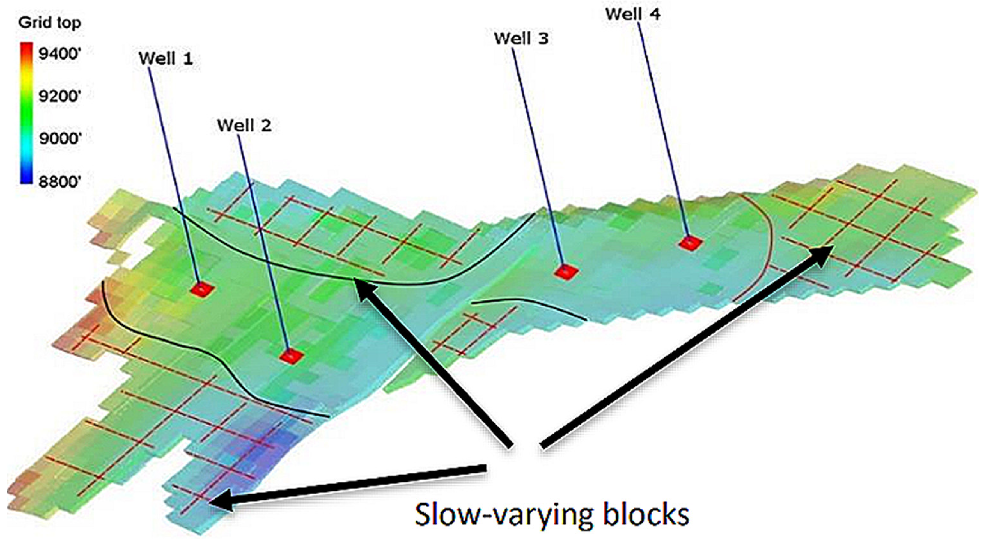
The approach consists of two key stages. In the first stage, an automated ML-based classifier, combined with interquartile range (IQR) analysis, systematically identifies fast- and slow-varying grid blocks, minimizing operator dependency and ensuring consistency across different simulation scenarios. Fast-varying grid blocks typically correspond to regions near injection and production wells, where pressure and saturation exhibit significant fluctuations. In contrast, slow-varying grid blocks are found in areas farther from wells (Figure 3) or in post-injection phases, where CO₂ migration is governed predominantly by capillary and gravitational forces.

In the second stage, ML models predict the state of slow-varying grid blocks based on the temporal evolution of their neighboring cells, leveraging their gradual changes to enhance computational efficiency. Meanwhile, conventional iterative methods are applied exclusively to fast-varying cells to preserve numerical accuracy in dynamically evolving regions. By significantly reducing the number of equations requiring full numerical solution, this hybrid methodology achieves substantial acceleration in reservoir simulations while maintaining predictive reliability.

In this study, we extend the methodology proposed in [22] by applying their framework to a real world reservoir, as opposed to the simplified box-model reservoir used in their original work. By transitioning from an idealized representation to a more complex and geologically realistic reservoir, we aim to assess the practical viability of their approach. Specifically, this application seeks to evaluate the accuracy and computational efficiency of the framework in a real-world context. This step is critical for validating the scalability and robustness of the methodology, ensuring its applicability to field-scale CO₂ sequestration projects.

By demonstrating the feasibility and effectiveness of the ML-based framework in a realistic reservoir setting, this work contributes to advancing CO₂ storage technologies. The findings highlight the potential for more precise and efficient evaluations of candidate storage sites and injection strategies, thereby addressing critical challenges in sustainable subsurface CO₂ sequestration.

The structure of this paper is as follows: Section 2 provides an overview of the methodology, Section 3 presents the case study, Section 4 discusses the results, and Section 5 concludes with key findings and implications.

2. Methodology

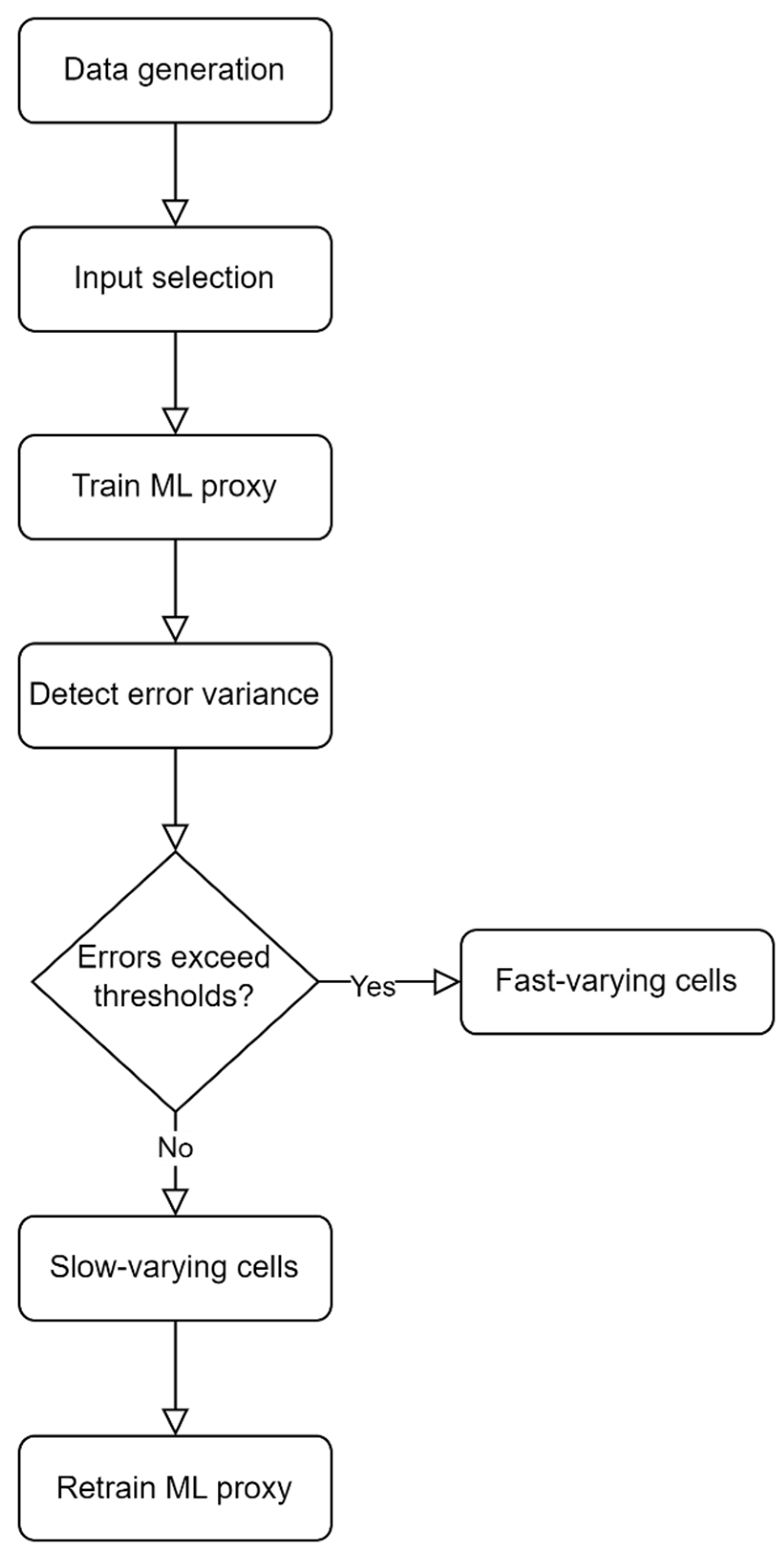
The workflow, illustrated in Figure 4, outlines the machine learning (ML)-driven grid block classification and proxy modeling framework, detailing the sequential steps from automated grid clustering to ML-based prediction of the slow-varying regions within a reservoir model. The process begins with a full-physics reservoir simulator that generates high-fidelity time-series data, including pressure and fluid saturation profiles across all grid blocks. These datasets form the foundation for developing, training, and validating grid-based proxy models capable of capturing the intricate spatial and temporal dynamics of the reservoir system. By doing so, the framework enables accurate prediction of future reservoir states.

At the core of the proxy model is a nonlinear mapping that relates the past states of a target grid cell and of its neighbors to the target cell’s future state, thus capturing the complex interdependencies and spatiotemporal dynamics inherent in reservoir systems. As outlined in

Table 1. Input space.

Feature	Description	Role in ML Model
$dP/dt$	Temporal rate of change in pressure at the focal grid block and its neighbors over time intervals $t_{i-2}$ to $t_{i-1}$ and $t_{i-1}$ to $t_i$.	Captures the temporal dynamics and system evolution.
$dS/dt$	Temporal rate of change in saturation at the focal grid block and its neighbors over time intervals $t_{i-2}$ to $t_{i-1}$ and $t_{i-1}$ to $t_i$.	Reflects fluid movement and its temporal progression.
$P_i$	Pressure at the focal grid block and neighboring cells at $t_i$.	Provides the current pressure state of the reservoir.
$S_i$	Saturation at the focal grid block and neighboring cells at $t_i$.	Indicates the current distribution of fluid phases.

, the input space includes key variables such as the rates of change in pressure $dP/dt$ and saturation $dS/dt$ for both the focal grid block and its adjacent cells, calculated over two consecutive time intervals: from $t_{i-2}$ to $t_{i-1}$ and from $t_{i-1}$ to $t_i$. Since the simulator outputs $P$ and $S$ only at discrete time points, analytic derivatives, demanded by the governing differential equations that the simulator solves, cannot be obtained; instead, numerical derivatives serve as the sole means for estimating the pressure and saturation rates. In the slow-variation regime targeted by this framework, where pressure and saturation evolve smoothly, these numerical derivatives closely approximate the analytical ones; significant divergence arises only during rapid transients or when time intervals become excessively large, both of which fall outside the model’s intended operating envelope.

An important advantage of using derivatives, rather than relying solely on raw pressure and saturation values, is their inherent time step invariance. This property ensures that the proxy model remains independent of specific time intervals, allowing it to integrate with the solver’s adaptive time-stepping algorithm. This design preserves the model’s robustness and flexibility, ensuring that predictions are not tied to a rigid time grid but instead reflect the intrinsic dynamics of the reservoir. Additionally, the use of derivatives as inputs is grounded in the principles of the Taylor series expansion, which provides a mathematical framework for approximating time-varying functions. By using derivatives computed across two consecutive intervals, the methodology implicitly captures information analogous to the second derivative. Specifically, the rate of change from $t_{i-2}$ to $t_{i-1}$ and from $t_{i-1}$ to $t_i$ reflects not only the current slope (first derivative) but also the temporal evolution of these rates of change.

In addition to the derivative-based features, the input dataset also incorporates the current pressure and saturation states at $t_i$ for both the focal grid block and its immediate neighbors, thereby encoding spatial-derivative information. These values provide a snapshot of the reservoir’s most recent state, serving as a baseline for predicting the system’s immediate future state. By combining current states with their rates of change, the model effectively balances short-term trends with real-time information, enhancing predictive accuracy.

The reason why only the first shell of neighbors is used is that, although the full-physics solver mathematically ties every cell to all others, under slow-variation conditions only the first neighbor shell exerts a meaningful influence on the focal cell. Restricting the proxy model’s inputs to each focal cell and its immediate neighbors, therefore, captures the essential pressure–saturation couplings while disregarding negligible far-field effects, preserving accuracy and dramatically reducing computational complexity.

Once the ML model is trained, it outputs the predicted rates of change in pressure and saturation ($dP/dt$ and $dS/dt$) for the focal cell between $t_i$ and $t_{i+1}$, enabling the prediction of future reservoir behavior. In practice, however, blocks undergoing rapid transients produce large errors because the neural network cannot fully learn their fast dynamics, whereas more steady, slow-varying blocks remain predictable. To handle this, the workflow unfolds in two stages: first, every grid block is labeled fast- or slow-varying based on its ML prediction error, and second, only the slow-varying blocks are used to train the proxy, with fast-varying blocks handed off to the full-physics solver.

To distinguish the slow regimes from the fast ones, prediction errors across all grid blocks and time steps are analyzed via an interquartile range (IQR)-based statistical method, which calculates error variance for each grid block. IQR is determined as the difference between the third quartile ($Q3$) and the first quartile ($Q1$) of the error distribution. Grid blocks with errors falling outside the range defined by $Q1-k\times IQR$ (lower threshold) or $Q3+k\times IQR$ (upper threshold) are classified as fast-varying, while those within this range are deemed as slow-varying (Figure 5). The sensitivity of this classification is controlled by a hyperparameter, $k$, which adjusts the thresholds. A lower value of $k$ narrows the IQR bounds, flagging more blocks as fast-varying and, thus, necessitating additional high-fidelity calculations—thereby increasing computational demand. Conversely, a higher $k$ widens the bounds, reducing the number of fast-varying blocks requiring full-physics solves and optimizing computational efficiency. This adaptive approach ensures that the model balances accuracy and computational cost, making it suitable for large-scale reservoir simulations.

In the second stage, grid blocks classified as outliers in pressure, saturation predictions, or both are excluded from proxy model development and redirected to the conventional iterative nonlinear solver. The remaining slow-varying blocks are then used to train the ML proxy. In this workflow, both “Train ML proxy” and “Retrain ML proxy” in Figure 4 denote the same three-layer feedforward ANN. The term “Retrain” emphasizes that, after classification, the proxy is reapplied only to the slow-varying subset to generate state predictions, while the fast-varying cells are passed to the numerical simulator. This division optimizes computational efficiency: the much faster ML proxy handles the majority of grid blocks with low spatial and temporal variance, while the more resource-intensive nonlinear solver handles exclusively on the fast-varying blocks.

The framework originally proposed by Kanakaki et al. [22] was limited to predicting the state of interior focal cells only, that is the cells with six adjacent faces. In this paper, the framework has been extended to address a significant challenge: the development of a single grid-based proxy model capable of handling multiple types of cells, particularly given the distinct characteristics of interior and boundary grid blocks within a reservoir model. A key distinction between these grid block types lies in the number of neighboring cells. Interior grid blocks are fully connected, usually experiencing fluid flow across all six faces as they are in direct contact with six adjacent cells. In contrast, boundary grid blocks have fewer neighboring cells, typically five or fewer, due to their location at the edges of the reservoir or adjacent to geological features. This reduced connectivity, combined with no-flow or constant-pressure boundary conditions, often leads to simpler behavior and more predictable pressure and saturation profiles.

To overcome this challenge, boundary cells are treated as analogous to interior cells through the introduction of imaginary cells. This approach extends the applicability of the ML model by enabling it to account for boundary effects without requiring separate models for different grid block types. The imaginary cell is defined by assigning adjusted properties to simulate interior-like conditions. For example, its pressure is set equal to the focal boundary cell’s pressure, mimicking a no-flow boundary condition where no pressure gradient exists in the direction of the imaginary cell. Similarly, its saturation is matched to the focal cell, ensuring consistency in how cells with five or six neighbors are handled. This adjustment allows the model to generalize across both interior and boundary grid blocks, improving its robustness and predictive accuracy.

It is important to note that this study focuses specifically on boundary cells with five neighbors, as they constitute the majority of boundary cells in the reservoir model. Figure 6 illustrates how boundary cells are adjusted to resemble interior cells through the introduction of an imaginary cell. On the left, the green block represents a boundary focal cell with five neighbors (in transparent white grid). On the right, the imaginary cell (purple, dotted grid) is added to ensure consistent treatment of boundary and interior grid blocks in the proxy model.

3. Case Study Description

To demonstrate the algorithm’s ability to distinguish regions with rapid temporal variations from those exhibiting slower changes, while accurately predicting the state of the latter, a three-dimensional (3D) reservoir model was developed to generate the required spatiotemporal dataset. This model simulates a deep saline aquifer and is designed to numerically replicate the dynamics of CO₂ injection and brine production under realistic geological and operational conditions.

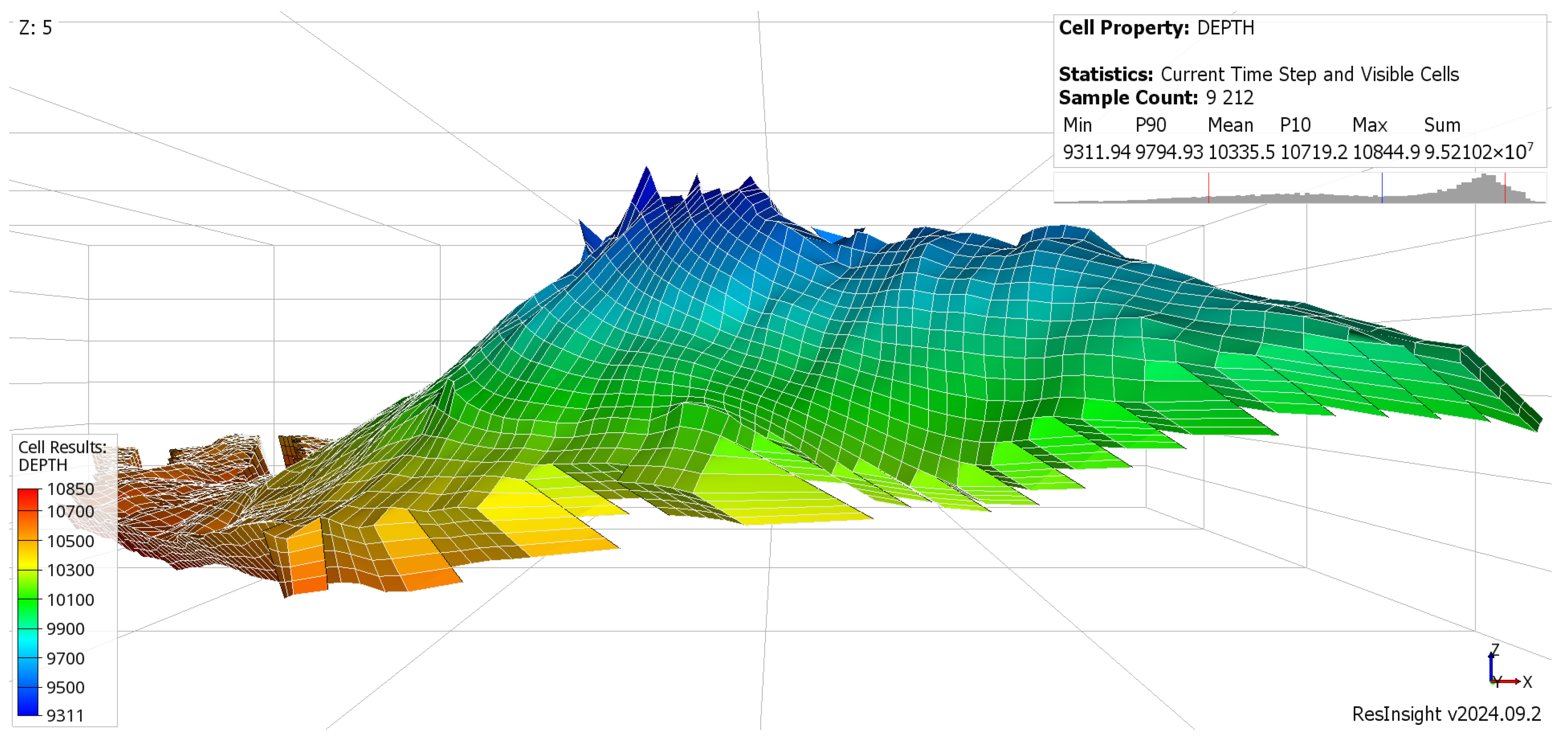
The reservoir grid was constructed using corner-point geometry and consists of 120 × 163 × 4 cells in the X, Y, and Z directions, respectively, resulting in a total of 78,240 grid cells. Of these, 9212 cells are active and represent the geological features of the modeled aquifer, capturing its structural complexity and stratigraphic heterogeneity. The remaining cells are inactive, corresponding to zero-porosity reservoir volumes that delineate non-flow zones such as boundaries or regions outside the aquifer’s active area. These cells are excluded from the flow solution arrays during the memory- and time-intensive simulation stages.

The aquifer’s inclined structural profile is shown in Figure 7. Near its crest, the reservoir forms a steep slope resembling an anticline, that is a geological formation characterized by upward-arching rock layers that create a dome-like structure. Anticlinal traps are particularly important during carbon storage operations, as they play a key role in confining the buoyant CO₂ plume. Upon injection, the CO₂, being less dense than the surrounding brine, rises due to buoyant forces and spreads laterally until it encounters the anticline. There, the plume becomes trapped beneath the impermeable cap rock at the crest of the structure. While the CO₂ is physically confined within the anticline, the pressure induced by the injection propagates through the interconnected pore spaces of the reservoir rock, impacting areas far beyond the immediate extent of the CO₂ plume.

The aquifer is characterized by a relatively simple geological structure, with no apparent faulting or fracturing, and it is tightly sealed by shale formations. With a bulk volume of 2.4 × 10¹¹ ft³ and an initial water in place of 1.7 × 10⁹ STB, the reservoir demonstrates significant storage capacity. Additionally, it exhibits a salinity of approximately 65,000 ppm and a temperature of 200 °F, consistent with geothermal gradients typical of its depth.

Figure 8 provides valuable insights into the reservoir’s fluid flow characteristics, revealing its anisotropic and heterogeneous nature. In the horizontal plane, permeability in the X- and Y-directions is identical, with a P90 of 91 mD, a mean of 272 mD, and a P10 of 572 mD, confirming the presence of extensive high-quality lateral flow pathways. In contrast, vertical permeability (PERMZ) is an order of magnitude lower (P90 = 18 mD, mean = 54 mD, P10 = 114 mD), reflecting typical anisotropy caused by features such as shale barriers, laminations, or depositional characteristics that restrict vertical flow. This anisotropic behavior, expressed as $k_X=k_Y\gg k_Z$, underscores the dominance of lateral flow in the reservoir.

Porosity within the reservoir grid is uniformly set to 0.25 across all cells. This uniform porosity indicates a consistent storage capacity throughout the reservoir. The contrast between heterogeneous permeability and uniform porosity highlights the reservoir’s dual characteristics, which involves complex flow dynamics balanced by stable and predictable storage capacity. The reservoir’s characteristics are summarized in

Table 2. Aquifer characteristics.

Parameter	Value
Average depth (ft)	10,340
Temperature (°F)	200
Salinity (ppm)	65,000
Average horizontal permeability (mD)	272
Average vertical permeability (mD)	55
Porosity	0.25
Bulk volume (ft3)	2.4 × 1011
Water in place (STB)	1.7 × 109

.

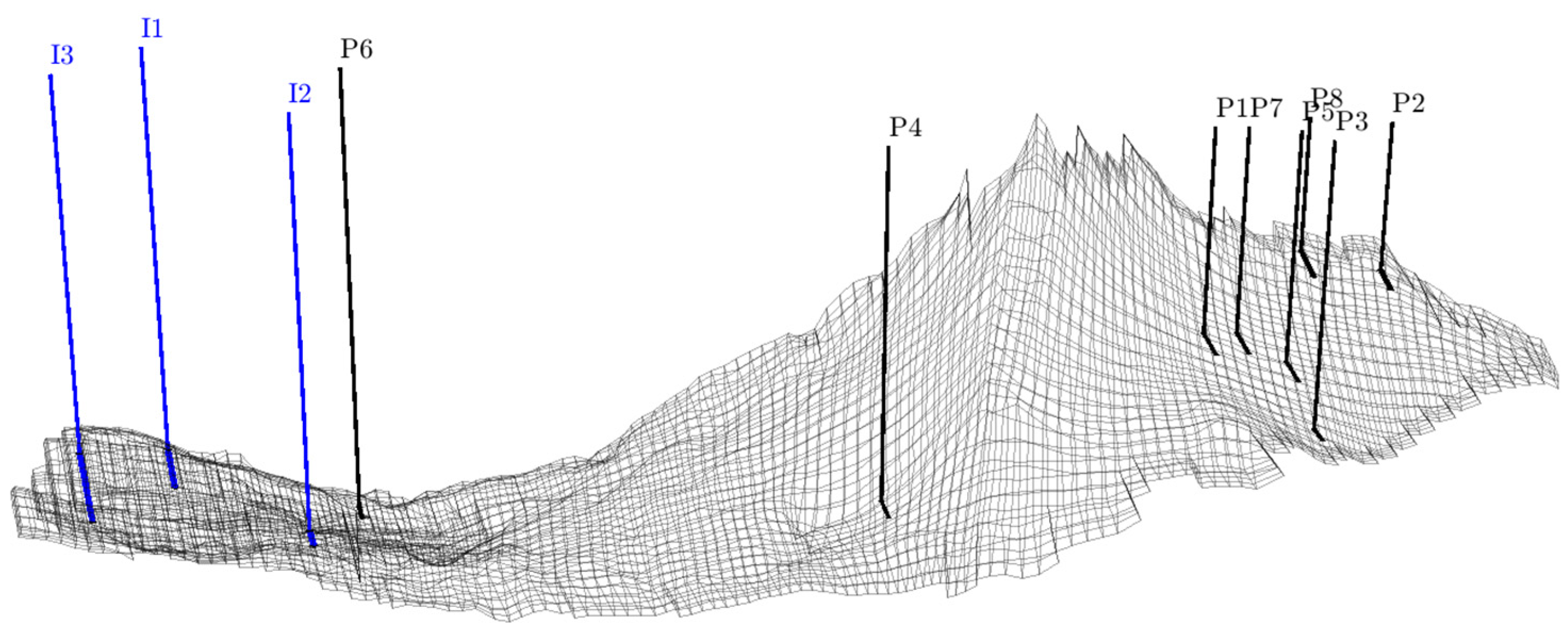
To optimize storage efficiency, three vertical and fully penetrating injection wells (I1, I2, and I3) were strategically positioned in the downdip region of the modeled aquifer, as shown in Figure 9. This placement, informed by the reservoir’s structural inclination and permeability anisotropy, promotes the controlled upward migration of injected CO₂. At the same time, it ensures progressive utilization of the reservoir’s capacity as the CO₂ plume migrates, thereby maximizing its long-term storage potential.

Figure 10 depicts the initial pressure distribution within the reservoir, with an average reservoir pressure of 5151 psi, indicating a slightly overpressurized aquifer. To manage pressure and optimize CO₂ injection, eight brine production wells (P1 to P8) were strategically placed within the aquifer. The majority of these producers are positioned on the opposing side of the crest, while producers P6 and P4 are placed at key positions to maintain pressure and control CO₂ plume migration. Producer P6, located along the anticipated path of the CO₂ plume, acts as a pressure sink due to its strategic position. Producer P4 is positioned to ensure uniform plume migration despite the gravitational pressure differential, which causes the CO₂ to migrate unevenly toward the crest. By moderating pressure in its vicinity, P4 facilitates even plume advancement by the end of the CCS period.

The aquifer model’s operational strategy is further defined by a set of production and injection constraints aimed at maintaining reservoir integrity and ensuring long-term CO₂ storage efficiency. At the field level, the production capacity is regulated with a maximum brine production rate of 77,000 barrels per day and a gas rate limit of 6000 Mscf per day. These constraints are enforced across the entire field and the designated production group, ensuring a balanced withdrawal of reservoir fluids to accommodate the injected CO₂. Simultaneously, gas injection is carefully managed with a field-wide and group-level maximum injection rate of 170,000 Mscf per day, designed to stabilize reservoir pressures while supporting controlled plume migration.

At the well level, the eight production wells are operated with individual constraints to maintain optimal reservoir performance. Each well is capped with a maximum brine production rate of 55,000 barrels per day and a gas production limit of 4000 Mscf per day, alongside a bottom-hole pressure limit of 3000 psi. These parameters ensure that production rates are optimized without compromising reservoir stability. On the injection side, the three wells are open and managed under a cohesive group strategy, each with a maximum gas injection rate of 100,000 Mscf per day and a maximum bottom-hole pressure limit of 9000 psi. These injection rates and pressure limits are calibrated to maintain reservoir balance, promote uniform CO₂ plume migration, and minimize the risk of local overpressurization. The schedule is summarized in

Table 3. Schedule targets and constraints.

Level	Type	Parameter	Constraint
Field Level	Production	Maximum brine production rate	77,000 barrels/day
		Maximum gas production rate	6000 Mscf/day
Field Level	Injection	Maximum gas injection rate	170,000 Mscf/day
Well Level	Production	Maximum brine production	55,000 barrels/day
		Maximum gas production rate	4000 Mscf/day
		Bottom-hole pressure limit	3000 psi
Well Level	Injection	Maximum gas injection rate	100,000 Mscf/day
		Bottom-hole pressure limit	9000 psi

. The aquifer model was simulated over a 40-year period using the CO₂ storage module integrated into the Open Porous Media (OPM) Flow reservoir simulator [23].

4. Results and Discussions

The machine learning (ML) model used in this study is a conventional three-layer feedforward artificial neural network (ANN), consistent with the architecture described in [22] and depicted in Figure 11. While the model itself is relatively straightforward and well-established in the literature, the novelty and efficacy of our approach lie not in the model’s architectural complexity but in the design and selection of the input-output data used to train the proxy model. This data-centric perspective is critical, as the quality, representativeness, and preprocessing of the dataset significantly influence the model’s predictive performance and generalizability. For training, inputs and outputs were normalized using min–max scaling, and the network was trained using the Levenberg–Marquardt optimizer with mean squared error as the loss function. All available data were used exclusively for training, since the focus of this study is on demonstrating the hybrid classification–proxy procedure and quantifying its computational speed-up rather than assessing generalization to unseen data.

The proxy model is designed to handle both interior cells and boundary cells within the aquifer system. Boundary cells, with only five neighboring face-tier cells, are converted into interior cells by introducing an imaginary cell to act as the missing sixth neighboring face-tier grid block. This transformation ensures a consistent input structure across all cells, enabling the model to process the entire domain uniformly and further allowing for vectorized coding of the pressure and saturation values, thus accelerating the simulation process. In the case study described in Section 3, the proxy model is applied to 8243 of the 9212 active cells, representing the majority of the cells within the modeled aquifer. This includes both interior cells and boundary cells that have been transformed using the imaginary cell method.

The input layer of the proxy processes 42 distinct features, selected to capture the dynamic behavior of the aquifer system. These features include the rates of change in pressure $dP/dt$ and saturation $dS/dt$ for the focal grid block and its neighboring cells, computed over two distinct time intervals: from $t_{i-2}$ to $t_{i-1}$ and from $t_{i-1}$ to $t_i$. Additionally, the current pressure and saturation states at time $t_i$ for both the focal grid block and its neighbors are included as input features to allow for the estimation of spatial gradients.

The feature space is then propagated to an intermediate hidden layer composed of 10 neurons. Each neuron applies a linear transformation to the input data, followed by a nonlinear activation function—specifically, the sigmoid function. This process maps the input data into a higher-dimensional feature space, enabling the model to learn complex patterns and relationships. Mathematically, this transformation is expressed as follows:

$$h=s\left({\mathit{W}}_1{\mathit{x}}_{\mathit{i}}+{\mathit{b}}_1\right)$$

(1)

here, ${\mathbf{x}}_{\mathbf{i}}\in {\mathbb{R}}^{42\times 1}$ denotes the input feature vector for focal cell $i$, ${\mathbf{W}}_1\in {\mathbb{R}}^{10\times 42}$ represents the weight matrix connecting the input layer to the hidden layer, and ${\mathbf{b}}_1\in {\mathbb{R}}^{10\times 1}$ is the bias term associated with the hidden layer. The sigmoid function $s\left(z\right)$ is defined as:

$$s\left(z\right)={\displaystyle \frac{1}{1+exp\left(-z\right)}}$$

(2)

Following the hidden layer’s processing, the output is passed through a linear transformation in the output layer. This layer consists of two neurons, each responsible for predicting one of the target variables: the rates of change in pressure and saturation ($dP/dt$ and $dS/dt$) for the focal cell between $t_i$ and $t_{i+1}$. The final output ${\mathbf{y}}_{\mathbf{i}}\in {\mathbb{R}}^{2\times 1}$ is are computed as follows:

$${\mathbf{y}}_{\mathbf{i}}={\mathbf{W}}_2·s\left({\mathit{W}}_1{\mathit{x}}_{\mathit{i}}+{\mathit{b}}_1\right)+{\mathbf{b}}_2$$

(3)

where ${\mathbf{W}}_2\in {\mathbb{R}}^{2\times 10}$ represents the weight matrix linking the hidden layer to the output neuron, and ${\mathbf{b}}_2\in {\mathbb{R}}^{2\times 1}$ is the bias term for the output layer. Unlike the hidden layer, which employs the sigmoid activation function, the output layer utilizes a linear activation function without additional nonlinear transformations.

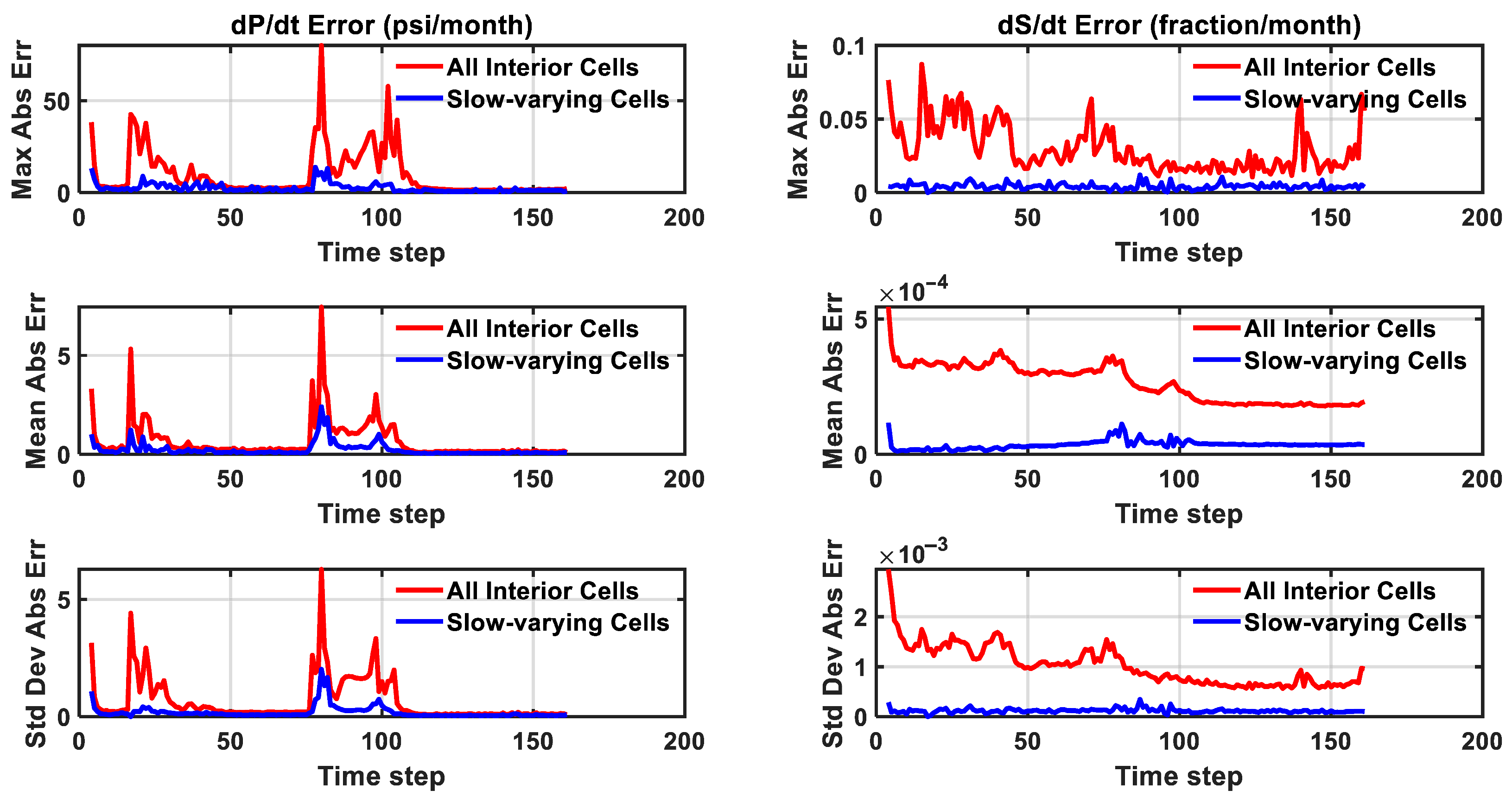
Figure 12 provides a comprehensive analysis of the errors in the models’ predictions for $dP/dt$ and $dS/dt$ over time, comparing two distinct proxy models: one trained using all time instances from the interior cells and another trained exclusively on the slow-varying ones, which constitute 74.4% of the total time instances (968,848 out of 1,302,394). These 1,302,394 instances correspond to the values of 8243 interior grid blocks evaluated over 158 time steps (from time step 4 to 161), for which the ML model generates predictions. The first three time steps are obtained directly from the full-physics simulation and serve as initial conditions, after which the ML model iteratively generates predictions from step 4 onward. Each time step corresponds to one month, as also reflected in Figure 12, where the x-axis shows sequential monthly steps.

The slow-varying cells were identified using the automated ML and IQR-based classifier described in Section 2. As part of this procedure, the hyperparameter $k$ was automatically determined from the respective error distributions of pressure and saturation. This yielded $k=1$ for pressure, where sharper localized transients created narrow error distributions that required a tighter threshold to capture fast-varying cells, and $k=3.5$ for saturation, where a broader error spread necessitated a wider threshold to avoid over-flagging. These data-specific thresholds ensure that classification reflects the distinct statistical behavior of each variable.

Error evaluation was conducted using three metrics: maximum absolute error, mean absolute error, and standard deviation of the absolute error. The results are visualized for the entire set of interior cells (depicted in red) and the subset of slow-varying cells (depicted in blue).

In the case where the model is trained on all interior cells, the maximum error for $dP/dt$ remains relatively low throughout most time steps, with notable spikes occurring between time steps 16–45 and 76–107. These peaks indicate that the model struggles to accurately predict pressure variations during these periods, likely due to intensified reservoir dynamics. The increased error corresponds to abrupt pressure fluctuations driven by well interactions, where injection and production activities induce transient pressure responses. These localized deviations from the overall trend highlight the model’s difficulty in capturing the rapid and complex pressure changes occurring in highly dynamic regions.

This behavior is further reflected in the mean absolute error and standard deviation, both of which increase significantly during these high-variability periods. The elevated standard deviation underscores that these errors are not uniformly distributed across the reservoir but are concentrated in specific regions where pressure changes are abrupt. These zones, typically near wells, experience strong pressure perturbations due to wellbore effects and inter-well interference, making prediction more challenging. However, once these transient effects diminish and the reservoir stabilizes, the error decreases, indicating a return to a more predictable pressure evolution.

In contrast, when the model is trained only on slow-varying cells, the maximum and mean absolute errors remain consistently low, without significant spikes. These cells exhibit smooth and gradual pressure variations, allowing the model to perform reliably under stable conditions. The absence of large fluctuations suggests that the model effectively captures the dominant pressure trends in these regions while avoiding the complexities associated with highly dynamic zones. The lower standard deviation further confirms that the error distribution is more uniform, reinforcing that the primary source of elevated error in the first case is the presence of transient, high-variability regions rather than a general modeling deficiency.

For $dS/dt$, fluctuations in maximum error reflect the complexities introduced by rapid CO₂ plume migration, primarily driven by the reservoir’s high horizontal permeability. As the plume advances laterally, it induces abrupt saturation transitions in previously unsaturated regions, leading to sudden changes in $dS/dt$. These sharp transitions contribute to elevated mean errors in the all-cell model, highlighting the challenge of accurately predicting such dynamic saturation behavior.

This issue is further compounded by reservoir heterogeneities, including preferential flow paths and permeability barriers, which dictate how CO₂ displaces brine. These geological features create spatially uneven and temporally complex saturation patterns, further increasing the difficulty of predicting saturation evolution accurately. Early on, larger errors are observed near the injection zone due to the sudden onset of CO₂ displacement. However, as the plume propagates deeper into the reservoir, significant errors also appear in more distant regions where CO₂ saturation changes remain highly dynamic. As the system stabilizes and saturation transitions slow, the maximum absolute error decreases, indicating improved predictability in later time steps.

On the contrary, when the model is trained only on slow-varying cells, the maximum absolute error remains consistently low across all time steps, with no significant spikes. This suggests that the model performs more reliably when predicting saturation changes in regions where CO₂ migration occurs gradually. By focusing on areas with steady-state behavior, the slow-varying cell model demonstrates greater robustness, effectively avoiding the complexities associated with rapid saturation transitions and improving overall stability in prediction accuracy.

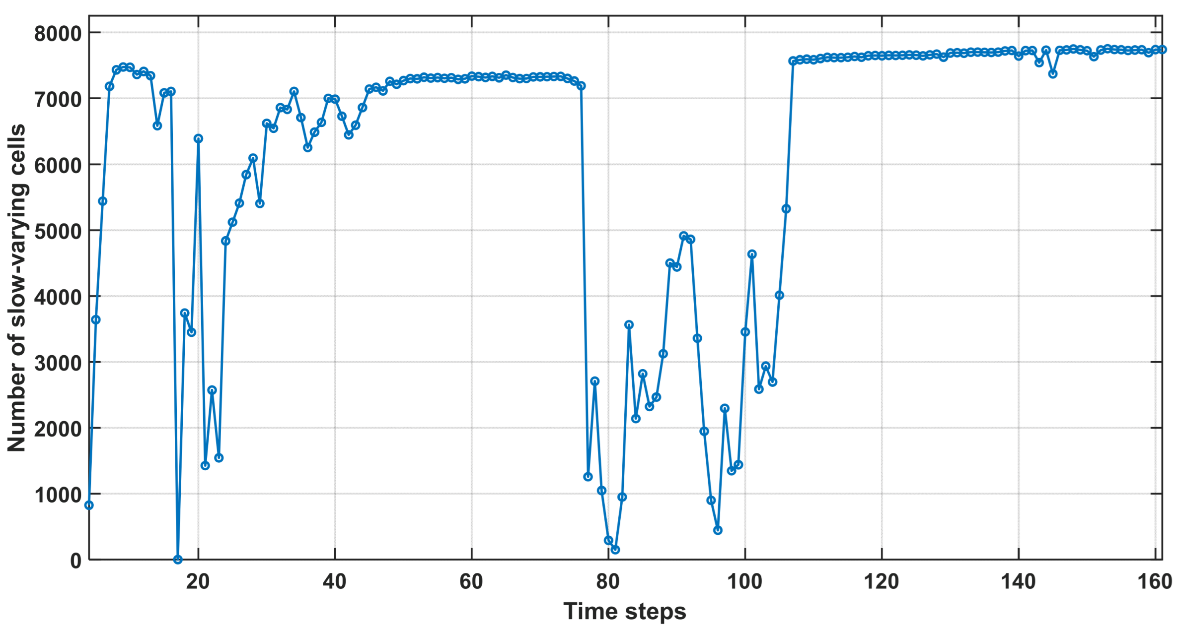
Figure 13 demonstrates the capability of the classification algorithm to effectively capture temporal variations in reservoir dynamics by identifying slow-varying cells throughout the simulation. During periods of heightened instability (time steps 16–45 and 76–107), a pronounced reduction in the number of slow-varying cells is observed, coinciding with rapid fluctuations in pressure and saturation. This decline indicates that a significant portion of the reservoir undergoes abrupt changes, reflecting the dominance of transient flow regimes and localized perturbations. The model’s sensitivity to these dynamic conditions underscores the inherent challenges in accurately predicting saturation and pressure evolution during highly unsteady flow periods.

In contrast, during relatively stable phases (time steps 5–16, 46–76, and 107–161), the number of slow-varying cells increases and asymptotically approaches the total number of interior cells. This trend suggests that the reservoir transitions into a more predictable state, characterized by smoother pressure and saturation gradients. The stabilization of the slow-varying cell count during these periods indicates a shift towards quasi-equilibrium conditions in most regions of the reservoir, where transient effects have diminished, and CO₂ plume migration is mostly capillarity and gravity driven.

To further investigate the factors driving these periods of sudden changes, Figure 14, Figure 15 and Figure 16 present the operational performance of the three CO₂ injection wells (I1, I2, and I3) and eight production wells (P1 to P8) throughout the injection process within the brine-filled reservoir. 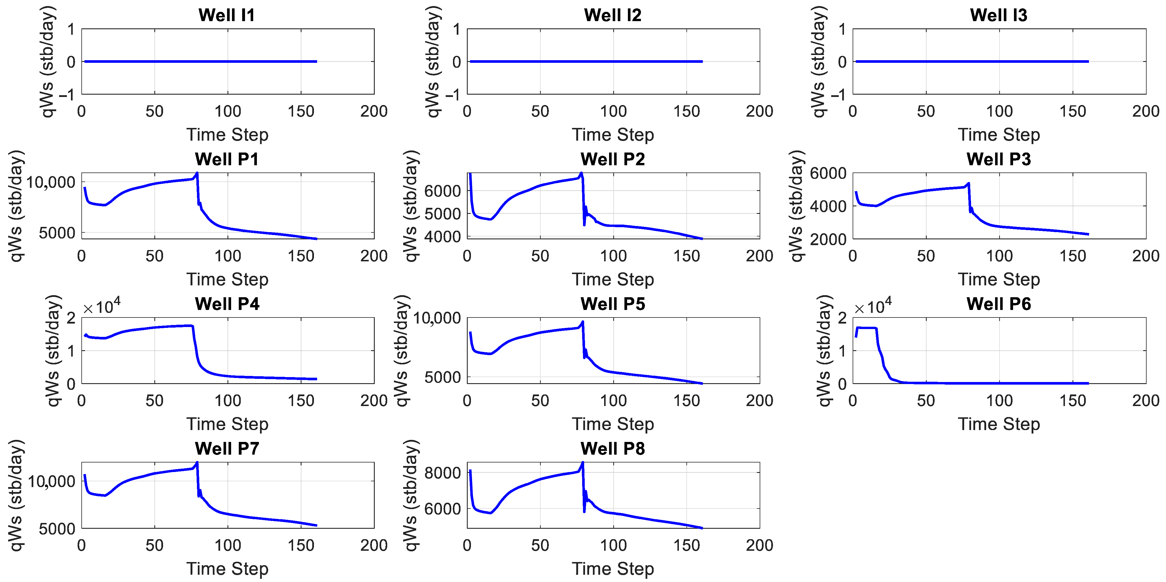Figure 14 illustrates the gas flow rate (qGs) for each well in standard cubic feet per day (scf/day), Figure 15 depicts the brine flow rate (qWs) in stock tank barrels per day (stb/day), and Figure 16 displays the bottom-hole pressure (BHP) in pounds per square inch (psi). The injectors (I1, I2, and I3) are grouped in the top row, while the producers (P1 to P8) are shown in the subsequent rows. These figures provide a comprehensive visualization of the temporal evolution of well operational parameters, offering key insights into how CO₂ injection dynamics influence fluid displacement and pressure distribution within the reservoir. By analyzing these trends, it becomes possible to correlate well activity with abrupt changes in pressure and saturation.

In the injector wells (I1, I2, I3), qWs remains at zero throughout the simulation, confirming that no brine injection or production occurs in these wells. However, the gas injection behavior varies across the injectors, reflecting heterogeneities in reservoir properties and connectivity. A key observation is that in all injectors, a noticeable BHP buildup begins at timestep 17, followed by a sharp increase in BHP from timestep 17 to 45. This period marks a critical phase in the injection process, as the reservoir undergoes pressure adjustments in response to CO₂ displacement and evolving fluid distribution.

Well I1 initially exhibits a high and stable qGs, indicating strong injectivity, likely due to favorable near-wellbore conditions such as high permeability. However, as injection progresses, qGs experiences a sharp decline after time step 96, signaling substantial pressure buildup that reduces the pressure differential driving injection. This trend is further corroborated by the BHP, which steadily increases and plateaus at the imposed 9000 psi limit by time step 97. The steep decline in injectivity between time steps 96 and 107 introduces instability in the region, as evidenced by the fluctuations observed in Figure 14.

In contrast, Well I2, situated near producer P6 (see Figure 9) within the forked aquifer region, exhibits a more gradual increase in qGs during the early stages of the simulation. At timestep 97, qGs spikes sharply as the BHP reaches its upper constraint, followed by a steady decline until time step 107. This behavior indicates a slower pressure buildup in the vicinity of I2 compared to I1, primarily due to its proximity to P6. The localized pressure sink created by P6 enhances injectivity by facilitating CO₂ and brine migration toward the producer, thereby mitigating immediate pressure accumulation around I2. Additionally, the delayed pressure buildup near I2, relative to I1 and I3, underscores the influence of well placement and reservoir connectivity on injection dynamics.

Well I3 initially exhibits a high qGs, similar to I1; however, its decline is more gradual, indicating sustained but progressively decreasing injectivity as CO₂ saturation increases around the well. Notably, qGs, for I3 begins to decline earlier than in I1, even before reaching the BHP constraint at time step 97. This early decline is attributed to faster pressure buildup in a less connected reservoir region. The steady rise in BHP for I3 further corroborates this localized pressure response. Additionally, both I2 and I3 exhibit lower initial injection rates compared to I1, highlighting the superior permeability and injectivity in the area surrounding I1.

Regarding the production wells, all producers except P6 exhibit similar trends in BHP and production rates during the early simulation phase. For most producers, BHP remains stable at the imposed lower limit of 3000 psi until time step 79, at which point it begins to increase steadily. This initial stability suggests that the pressure sinks generated by the producers are effectively counterbalanced by the reservoir’s natural pressure support, as well as the pressure increase resulting from CO₂ injection. However, beyond time step 79, the gradual rise in BHP indicates localized reservoir pressure depletion as production continues, reducing the pressure differential driving fluid withdrawal.

A notable pattern among the producers, excluding P6, is the sharp increase in qWs between timesteps 17 and 45. This early surge in brine production likely reflects high brine mobility and the rapid drainage of brine near these wells during the initial production phase. In contrast, P6 exhibits a decrease in qWs after timestep 17, likely due to its proximity to the injectors. The closer location to injection wells facilitates faster pressure redistribution, delaying the sharp brine influx and altering brine production dynamics near P6.

The qGs trends, as shown in Figure 14, vary across the producers, reflecting differences in reservoir connectivity and the timing of CO₂ breakthrough. Producer P6 exhibits a distinct behavior, initiating CO₂ production at timestep 17, with flow rates stabilizing rapidly by time step 20. This early and sustained CO₂ breakthrough is attributed to P6’s close proximity to the injectors, which facilitates rapid gas migration.

Similarly, P4 experiences CO₂ breakthrough later in the simulation, beginning at time step 76 and stabilizing almost immediately by time step 79. This delayed response suggests a slower CO₂ migration pathway, likely due to P4’s greater distance from the injection wells, resulting in prolonged brine displacement before gas reaches the wellbore. For the remaining producers, qGs generally exhibits a steady increase over time, reflecting progressive CO₂ breakthrough at these wells.

Realistic reservoir systems are inherently complex, and this complexity escalates with an increasing number of wells due to the intricate interplay of pressure and saturation dynamics. Fast-varying regions are not confined to areas immediately surrounding wells; over time, pressure diffusivity causes these dynamics to propagate outward, affecting grid blocks farther from the wells. This propagation further complicates the task of identifying fast-varying regions, making manual classification impractical.

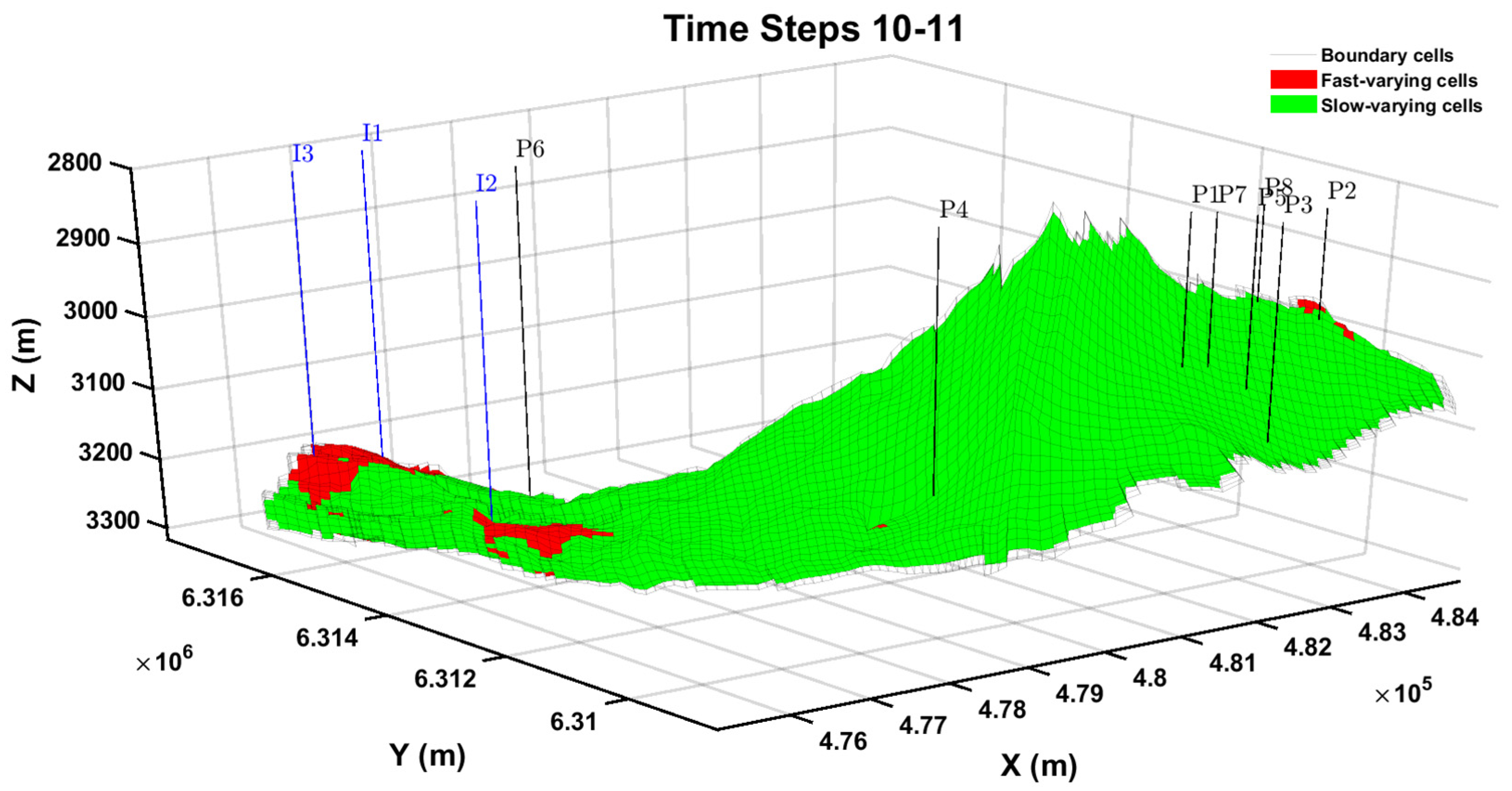
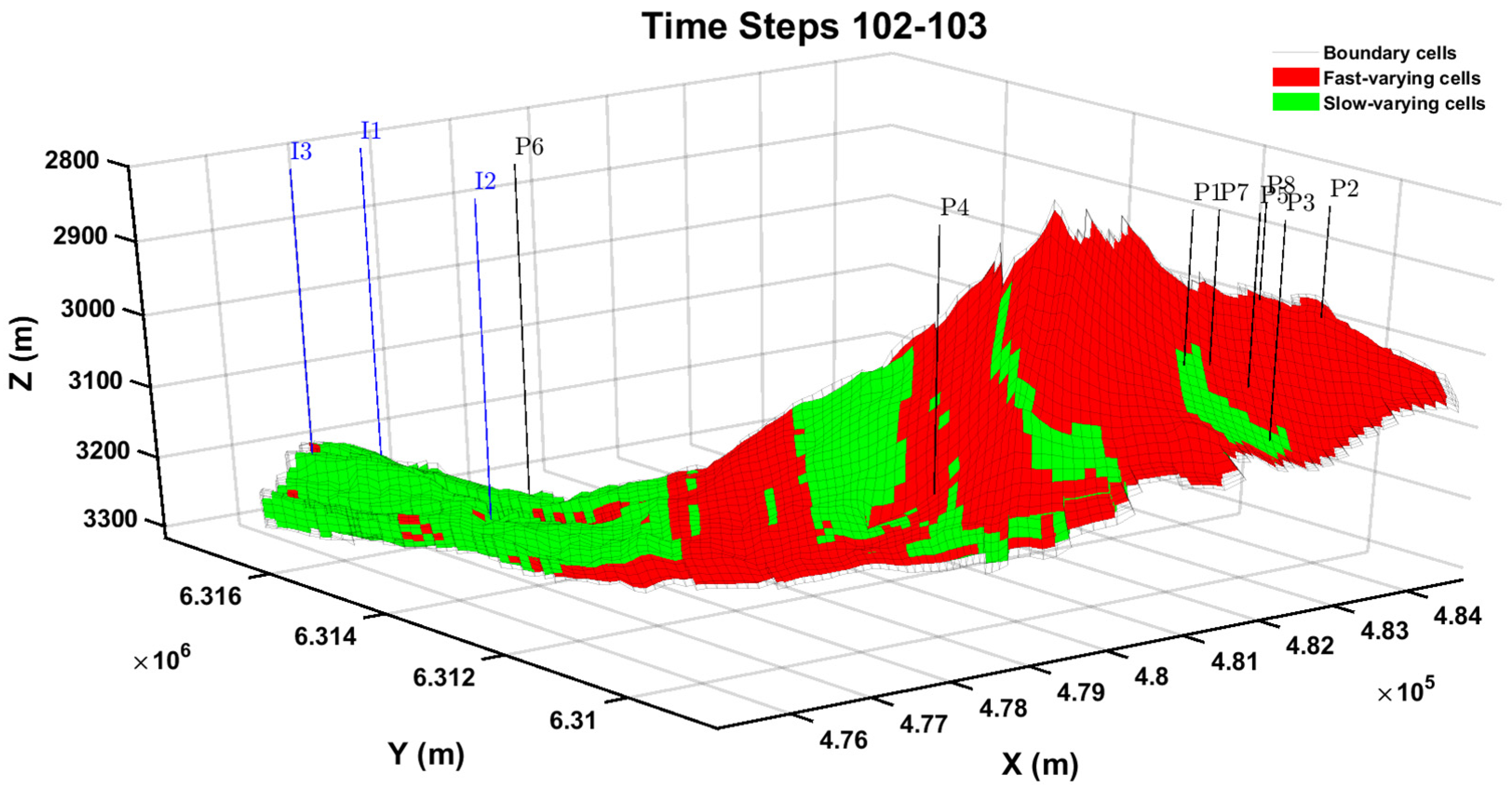
To provide further insight into how the classification algorithm identifies dynamic reservoir regions, a series of figures was prepared at selected time intervals. These figures illustrate the spatial distribution of classified grid blocks, where green cells represent slow-varying regions, red cells indicate fast-varying regions, and white cells denote boundary areas excluded from the analysis. By examining these visual representations, a clearer understanding of the temporal and spatial evolution of slow- and fast-varying regions can be obtained, offering valuable insights into how reservoir dynamics evolve over time.

Specifically, Figure 17, which depicts the classified grid blocks during the transition between time steps 10 and 11, provides a detailed snapshot of the reservoir’s dynamic behavior in the early stages of the simulation. This time interval was specifically selected as pressure diffusivity remains limited, resulting in pressure changes that are predominantly localized around the wells. The classification highlights fast-varying regions concentrated near the injection wells, where CO₂ injection induces significant pressure and saturation variations due to rapid fluid displacement and the formation of gas-saturated zones. Conversely, slow-varying regions dominate the reservoir grid, particularly in areas farther from the wells, where pressure and saturation remain largely undisturbed at this stage. This classification framework effectively captures the early evolution of reservoir dynamics, emphasizing the strong localized effects of injection while illustrating the gradual expansion of pressure and saturation perturbations as the simulation progresses.

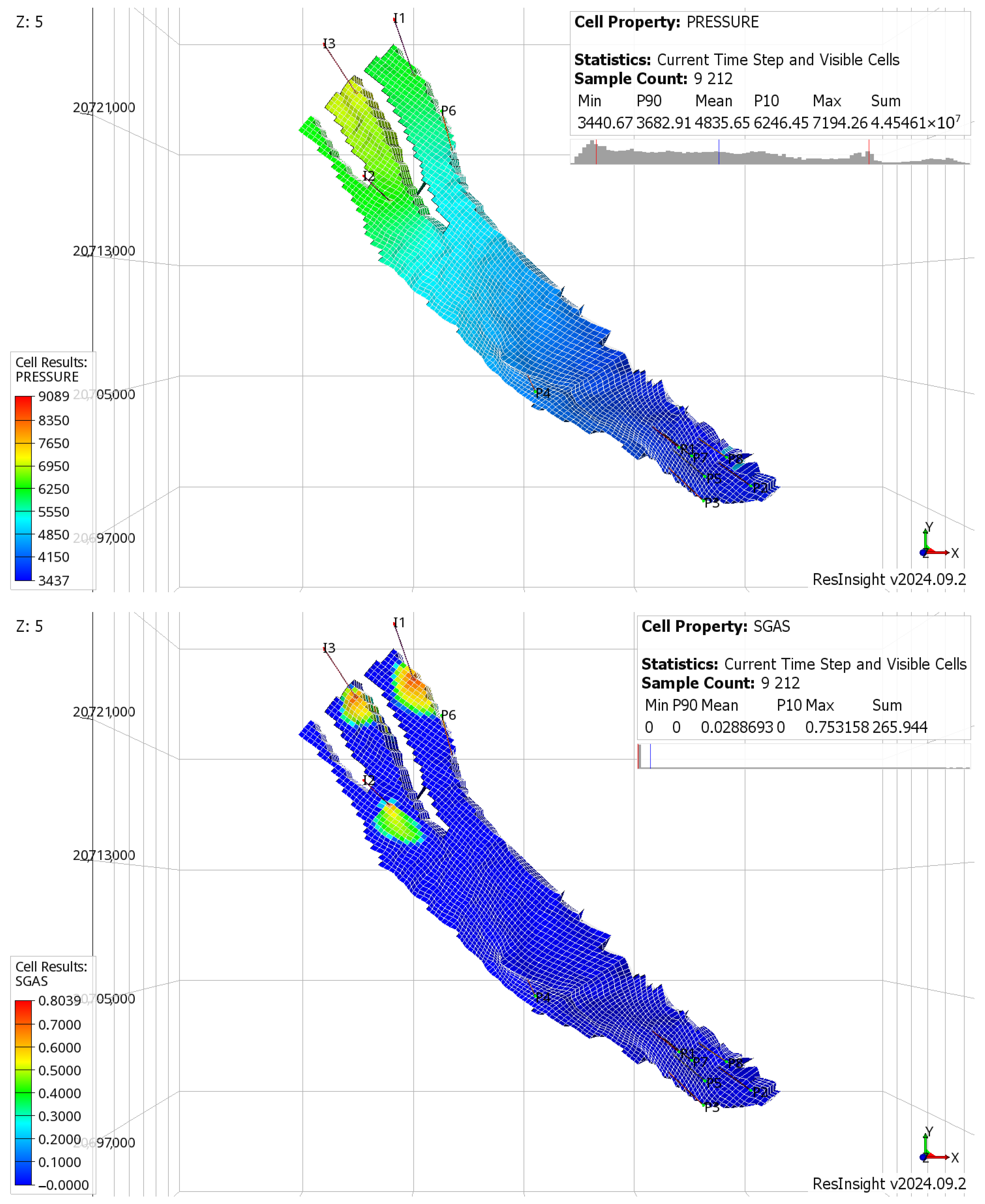
The accompanying pressure distribution plot (Figure 18) further corroborates the classification results for time steps 10 to 11, illustrating elevated pressures in the regions surrounding the injectors. Notably, the highest pressure buildup is observed near I3, reflecting its inferior injectivity and the resulting localized pressurization effects. The areas surrounding the production wells, including P6, also exhibit pressure responses, though these are less pronounced compared to the injection zones. These patterns highlight the localized influence of CO₂ injection and brine displacement, with pressure gradients gradually diffusing outward over time as reservoir equilibrium evolves.

Additionally, the CO₂ saturation distribution plot (Figure 18) reveals that the areas immediately surrounding the injection wells are already saturated with CO₂, confirming that gas flooding has begun in these regions. This early CO₂ saturation near the injectors further validates the classification framework, which identifies fast-varying regions where pressure and saturation changes are both abrupt and dynamic. These observations reinforce the effectiveness of the classification in distinguishing transient flow behavior and provide critical insight into the early-stage migration of CO₂ within the reservoir.

Figure 19, depicting the classified grid blocks for the transition between time steps 75 and 76, reveals a reservoir predominantly characterized by slow-varying cells. This classification reflects the absence of abrupt operational changes in both the injection and production wells during this period. The injectors maintain steady injection rates, while the producers exhibit consistent production behavior, resulting in a stable reservoir state with minimal dynamic variations.

However, a closer examination highlights the presence of fast-varying cells concentrated in specific regions, particularly where the CO₂ plume has recently arrived, as evidenced in the CO₂ saturation distribution plot (Figure 20). These localized regions of fast variation are directly linked to the ongoing migration of the CO₂ plume, where changes in gas saturation induce transient flow behavior.

The predominance of slow-varying cells across the reservoir grid underscores the overall stability of the system at this stage of the simulation, with only localized areas exhibiting transient dynamics. This classification aligns with the reservoir’s gradual transition toward a quasi-steady state, as injected CO₂ continues to spread and displace brine. These observations reinforce the classifier’s ability to capture subtle yet critical variations in reservoir behavior, providing valuable insights into the evolving flow dynamics and spatial distribution of CO₂ within the system.

During time steps 102–103, the classification results indicate that the majority of grid cells near the injection wells are identified as slow-varying (Figure 21). This behavior can be attributed to the constant bottom-hole pressure (BHP) of 9000 psi maintained for all injectors, signifying a lack of significant operational changes in this region. As a result, reservoir conditions near the injectors remain stable, with fluid flow dynamics exhibiting gradual and predictable variations. In contrast, reservoir behavior near the production wells, particularly on the opposite side of the structural high, exhibits a markedly different trend. As shown in Figure 16, the BHP of the producers is undergoing a rapid increase, leading to dynamic changes in the local pressure field. Simultaneously, qWs is decreasing sharply (Figure 15), further contributing to abrupt transitions in reservoir properties. These operational adjustments in the production sector induce fast-varying behavior, as reflected by sharp changes in pressure gradients and fluid flow dynamics. The classification framework effectively captures these shifts, highlighting the strong correlation between production-induced pressure variations and transient reservoir behavior. These findings emphasize the importance of monitoring production constraints and pressure redistribution to better understand the evolving flow dynamics within the system.

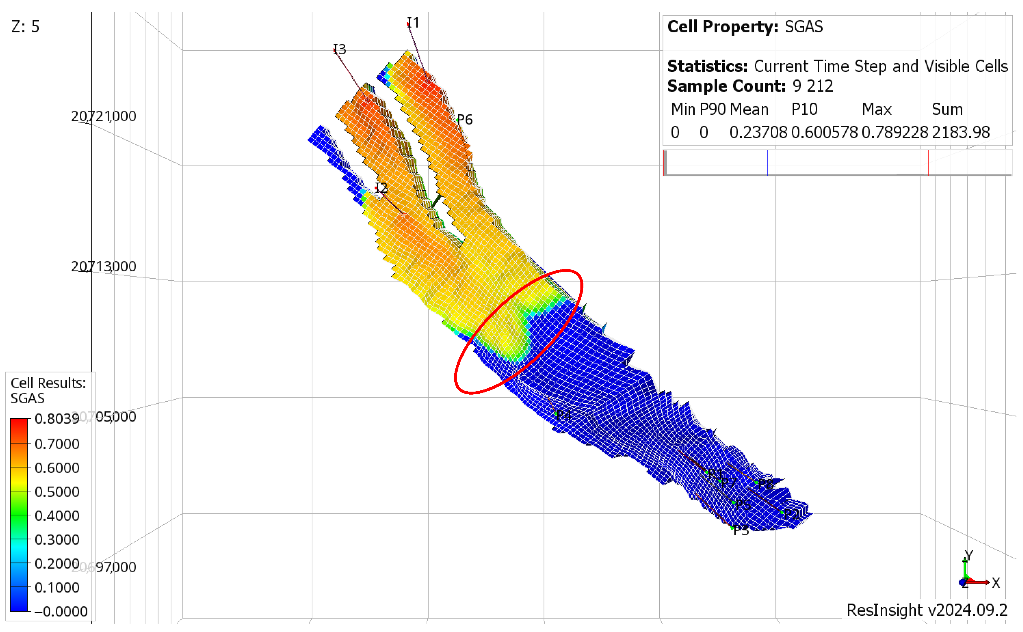
During this period, P4 does not undergo significant operational changes; however, the region classified as fast-varying around P4 aligns with the arrival of the CO₂ plume, as observed in Figure 22. The introduction of the plume results in sharp saturation changes and localized pressure variations, causing these grid cells to exhibit dynamic behavior despite the well’s stable operational parameters. This observation underscores the influence of reservoir heterogeneities and fluid front dynamics in generating localized fast-varying regions, independent of direct changes in well operation.

Furthermore, Figure 21 highlights distinct fast-varying zones surrounding P4, providing additional insights into pressure propagation mechanisms. The red area preceding P4 represents regions where pressure diffusivity from prior abrupt events near the injectors has propagated, illustrating the delayed transmission of pressure disturbances from earlier injection activity. Conversely, the red area beyond P4 corresponds to zones influenced by pressure diffusivity associated with both the injection and production wells from previous time steps. This spatial distribution demonstrates the overlapping effects of pressure propagation from multiple sources, creating a complex interplay of dynamic reservoir behavior that manifests as fast-varying regions. These findings emphasize the necessity of considering both direct and indirect reservoir responses when analyzing transient flow behavior and predictive modeling in heterogeneous systems.

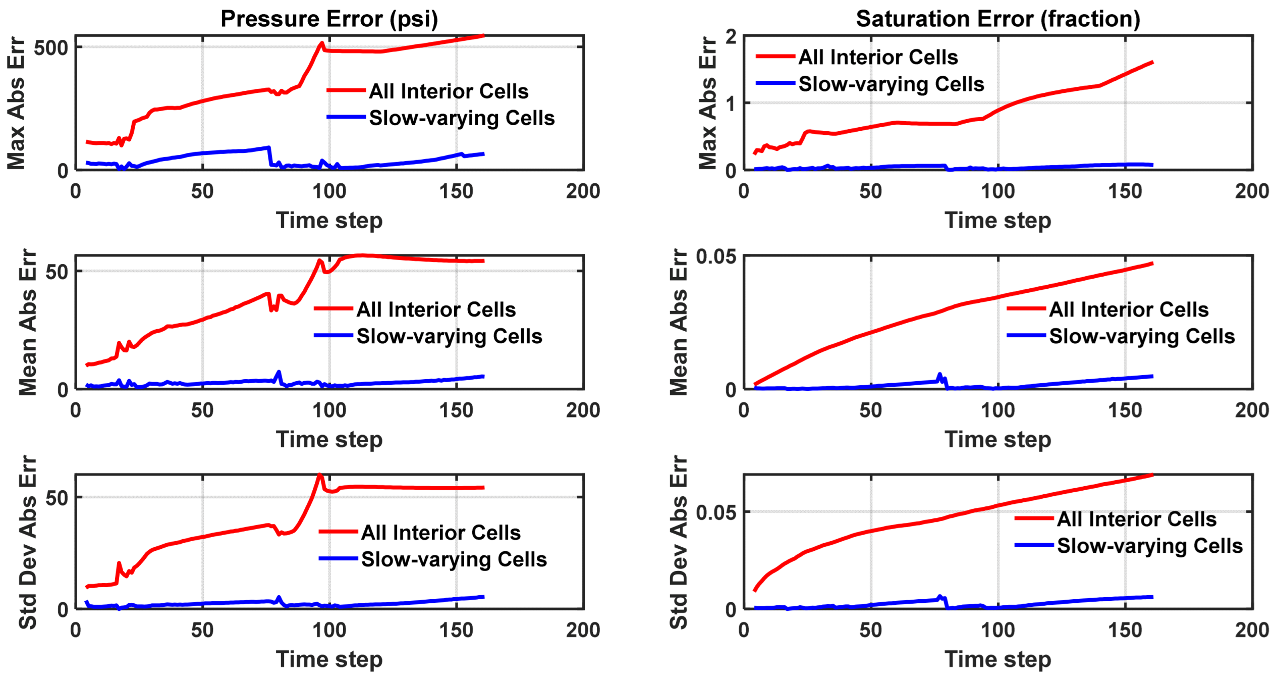
Figure 23 provides a comprehensive comparison of the errors in pressure and saturation predictions over the entire 40-year simulation period, illustrating how these errors accumulate under different modeling approaches. In the first case, where all grid blocks are considered and the proxy model operates independently of the nonlinear solver, errors in both pressure and saturation exhibit a steady increase over time. The maximum, mean, and standard deviation of these errors progressively rise, indicating a compounding effect as deviations from the reference solution grow. Over extended time scales, this accumulation becomes significant, ultimately rendering the proxy model’s predictions unreliable. This trend underscores the challenges associated with long-term predictive modeling in complex reservoir systems, particularly when simplified approximations are used without continuous correction from high-fidelity numerical solvers.

At the midpoint of the simulation (20 years), the mean error in pressure for the case in which all interior cells are considered reaches approximately 40 psi, while the mean saturation error rises to 0.03 in fraction. In contrast, when only slow-varying cells are considered, the mean pressure error remains significantly lower at approximately 2 psi, and the mean saturation error is reduced to 0.0004 in fraction. This substantial discrepancy highlights the enhanced predictive accuracy achieved by selectively focusing on slow-varying cells, effectively reducing numerical error propagation and improving model stability.

By the end of the 40-year simulation, error accumulation becomes even more pronounced. When all interior cells are included, the pressure error escalates to approximately 54 psi, while the saturation error increases to 0.047 in fraction. Conversely, in the slow-varying cell approach, the pressure error remains significantly lower at approximately 5 psi, with the saturation error constrained to just 0.005 in fraction. These findings underscore the efficacy of the proposed methodology in mitigating long-term error accumulation, thereby enhancing the robustness of reservoir simulations. By prioritizing slow-varying regions, this approach offers a more reliable framework for long-term reservoir modeling, ensuring greater accuracy in predictive simulations while reducing computational inefficiencies.

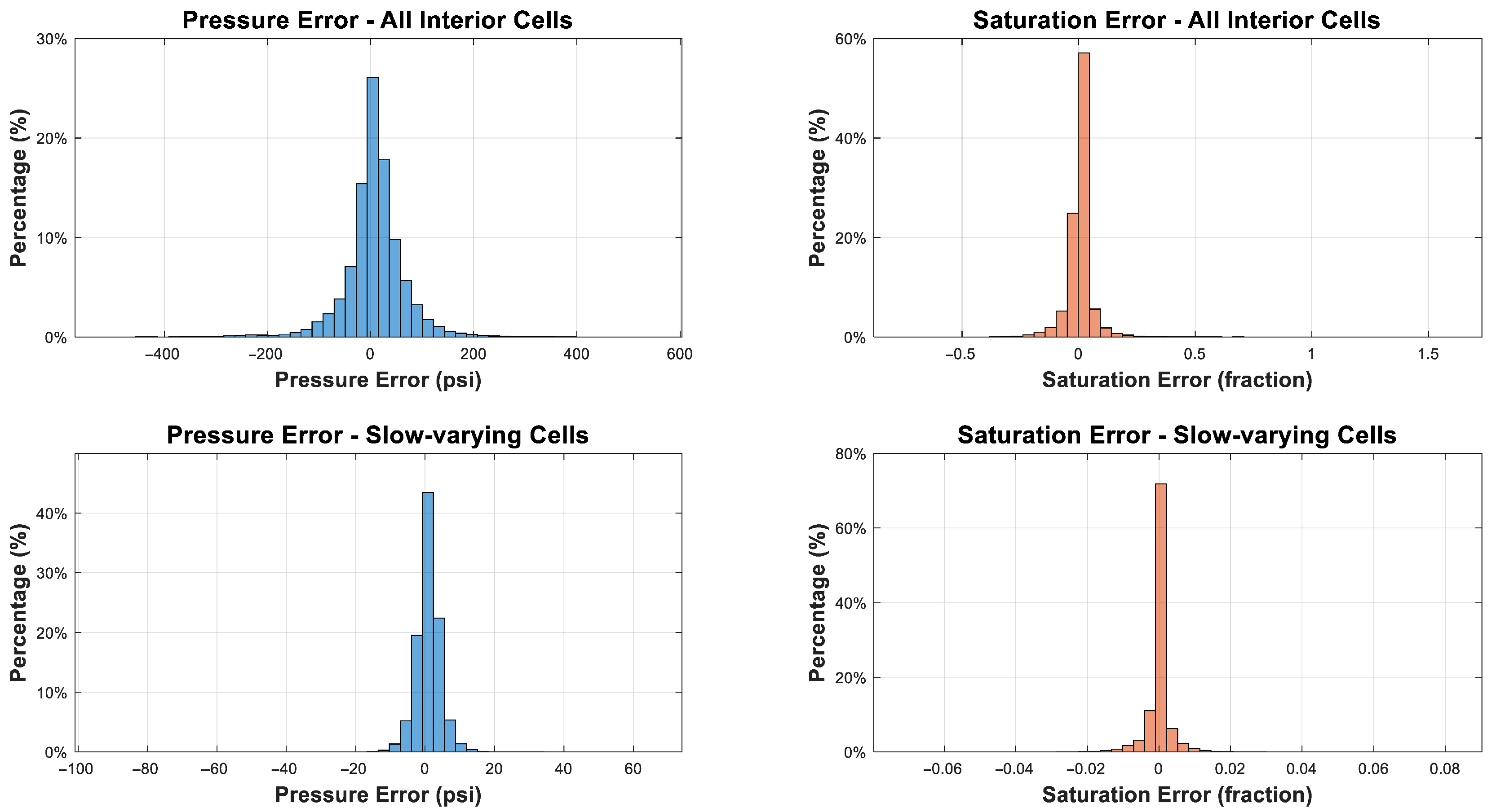
Building on the analysis presented in Figure 23, the histograms in Figure 24 offer a more detailed examination of the error distributions in pressure and saturation predictions for the two modeling approaches: one incorporating all interior cells and the other focusing exclusively on slow-varying cells. These distributions provide a complementary perspective on the propagation of errors across the reservoir and time domain, further illustrating the disparities in predictive accuracy between the two ML models. By quantifying the frequency and magnitude of errors, these histograms highlight the effectiveness of the slow-varying cell approach in reducing overall error accumulation and improving the reliability of long-term reservoir simulations.

For the case where all interior cells are included, the histogram of pressure errors reveals a broader distribution centered near zero but with substantial variability. Errors predominantly range between −200 and 200 psi, with outliers extending beyond ±400 psi, underscoring significant inaccuracies in some regions. The saturation errors in this case similarly display a pronounced peak around zero, but with a skewed tail reaching as high as 1.5 in fractional error. These large deviations indicate localized challenges in capturing the complex dynamics of saturation across the full domain.

Conversely, when focusing on slow-varying cells, the error distributions are notably tighter and more symmetric around zero. The pressure errors are concentrated within the range of −20 to 20 psi, reflecting a much higher degree of accuracy in these smoother regions. Similarly, the saturation error distribution is sharply peaked, with most values constrained between −0.06 and 0.08 in fractional error. This indicates that the methodology significantly reduces variability and achieves consistently reliable predictions in areas with gradual spatial changes.

These results reinforce the trends observed in Figure 23, where the cumulative error metrics highlighted the stark differences between the two cases. The histograms further illustrate that by prioritizing regions with slow spatial variations, the proposed methodology not only minimizes error accumulation over time but also ensures greater spatial consistency in predictions. This combination of reduced long-term error growth and localized accuracy demonstrates the robustness and practicality of the slow-varying cells approach for long-term reservoir simulation and prediction tasks.

This error accumulation can be better understood by examining how pressure and saturation predictions evolve at each time step. Each predicted state at time step $t_{i+1}$, denoted as ${\widehat{P}}_{i+1}$ and ${\widehat{S}}_{i+1}$ is computed using the formulas:

$${\widehat{P}}_{i+1}={\widehat{P}}_i+{\widehat{{\displaystyle \frac{dP}{dt}}}}_i\left(t_{i+1}-t_i\right)$$

(4)

$${\widehat{S}}_{i+1}={\widehat{S}}_i+{\widehat{{\displaystyle \frac{dS}{dt}}}}_i\left(t_{i+1}-t_i\right)$$

(5)

While the error at a single time step may appear negligible, it propagates and compounds over successive time steps, leading to a cumulative effect. Over an extended sequence of time steps, this accumulation becomes increasingly significant, ultimately resulting in substantial deviations from the true system state. The absence of feedback from the nonlinear solver further exacerbates this issue, as there is no corrective mechanism to realign the model’s predictions with the actual reservoir dynamics. Consequently, the compounded errors can progressively degrade model accuracy, particularly in long-term simulations, underscoring the critical need for error mitigation strategies in data-driven reservoir modeling.

In contrast, the second approach employs a hybrid methodology in which regions of the grid experiencing rapid changes in pressure and saturation are selectively excluded from ML-based predictions. Instead, the nonlinear solver is applied in these dynamically evolving regions to provide more accurate estimates of $P_i$ and $S_i$ at critical time steps, thereby mitigating error accumulation in areas most susceptible to transient behavior. For grid blocks where pressure and saturation variations remain gradual, the ML model continues to make predictions, as the risk of significant error accumulation is considerably lower in these zones.

As illustrated in Figure 23 and Figure 24, this hybrid approach yields substantially more stable and accurate results over time, with errors remaining consistently lower compared to the fully ML-driven case. The strategic exclusion of fast-varying regions from ML-based predictions proves highly effective in preserving model fidelity, underscoring the advantages of adaptive modeling in reducing long-term error propagation. This methodology highlights the importance of integrating physics-based corrections into data-driven models to enhance predictive reliability in complex reservoir simulations.

5. Conclusions

This study applied an automated machine learning (ML)-driven grid block classification framework to a real world deep saline aquifer model, demonstrating its potential for accelerating numerical simulations of CO₂ geological storage. By integrating machine learning techniques with an interquartile range (IQR)-based classifier, the methodology effectively identified fast- and slow-varying grid blocks, optimizing computational efficiency while maintaining predictive accuracy. The results confirmed that restricting the ML-based proxy model to slow-varying grid blocks significantly reduced computational costs without compromising the reliability of the simulations.

This work serves as a validation of the proposed hybrid methodology, limited to a single scheduling scenario designed to explore its capabilities. Future research should focus on expanding the dataset to include a broader range of subsurface conditions, capturing diverse injection and production scenarios as well as variations in petrophysical properties such as permeability and porosity distributions. Importantly, these datasets must be generated with a high degree of generality to ensure robustness and adaptability across different geological settings.

Moreover, strict adherence to subsurface regulatory frameworks and industry best practices for CO₂ storage and reservoir simulation is essential for real-world applicability. Compliance with these standards ensures that the methodology remains relevant for field-scale projects, where operational safety, regulatory approval, and long-term containment integrity are critical considerations. By aligning simulation outputs with established guidelines, this approach can support informed decision-making and facilitate formal reporting processes in CO₂ storage initiatives.

Overall, this study highlights the potential of ML-driven methodologies to enhance computational efficiency in reservoir simulations while maintaining predictive accuracy. By addressing the identified limitations and ensuring regulatory compliance, future advancements in this approach could contribute significantly to optimizing large-scale CO₂ sequestration strategies.