An Extended Model Approach to Study the Power Flow Analysis of Complex Power Systems

Abstract

This paper focuses on the reconfigurability of power system extension models and improves the adaptability of radiation distribution network schemes to complex power networks. The existing Newton–Raphson based solutions face difficulties in reconstructing dynamics, often failing to converge or requiring high initial condition settings in extended systems. For the IEEE 30-bus system, based on node-provided data, we optimized the Newton–Raphson algorithm model for practical complex power systems. The novel optimization algorithm leverages multi-radiation power grid reconfiguration, significantly reducing dependencies on optimization time and initial state reconstruction. The results verify the effectiveness of the model and algorithm.

1. Introduction

With the continuous expansion and extension of the power grid system, the analysis and calculation methods of the power grid system is more significant. The continuous extension of the power grid system has different characteristics. The reconstruction of the distribution network is meant to reduce network loss, balance load, eliminate overload, improve voltage distribution, enhance power supply quality, and improve system economy and power supply reliability by changing the opening and closing states of the interconnection switches and section switches in the line, in order to satisfy system constraints. Power system reconstruction refers to isolating faults and recovering power by changing the topology structure of the power grid [1,2]. The paper’s power system reconstruction is aimed at analyzing and comparing the system performance of a new complex system after topology extension on the original system.

The comprehensive power system of ships exhibits complex mixed dynamics during reconstruction, and some equipment in the system is designed to reduce the problem of excessive discrete states caused by the expansion of the system scale. When the ship’s integrated power system fails, reconstruction is a technology that ensures continuous power supply and load balancing by changing the power grid topology and isolating the fault area [3,4], transferring high-quality power to important loads to minimize the threat caused by disturbances or faults [5]. Belkacemi et al. improved system reliability through distribution network reconstruction, but the response time of centralized control is slow. This is not conducive to real-time scheduling, is highly dependent on the central controller, and is prone to single point failures, resulting in relatively poor reliability [6,7]. Distributed control can overcome the above disadvantages in traditional centralized control and has the advantages of less information transmission and high reliability in achieving real-time control of the internal autonomy of the active distribution network [8]. Research on ship power system reconstruction mostly deals with single-point random failure problems by improving the ability to optimize the algorithm under a centralized control structure [9,10,11].

Multi-agent systems are combined with immune algorithms to carry out fault detection, isolation, and power grid reconstruction operations. Wang et al. [10] applied a multi-agent ant colony algorithm to the network reconstruction of a ship integrated power system, and showed that the addition of a multi-agent system to the ant colony algorithm accelerated the convergence speed of the algorithm and improved real-time performance. A multi-agent particle swarm optimization algorithm for a ship integrated power system has been proposed, which improves the optimization ability and speed of the algorithm [11]. A three-layer hierarchical control strategy was designed, which adds a centralized reconstruction layer on the basis of the distributed control layer and combines with the genetic algorithm for optimization calculation [12].

On this basis, probabilistic power flow (PPF) models are commonly constructed using Monte Carlo simulation (MCS) [13,14]. Related research results have been achieved, and the analysis of the characteristics of the structure of the power system after changes has been carried out [15]. Reference [16] proposes a method to eliminate excessive branch power flow in the power system by introducing sensitivity and distribution factors to improve the particle swarm optimization (PSO) algorithm. The proposed algorithm integrates Newton’s iterative process with Wirtinger calculus, enabling linearization of power flow equations directly in the complex plane in reference [17]. These methods improve and enhance power flow analysis in modern distribution systems.

Reconstruction is an important feature for adapting to the integration of new energy into the power grid, and also provides an important reference for the analysis of power system reconstruction. However, in scenarios where the continuous expansion of the power grid faces complex reconfiguration, traditional N-R power flow calculation methods often encounter convergence difficulties and high sensitivity to initial conditions due to the increased system scale, dynamic structural changes, and hybrid characteristics, which severely restrict the analysis efficiency of reconfiguration schemes. To overcome the limitations of the traditional N-R method in expanding complex systems, this study proposes an optimization algorithm based on multi-radial grid reconfiguration technology. The core of this algorithm lies in decomposing complex networks into radial subnets to find rapid solutions, and to achieve global convergence through coordination of tie lines. This method aims to significantly reduce dependence on optimization time and initial state settings, and to enhance the adaptability and computational efficiency of power flow calculation in the analysis of extended system reconfiguration. It has been validated on multiple complex networks including IEEE 30-bus, 57-bus, 118-bus, 162-bus, and 300-bus extended systems.

2. Analyze and Optimize Algorithms

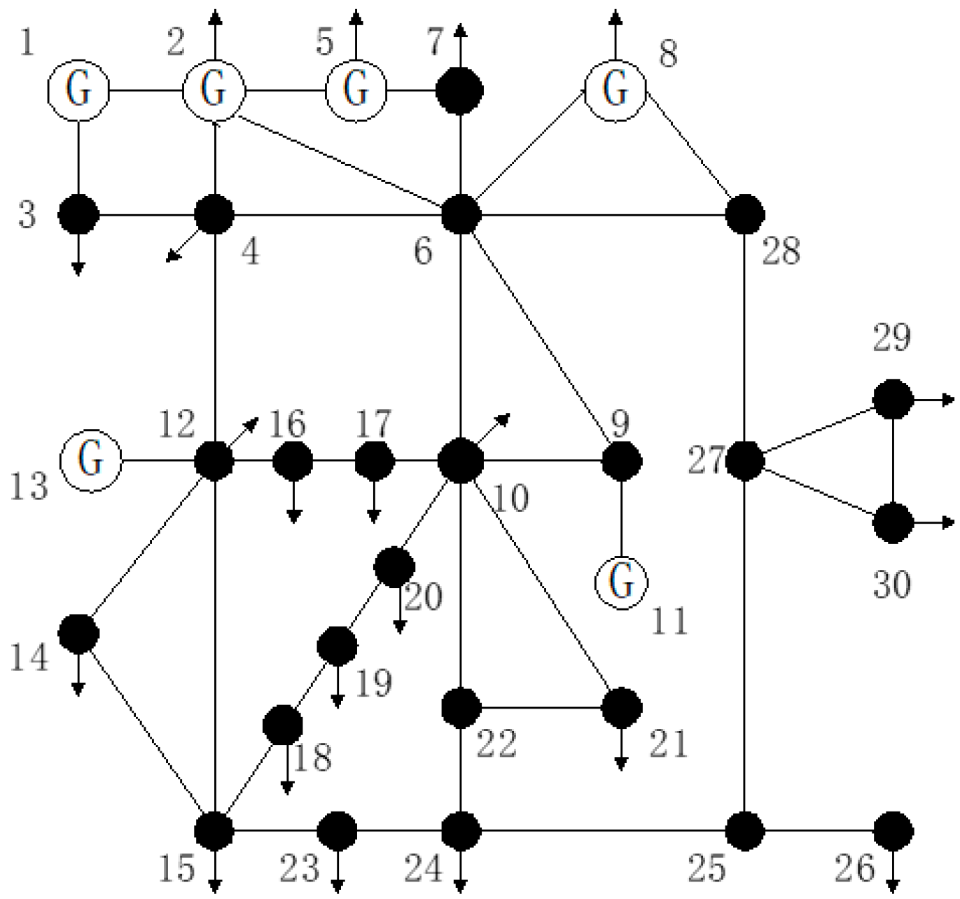
The paper focuses on the power flow analysis and calculation of complex power systems, and iteratively calculates nonlinear equations based on simulation examples of IEEE 30 bus system. Power flow analysis and calculations are performed on various design schemes of the system network to obtain the parameters of each node in different types of power systems, thereby obtaining power flow distribution data of the power system. The Newton–Raphson method can be used to solve nonlinear equations and provide the parameters for system operation [7].

The expansion of the model has resulted in differences in the performance of the system model. Therefore, expanding the existing model topology by adding components such as transmission and distribution should be taken into consideration in order to achieve a regular topology structure, which can reveal the relevant characteristics of the model expansion.

The IEEE 30 bus system wiring diagram is shown in Figure 1.

The flow of distributed power sources connected to the distribution network changes and expands the nodes. The original topology remains unchanged, and the new topology is compared based on the original changes. After the expansion, the system performance changes, and the original system node topology performance tends to converge with the system topology node performance after the expansion.

2.1. Extended System Constraints

The reconstructed distribution network meets the requirements of no “circuits” and no “islands”. In addition to network structure constraints, considering the multi-state switching characteristics of power loads in energy storage systems, the following constraints must be met:

(1)

Equality constraint

$$\begin{array}{c}f(M_{P1},M_{P2},\dots M_{Pn};M_{Q1},M_{Q2},\dots M_{Qn};C_{PQ1},C_{PQ2},\dots C_{PQn};\\ \hspace{1em}\hspace{1em}\hspace{1em}\hspace{1em}\hspace{1em}\hspace{1em}{L}_{PL1},L_{PL2},\dots L_{PLi}; L_{QL1},L_{QL2}\dots L_{QLi})=0\end{array}$$

(1)

In Equation (1), $M_{G\mathrm{i}}$ and $M_{\mathrm{Qi}}$ are the active and reactive power output vectors of different energy sources in the system, respectively; $C_{PQi}$ is the energy storage state. When it is a power source, the attribute is the same as $M_{\mathrm{Pi}}$/$M_{Qi}$. When it is a load, the attribute is the same as $L_{PLi}$/$L_{QLi}$. $L_{PL}$ and $L_{QL}$ are the active and reactive power demand vectors of the load, respectively $i=1,2,\dots n$.

(2)

Inequality constraint

$$\begin{array}{l}g(M_{P1},M_{P2},\dots M_{Pn};M_{Q1},M_{Q2},\dots M_{Qn};C_{PQ1},C_{PQ2},\dots C_{PQn};\\ \hspace{1em}\hspace{1em}\hspace{1em}\hspace{1em}\hspace{1em}\hspace{1em}\hspace{1em}\hspace{1em}\hspace{1em}\hspace{1em}\hspace{1em}{V}_1,V_2,\dots V_i; S_1,S_2\dots S_i)\le 0\end{array}$$

(2)

In Equation (2), $V_{\mathrm{i}}$ is the node voltage vector; $S_i$ is the branch power vector.

2.2. The Power Flow Equation of the System

The following is the basic format of the power flow equation, which is the solution of power imbalance [17]:

$$\left\{\begin{array}{l}\Delta P_i=P_{Gi}-P_{di}-U_i{\displaystyle \sum _{j=1}^n{U}_j}(G_{ij}\cos {\delta }_{ij}+B_{ij}\sin {\delta }_{ij}),i=1,2,\dots n\\ \Delta Q_i=Q_{Gi}-Q_{di}-U_i{\displaystyle \sum _{j=1}^n{U}_j}(G_{ij}\sin {\delta }_{ij}-B_{ij}\cos {\delta }_{ij}),i=1,2,\dots n\end{array}\right.$$

(3)

As shown in the above equation, there are a total of two equations. However, the number of equations and the unknowns involved in iterative calculations may vary depending on the type of node.

(1) For PQ nodes, since both exist, both function equations can be iterated. For polar coordinate equations, the sum of the state variables needs to be calculated.

(2) Regarding PV nodes, they exist but are unknown, so only the active power equation can be iterated. As the voltage frequency has been determined, the unit of electricity needs to be found.

(3) Regarding the balance node, since both are unknown, it is generally not iterated.

Assuming the number of nodes in the system is $n$ and the number of $PV$ nodes is $m$, then the number of $PQ$ nodes is $n-m-1$, and the equation for iteration is $m+2\left(n-m-1\right)$. The state variable to be sought is also $m+2\left(n-m-1\right)$. The specific equation is as follows:

$$\left[\begin{array}{l}\Delta P_1\\ \Delta Q_1\\ \Delta P_2\\ \Delta Q_2\\ ⋮\\ \Delta P_p\\ ⋮\\ \Delta P_n\end{array}\right]=\left[\begin{array}{cccccccc}{H}_{11}& N_{11}& H_{12}& N_{12}& \dots & H_{1p}& \dots & H_{1n}\\ J_{11}& L_{11}& J_{12}& L_{12}& \dots & J_{1p}& \dots & J_{1n}\\ H_{21}& N_{21}& H_{22}& N_{22}& \dots & H_{2p}& \dots & N_{2p}\\ J_{21}& L_{21}& J_{22}& L_{22}& \dots & J_{2p}& \dots & N_{2p}\\ ⋮& ⋮& ⋮& ⋮& ⋰& ⋮& ⋰& ⋮\\ H_{p1}& N_{p1}& H_{p2}& N_{p2}& \dots & H_{pp}& \dots & H_{pn}\\ ⋮& ⋮& ⋮& ⋮& ⋰& ⋮& ⋰& ⋮\\ H_{n1}& N_{n1}& H_{n2}& N_{n2}& \dots & H_{np}& \dots & H_{nn}\end{array}\right]\left[\begin{array}{l}\Delta {\delta }_1\\ \Delta U_1/U_1\\ \Delta {\delta }_2\\ \Delta U_2/U_2\\ ⋮\\ \Delta {\delta }_p\\ ⋮\\ \Delta {\delta }_n\end{array}\right]$$

(4)

The optimization equation is as follows:

$$\left[\begin{array}{l}\Delta P\\ \Delta Q\end{array}\right]=\left[\begin{array}{cc}H& N\\ J& L\end{array}\right]\left[\begin{array}{l}\Delta \delta \\ \Delta U/\mathrm{U}\end{array}\right]$$

(5)

The non-diagonal and diagonal elements of the Jacobian matrix are:

$$H_{ii}={\displaystyle \frac{\partial \Delta P_i}{\partial {\delta }_i}},N_{ii}={\displaystyle \frac{\partial \Delta P_i}{\partial U_i}}{U}_i,J_{ii}={\displaystyle \frac{\partial \Delta Q_i}{\partial {\delta }_i}},L_{ii}={\displaystyle \frac{\partial \Delta Q_i}{\partial U_i}}{U}_i$$

(6)

The above variables are all Jacobian matrix elements.

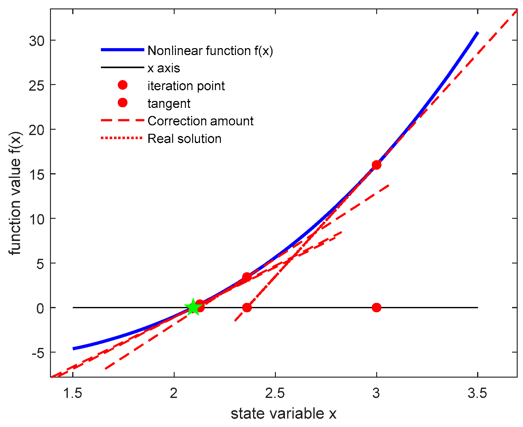
After solving, obtain the state variables to be solved, and substitute them as initial values into the node power equation. Form the required coefficient sequence for each iteration step into a matrix, and then use matrix operations to calculate the coefficients required for the next iteration step. Repeat the iterative calculation until the final solution that meets the accuracy is obtained, thus obtaining the power flow distribution. In this way, the power at each node can be obtained from the node power equation, and the power flow distribution of the power system can be obtained through the active power balance equation and reactive power balance equation. The principle is shown in the following diagram in Figure 2.

This method utilizes the local linear approximation of the function at the current point to rapidly update the root estimate. By iteratively approximating the curve with its tangent line and locating the root of this linear approximation, it progressively converges towards the true root of the function, as shown in Figure 2. The green pentagram represents the exact location of the solution.

2.3. Convergence in Newton Raphson Current Calculation

Through the principle analysis of the Newton-Raphson power flow algorithm above, it can be seen that the theory of this method is relatively simple and the calculation process is also relatively simple. However, in practical numerical simulations, convergence difficulties often occur.

Generally speaking, when using the Newton–Raphson algorithm for power flow calculation, only seven or more iterations are needed to achieve high accuracy. Although the number of iterations is proportional to the system size, the increase in iteration times is not significant as the power grid size increases. In the IEEE 30 bus example presented in this paper, the solution results that meet the error accuracy requirements were obtained. In theory, if the initial parameters given are accurate enough, then when using this algorithm for calculation, the error will decrease squared at the iteration point, exhibiting quadratic convergence.

However, if we choose inappropriate initial values with given parameters, we may experience non0convergence, or converge to a solution that does not match the actual situation. The non-convergence situation may result in the model not being able to accurately fit the data, and may even affect the performance of the model. Therefore, when selecting initial values, special attention should be paid to ensuring that the selected initial values are correct, to ensure that the model can accurately fit the data.

In general, we can assume that each effective initial value of a node is the rated voltage of the $PQ$ network, and after standardization, the initial voltage value is set to 1, and the initial values of the voltage phase angle is set to 0. This is because during normal system operation, the voltage at each node will not differ significantly from the rated voltage, and the voltage phase angle at each node is relatively close, which will not have a significant impact on the iteration results.

When conducting power flow calculations, attention should be paid to the multi-value nature of the power flow; that is, the results obtained for a given initial value are inconsistent. The reason for this situation is that the dynamic equation of the power system is a non-linear system, so theoretically it is impossible to have only one solution. However, the premise is that in the calculation of the power system, all non-real solutions must be eliminated.

In the above situations, there may be some solutions (or non-stationary solutions) that are not present in reality. There may also be some reasonable solutions that can be obtained in reality, but the operating voltage and power loss of these solutions may vary.

In contrast to the above situation, due to various reasons, the calculation of power flow may not converge, which can be referred to as “non-convergence”. We need to further analyze this situation to determine if it is due to the following reasons:

(a)

Improper network parameter settings;

(b)

Inaccurate parameters;

(c)

The algorithm is incorrect;

(d)

Initial value selection error;

(e)

The algorithm itself has flaws;

(f)

Other reasons.

It is worth noting that sometimes power flow calculations can converge and obtain real number solutions, but this does not mean that all of these solutions can be used as actual power flow results, for example in the following situations:

(a)

When the current flowing through the component exceeds its allowable value;

(b)

When the effective value of the node voltage exceeds the rated maximum value or falls below the minimum value;

(c)

When the power of a node exceeds its allowable value.

When the above situations occur, we need to adjust the following two points: ① the active power of the generator; ② the initial value of node voltage for node $PV$. In fact, when the reactive power of node $PV$ exceeds the allowable range of the generator, changing it to node $PQ$ can also improve the power flow calculation results.

Of course, improving the trend results requires vast experience and sufficient patience to constantly repeat and explore the process.

2.4. The Principle of P-Q Decomposition Method

The principle of P-Q decomposition method for the power system flow calculation is to transform the power system flow calculation problem into a solution problem in a linear equation system, and then use the solution method of the linear equation system to perform the power system flow calculation. The basic idea of P-Q decomposition method is to divide the power flow calculation problem into multiple parts and then solve them separately. Specifically, the first step of the P-Q decomposition method is to divide the power system into multiple linear equation systems, each of which contains several node voltage and power equations. The second step is to decompose each linear equation system into multiple independent sub-equation systems, each containing several node voltage and power equations. The third step is to use the solution method for the linear equation system to solve the power flow calculation problem in the power system; that is, to determine the solutions for the node voltage and power equations in each sub-equation system through iterative calculation. The advantages of the P-Q decomposition method are that it can greatly simplify the process of power flow calculation in power systems, and it can be widely applied in large-scale power flow calculation. However, the P-Q decomposition method also has some limitations, such as the need to handle non-linear systems and the long computation time, making it less practical in power system flow calculations that require fast computation.

The commonly used P-Q decomposition method in power systems is derived from the Newton–Raphson method represented in polar coordinates. Considering the characteristics of the power grid, the P-Q decomposition method is a simplification of the Newton–Raphson method for modifying equations [17]. Firstly, in the power grid, the reactance of each component is generally much greater than the resistance (X>>R), so the phase angle change of each node voltage has the greatest impact on the active power flow, while the amplitude change of each node voltage has the greatest impact on the reactive power flow. Therefore, subarrays $N,M$ can be omitted, and the modified equation becomes:

$$\left[\begin{array}{c}\Delta \stackrel{\rightharpoonup }{P}\\ \Delta \stackrel{\rightharpoonup }{Q}\end{array}\right]=\left[\begin{array}{cc}H& \\ & L\end{array}\right]\left[\begin{array}{c}\Delta \stackrel{\rightharpoonup }{\theta }\\ \Delta \stackrel{\rightharpoonup }{U}/U\end{array}\right]$$

(7)

The second simplification is based on the constraint condition $|{\theta }_i-{\theta }_j|<|{\theta }_i-{\theta }_j{|}_{\max }$ on state variable ${\theta }_i$, which means that $|{\theta }_i-{\theta }_j|={\theta }_{ij}$ should not be too large. Considering $G_{ij}<<B_{ij}$, it can be considered as $\cos {\theta }_{ij}\approx 1$, $G_{ij}\sin {\theta }_{ij}<<B_{ij}$, and $U_i^2{B}_{ii}>>Q_i$. Therefore, $H_{ij},L_{ij}$ can be simplified as:

$$H_{ij}=-U_i{U}_j{B}_{ij}$$

(8)

$$L_{ij}=-U_i{U}_j{B}_{ij}$$

(9)

So $H$ and $L$ can be expressed as:

$$H=-U{B}^{\prime }U$$

(10)

$$L=-U{B}^{″}U$$

(11)

$B^{\prime }$ and $B^{″}$ are constant matrices of order n − 1 and m − 1, respectively. Substitute the above equation into the equation and organize it to obtain

$$\Delta \stackrel{\rightharpoonup }{P}/U=-B^{\prime }(U\Delta \stackrel{\rightharpoonup }{\theta })$$

(12)

$$\Delta \stackrel{\rightharpoonup }{Q}/U=-B^{″}\Delta \stackrel{\rightharpoonup }{U}$$

(13)

In order to reduce the influence of reactive power and the node voltage modulus on active iteration during the iteration process, the elements in the right-hand end of the equation are set to a unit value of 1.0; that is, $U$ is the unit matrix.

The corrected equation for the commonly used fast decoupling algorithm can be written as:

$$\Delta \stackrel{\rightharpoonup }{P}/U=-B^{\prime }\Delta \stackrel{\rightharpoonup }{\theta }$$

(14)

$$\Delta \stackrel{\rightharpoonup }{Q}/U=-B^{″}\Delta \stackrel{\rightharpoonup }{U}$$

(15)

Node power is represented as a polar coordinate equation of the voltage vector. The active power error is used as the basis for correcting the angle of voltage vector, and the reactive power error as the basis for correcting voltage amplitude, iteratively separating active and reactive power. The main content of the P-Q decomposition method is to calculate the imbalance of node power using a formula, solve for correction factors $\Delta \theta$ and $\Delta \nu$ using a correction equation, and iterate until the power errors $\Delta P_i$ and $\Delta \nu$ of each node satisfy the convergence condition.

Its characteristics are:

-

Replace the original $2n-m-1$ linear equation system with a system of $n-1$ and $n-m-1$ linear equations;

-

The coefficient matrices $B^{\prime }$ and $B^{″}$ of the modified equation are symmetric constant matrices that remain unchanged during the iteration process;

-

It has linear convergence and requires more iterations to converge to the same accuracy compared to the Newton–Raphson method;

-

It is generally only applicable to the calculation of power grids with voltage levels of 110 KV and above. Due to the large ratio of lines with voltage levels of 35 KV and below, which does not meet the simplified conditions mentioned above, iterative calculations may not converge.

3. Simulation Operation and Its Results

A. 

Trend analysis operating environment

This trend analysis was run entirely in the Matlab2022b program environment. Figure 3 is a brief introduction to the simulation and use of this software. The figure shows the sub process analysis, and a further optimization matrix analysis is obtained by distinguishing the transformer branch and error boundary values.

Basic area: After opening the software, the software interface is divided into several areas, including the command function area at the top, the command line input bar on the right, and the currently opened folder and its path on the left. The middle is the workspace, which is also the area where our program design is located. We need to write the source code for the trend analysis and design program in this area. The specific implementation flowchart is as follows:

B. 

Comparison of Trend Analysis and Simulation Results

Import the results of the P-Q decomposition method and the Newton–Raphson method power flow calculation into an Excel spreadsheet and use Origin to draw a line graph. Visualize the node voltage amplitude, node voltage phase angle, node power, line power loss, branch injection power, and branch output power separately.

(1)

Analysis of Newton–Raphson Method Results

The reference capacity is 100 MVA and the reference voltage is Uav. The following data are all standard values. The calculation results for the Newton–Raphson method are as follows:

The first to fifth columns of

Table 1. IEEE 30 bus power flow distribution.

Node	Voltage Node	Phase Angle Node	Active Power Node	Node Reactive Power
1	1.060000	0.000000	1.669979	−0.006778
2	1.045000	−3.225387	0.183000	0.252103
3	1.022696	−5.680193	−0.024000	−0.012000
4	1.013861	−6.825930	−0.076000	−0.016000
5	1.010000	−6.345533	−0.094200	−0.141039
6	1.011154	−7.924344	0.000000	0.000000
7	1.001916	−7.814514	−0.228000	−0.109000
8	1.010000	−8.659255	−0.300000	0.046273
9	1.051657	−11.075883	0.000000	0.000000
10	1.046261	−12.722266	−0.058000	−0.020000
11	1.082000	−11.075883	0.000000	0.157839
12	1.057649	−12.218629	−0.112000	−0.075000
13	1.071000	−12.218629	0.000000	0.102139
14	1.042815	−13.077570	−0.062000	−0.016000
15	1.038444	−13.137198	−0.082000	−0.025000
16	1.045370	−12.694425	−0.035000	−0.018000
17	1.040937	−12.928725	−0.090000	−0.058000
18	1.029072	−13.684535	−0.032000	−0.009000
19	1.026654	−13.818447	−0.095000	−0.034000
20	1.030780	−13.601486	−0.022000	−0.007000
21	1.033859	−13.169275	−0.175000	−0.112000
22	1.034384	−13.156759	0.000000	0.000000
23	1.028070	−13.459859	−0.032000	−0.016000
24	1.022611	−13.544808	−0.087000	−0.067000
25	1.018495	−13.042317	0.000000	0.000000
26	1.000839	−13.461004	−0.035000	−0.023000
27	1.024460	−12.472177	0.000000	0.000000
28	1.007514	−8.554036	0.000000	0.000000
29	1.004647	−13.699154	−0.024000	−0.009000
30	0.993188	−14.579783	1.669979	−0.019000

are the node count, voltage amplitude (per unit value) of each node, phase angle (angle system) of the node voltage, active power inflow (per unit value) of each node, and reactive power inflow (per unit value) of each node, respectively. The first and second columns of the data in Appendix A,

Table A1. IEEE 30 bus branch power.

Node I	Node J	Active Power Branch	Reactive Power Branch	Active Loss Branch	Reactive Loss Branch
2	1	−1.047888	0.078981	0.019511	−0.000062
3	1	−0.587609	−0.055181	0.014971	0.017085
4	2	−0.396089	−0.058650	0.008787	−0.012229
4	3	−0.559571	−0.040298	0.004038	0.002883
5	2	−0.312549	−0.117301	0.004946	−0.023363
6	2	−0.494609	−0.030098	0.013908	0.002664
6	4	−0.454814	0.064555	0.002463	−0.000657
7	5	−0.216191	0.008535	0.002158	−0.015202
7	6	−0.011809	−0.117535	0.000320	−0.016241
8	6	−0.295143	0.053995	0.001065	−0.005464
6	9	0.287389	−0.304000	0.000000	0.035603
6	10	0.164241	−0.117839	0.000000	0.022220
11	9	0.000000	0.157839	0.000000	0.004426
10	9	−0.287389	−0.047198	0.000000	0.008523
4	12	0.422383	−0.459137	0.000000	0.096933
13	12	0.000000	0.102139	0.000000	0.001273
14	12	−0.075893	−0.023455	0.000714	0.001485
15	12	−0.168652	−0.066236	0.002015	0.003970
16	12	−0.062665	−0.034604	0.000443	0.000932
15	14	−0.013843	−0.007409	0.000051	0.000046
17	16	−0.027615	−0.016421	0.000050	0.000183
18	15	−0.055018	−0.016897	0.000336	0.000683
19	18	−0.022982	−0.007825	0.000036	0.000072
20	19	0.072207	0.026554	0.000189	0.000379
20	10	−0.094207	−0.033554	0.000881	0.001967
17	10	−0.062385	−0.041579	0.000168	0.000438
21	10	−0.157915	−0.097379	0.001121	0.002412
22	10	−0.076420	−0.044684	0.000532	0.001098
22	21	0.017091	0.014632	0.000005	0.000011
23	15	−0.044863	−0.030502	0.000278	0.000562
24	22	−0.058854	−0.029312	0.000475	0.000740
24	23	−0.012816	−0.014406	0.000047	0.000096
25	24	0.015457	−0.021463	0.000127	0.000222
26	25	−0.035000	−0.023000	0.000445	0.000665
27	25	0.051176	0.002725	0.000274	0.000522
28	27	0.183990	−0.122985	0.000000	0.019107
29	27	−0.061036	−0.015057	0.000861	0.001626
30	27	−0.069298	−0.013575	0.001619	0.003047
30	29	−0.036702	−0.005425	0.000335	0.000633
28	8	0.004871	−0.035787	0.000014	−0.043509
28	6	−0.188861	−0.013506	0.000595	−0.011136
10	0	0.000000	−0.207986	0.000000	−0.207986
24	0	0.000000	−0.044967	0.000000	−0.044967

represent two nodes with a connection relationship, the third and fourth columns show the power flow between the two nodes, and the fifth and fourth columns show the loss of active and reactive power in the line between the two nodes.

The first to fifth columns of Table 1 are the node count, voltage amplitude (per unit value) of each node, phase angle (angle system) of the node voltage, active power inflow (per unit value) of each node, and reactive power inflow (per unit value) of each node, respectively. The first and second columns of the data in Appendix A, Table A1 represent two nodes with a connection relationship, the third and fourth columns show the power flow between the two nodes, and the fifth and sixth columns show the loss of active and reactive power in the line between the two nodes.

(2)

Analysis of P-Q Decomposition Method Results

The reference capacity is 100 MVA and the reference voltage is Uav. The following data are all standard values. The calculation results for the P-Q decomposition method are as follows:

According to Appendix A,

Table A2. IEEE 30 bus power flow distribution (P-Q decomposition method).

Node	Type	Generator Active	Generator Reactive	Load Active	Load Reactive	Voltage Amplitude	Voltage Phase
1	1	2.609518	−0.165265	0.000000	0.000000	1.060000	0.000000
2	2	0.400000	0.495648	0.217000	0.127000	1.043000	−0.093375
3	3	0.000000	0.000000	0.024000	0.012000	1.020710	−0.131463
4	3	0.000000	0.000000	0.076000	0.016000	1.011726	−0.162045
5	2	0.000000	0.369360	0.942000	0.190000	1.010000	−0.247263
6	3	0.000000	0.000000	0.000000	0.000000	1.010231	−0.193127
7	3	0.000000	0.000000	0.228000	0.109000	1.002361	−0.224556
8	2	0.000000	0.372186	0.300000	0.300000	1.010000	−0.206203
9	3	0.000000	0.000000	0.000000	0.000000	1.050896	−0.246263
10	3	0.000000	0.000000	0.058000	0.020000	1.045109	−0.274027
11	2	0.000000	0.161798	0.000000	0.000000	1.082000	−0.246263
12	3	0.000000	0.000000	0.112000	0.075000	1.057104	−0.260824
13	2	0.000000	0.106306	0.000000	0.000000	1.071000	−0.260824
14	3	0.000000	0.000000	0.062000	0.016000	1.042265	−0.276396
15	3	0.000000	0.000000	0.082000	0.025000	1.037665	−0.278000
16	3	0.000000	0.000000	0.035000	0.018000	1.044373	−0.271001
17	3	0.000000	0.000000	0.090000	0.058000	1.039885	−0.276849
18	3	0.000000	0.000000	0.032000	0.009000	1.028136	−0.288723
19	3	0.000000	0.000000	0.095000	0.034000	1.025634	−0.291755
20	3	0.000000	0.000000	0.022000	0.007000	1.029720	−0.288325
21	3	0.000000	0.000000	0.175000	0.112000	1.032708	−0.281754
22	3	0.000000	0.000000	0.000000	0.000000	1.033239	−0.281505
23	3	0.000000	0.000000	0.032000	0.016000	1.027164	−0.284820
24	3	0.000000	0.000000	0.087000	0.067000	1.021564	−0.287902
25	3	0.000000	0.000000	0.000000	0.000000	1.017318	−0.280435
26	3	0.000000	0.000000	0.035000	0.023000	0.999640	−0.287760
27	3	0.000000	0.000000	0.000000	0.000000	1.023228	−0.271283
28	3	0.000000	0.000000	0.000000	0.000000	1.006797	−0.204017
29	3	0.000000	0.000000	0.024000	0.009000	1.003389	−0.292750
30	3	0.000000	0.000000	0.106000	0.019000	0.991914	−0.308159

, the results of calculating the power flow distribution of the IEEE 30 bus using the program ieee30-PQ.m include the number of nodes and node types, where 1 represents the balance node, 2 represents the PV node, and 3 represents the PQ node. It also includes the active and reactive power generated by the generator and the active and reactive power required by the load, as well as the phase angle of each node.

According to Appendix A,

Table A3. IEEE 30 bus branch power (P-Q decomposition method).

Input	Output	Input Active	Input Reactive	Input Charging	Output Active	Output Reactive	Output Charging
1	2	1.7322321	−0.1812633	0.0296630	1.6803961	−0.3365012	0.0282199
1	3	0.8772860	0.0685826	0.0229214	0.8461362	−0.0452658	0.0205233
2	4	0.4361960	0.0589676	0.0196684	0.4260444	0.0280319	0.0178536
3	4	0.8221362	−0.0316363	0.0042254	0.8135599	−0.0562606	0.0040753
2	5	0.8238561	0.0402509	0.0223407	0.7943364	−0.0837692	0.0187658
2	6	0.6033440	0.0247423	0.0199891	0.5838694	−0.0343517	0.0176786
4	6	0.7215428	−0.1589336	0.0043664	0.7151965	−0.1810124	0.0042542
5	7	−0.1476636	0.1273156	0.0091584	−0.1493777	0.1229929	0.0092319
6	7	0.3811909	−0.0210706	0.0080357	0.3773777	−0.0327813	0.0076933
6	8	0.2956783	−0.0768541	0.0042542	0.2945809	−0.0806950	0.0042056
6	9	0.2771755	−0.1945860	0.0000000	0.2771755	−0.2174466	0.0000000
6	10	0.1583628	−0.0589910	0.0000000	0.1583628	−0.0740673	0.0000000
9	11	0.0000000	−0.1571471	0.0000000	0.0000000	−0.1617982	0.0000000
9	10	0.2771755	0.0591379	0.0000000	0.2771755	0.0511374	0.0000000
4	12	0.4420616	−0.1705691	0.0000000	0.4420616	−0.2229015	0.0000000
12	13	0.0000000	−0.1049267	0.0000000	0.0000000	−0.1063060	0.0000000
12	14	0.0785910	0.0240122	0.0000000	0.0778471	0.0224657	0.0000000
12	15	0.1789784	0.0679586	0.0000000	0.1768071	0.0636816	0.0000000
12	16	0.0724921	0.0335389	0.0000000	0.0719525	0.0324044	0.0000000
14	15	0.0158528	0.0064714	0.0000000	0.0157931	0.0064175	0.0000000
16	17	0.0369525	0.0144044	0.0000000	0.0368769	0.0141270	0.0000000
15	18	0.0601978	0.0159756	0.0000000	0.0598112	0.0151884	0.0000000
18	19	0.0278113	0.0061884	0.0000000	0.0277622	0.0060892	0.0000000
19	20	−0.0672377	−0.0279108	0.0000000	−0.0674090	−0.0282534	0.0000000
10	20	0.0902243	0.0370740	0.0000000	0.0894090	0.0352534	0.0000000
10	17	0.0532653	0.0442439	0.0000000	0.0531231	0.0438729	0.0000000
10	21	0.1578620	0.1001202	0.0000000	0.1567486	0.0977240	0.0000000
10	22	0.0761869	0.0460076	0.0000000	0.0756597	0.0449205	0.0000000
21	22	−0.0182513	−0.0142760	0.0000000	−0.0182572	−0.0142879	0.0000000
15	23	0.0503964	0.0291176	0.0000000	0.0500818	0.0284821	0.0000000

, the line related parameters of the IEEE 30 bus power flow distribution include the active and reactive power flowing into the line, the active and reactive power flowing out of the line, and the part that includes reactive power compensation for the system by the ground branch.

(3)

Comparison of Calculation Time

The P-Q decomposition method took 0.066287 s to calculate the 30 node power flow distribution results in

Table 2. Comparison of calculation time.

Content	N-R	P-Q
Estimated time/s	0.143574	0.066287

. The Newton–Raphson method took 0.143574 s to calculate the distribution of 30 node currents.

After comprehensively comparing the power flow calculation results of the ex- tended model and the basic model in

Table 3. Index analysis.

Content	Base Models	Extended Models
Sum of squares of voltage deviations	0.039896	0.040799
Active power loss /pu	0.176331	0.083778

, the following conclusions can be drawn: The basic model performs better in terms of voltage quality, with a lower sum of squares of voltage deviation (0.039896) compared to the extended model (0.040799), indicating that the node voltage is closer to the ideal value. The extended model exhibits significant advantages in system efficiency, with a substantial reduction in total active power loss (52.5%) from the basic model (0.176331 pu) to 0.083778 pu. This model reduces the total active power loss to 0.083778 pu, achieving a 52.5% improvement in energy efficiency compared to the basic model (0.176331 pu). This breakthrough improvement directly translates into savings in grid operation costs.

The Newton–Raphson method is easy to understand and implement. The advantage of this method is that it has a fast calculation speed, can calculate a large number of numerical solutions in a very short time, and has high accuracy. It can obtain accurate calculation results through mathematical derivation. The disadvantage of the Newton–Raphson method is that it requires a significant amount of computational resources, but in practical engineering, the relevant parameters of each node in the power system can be measured in reality. Compared to the P-Q decomposition method, although it has a faster calculation speed, its calculation accuracy is not as good as the Newton–Raphson method. In comparison, the Newton–Raphson method has stronger practicality.

C. 

Visualization of trend analysis simulation results

Based on the Origin software, the trend distribution results are visualized. Origin is a mathematical analysis software mainly used for data processing, statistical analysis, and plotting. It integrates many advanced technologies, such as relational databases, graph data representation, algebraic operations, numerical computation, and data visualization. Origin also supports multiple languages, making it easy to integrate with other software to complete complex analysis tasks.

This section compares the visualization of power flow distribution obtained using the Newton–Raphson method and the P-Q decomposition method, and explores which algorithm is more in line with the actual situation.

(1)

Node data comparison

The following trend visualization is obtained by processing the voltage amplitudes of the nodes in Table 1 and Appendix A Table A1 through Origin2022. All data are per unit values.

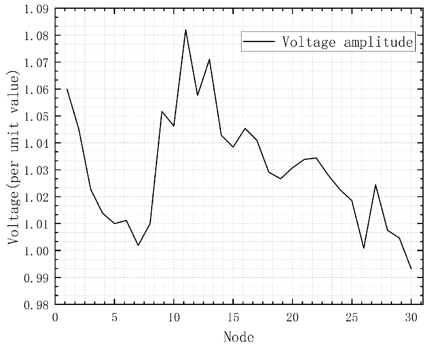
Figure 4 shows the voltage amplitude calculated by the Newton–Raphson method, The P-Q decomposition method is optimized by the Newton–Raphson method, and the node voltage amplitude results are consistent.

Therefore, both the Newton–Raphson method and the P-Q decomposition method can be used to solve the voltage amplitude in the power flow distribution of the power system network.

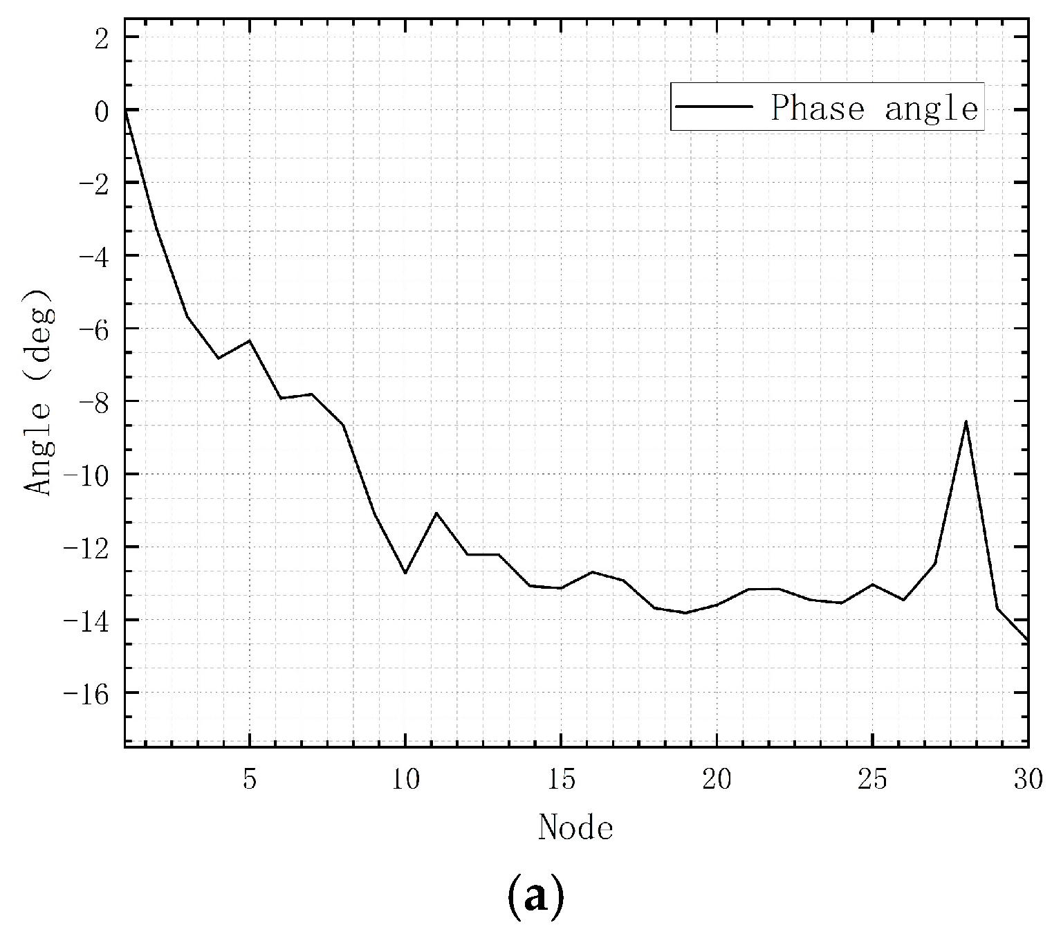
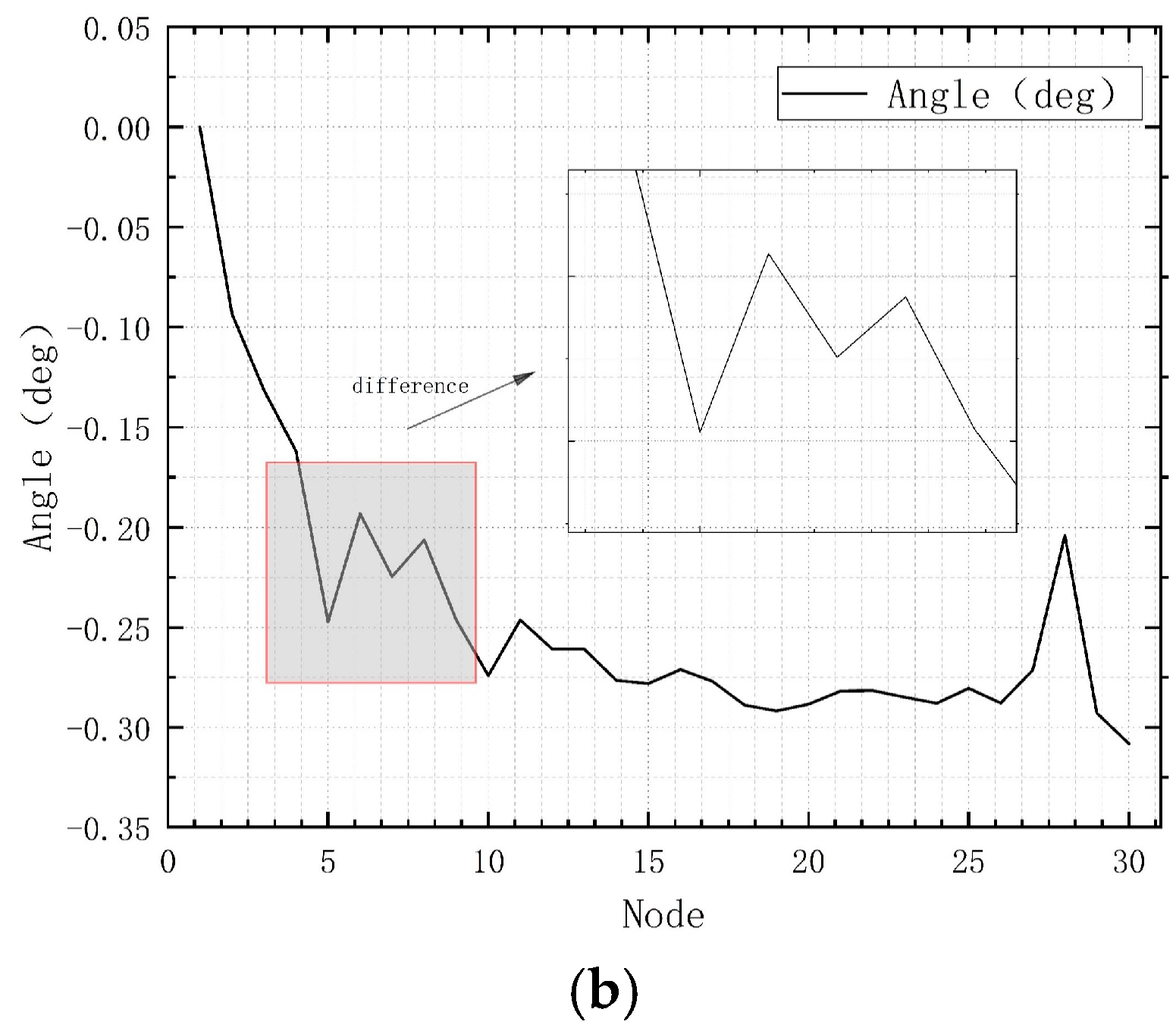
The voltage phase angles of the above nodes are all in radians. The Figure 5a shows the voltage phase angle calculated by the Newton–Raphson method, and Figure 5b shows the voltage phase angle calculated by the P-Q decomposition method, with local amplification processing applied to the highly differentiated intervals.

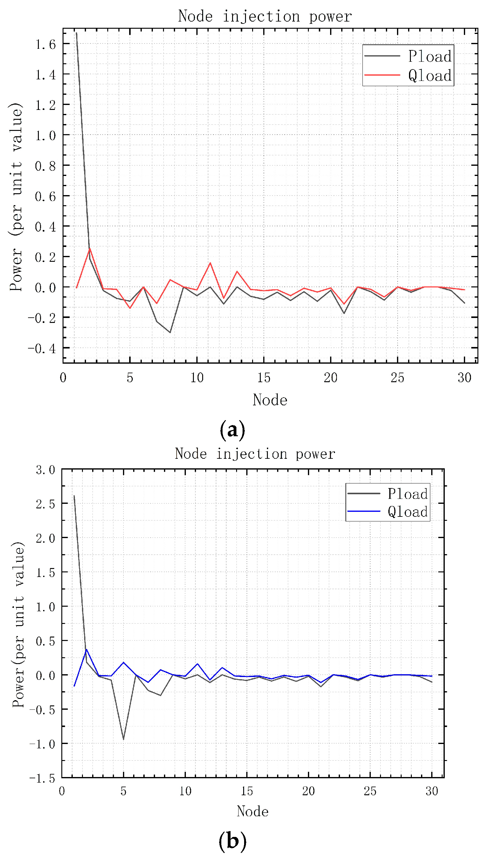
The above node powers are all per unit values. The Figure 6a shows the node power calculated by the Newton–Raphson method, and Figure 6b shows the node power calculated by the P-Q decomposition method.

It can be seen that the difference in node power calculated by the two currents is not significant.

(2)

Comparison of branch data

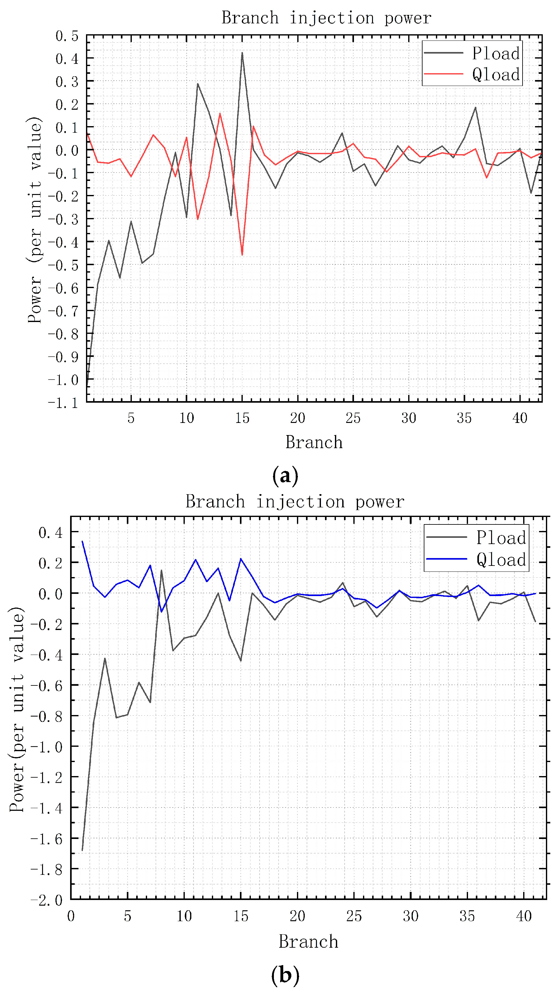
The above branch powers are all standard values. Figure 7a shows the branch injection power calculated by the Newton–Raphson method, and Figure 7b shows the branch injection power calculated by the P-Q decomposition method.

It can be seen that the difference in line power results calculated by the two power flow algorithms is not significant.

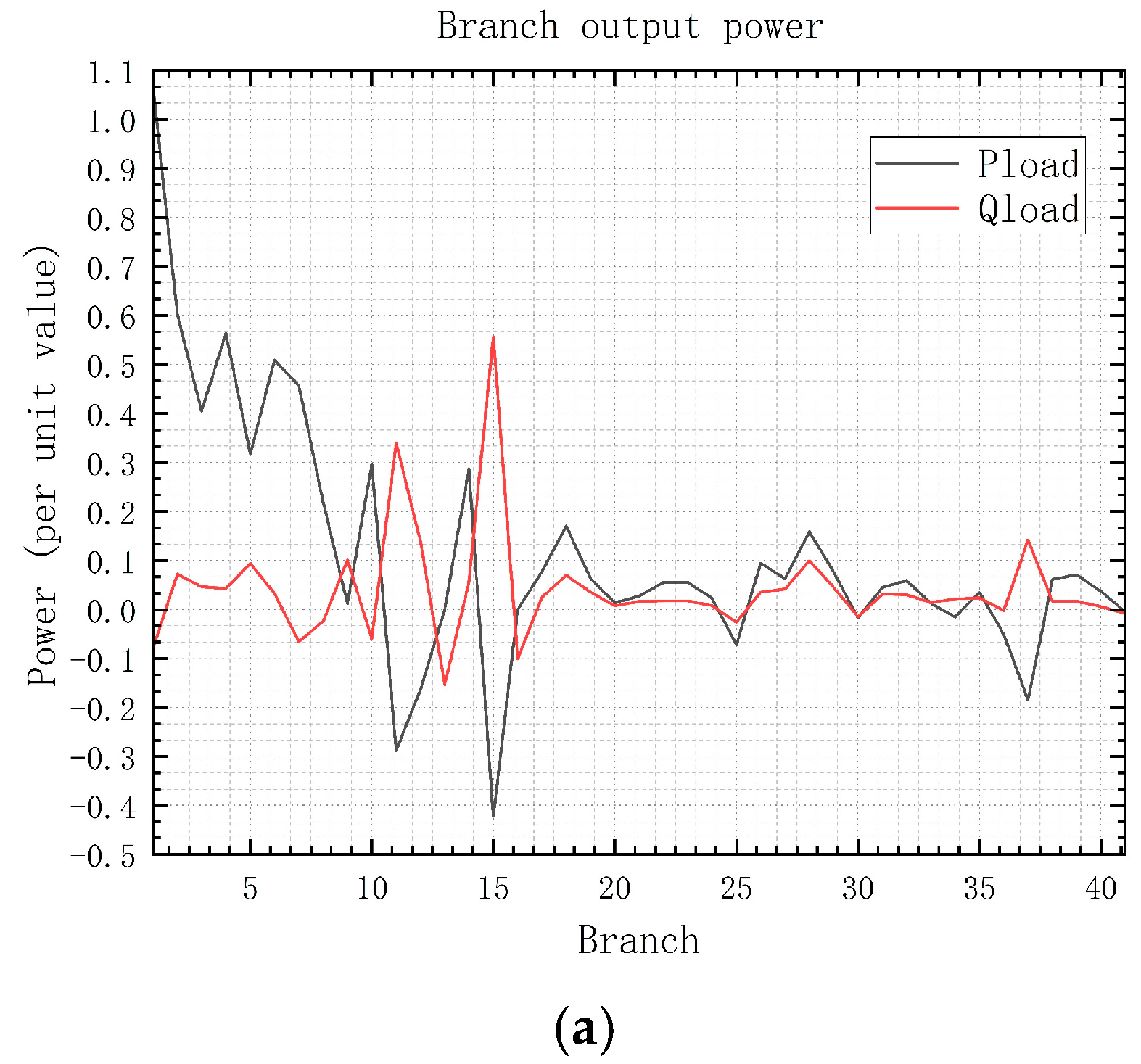
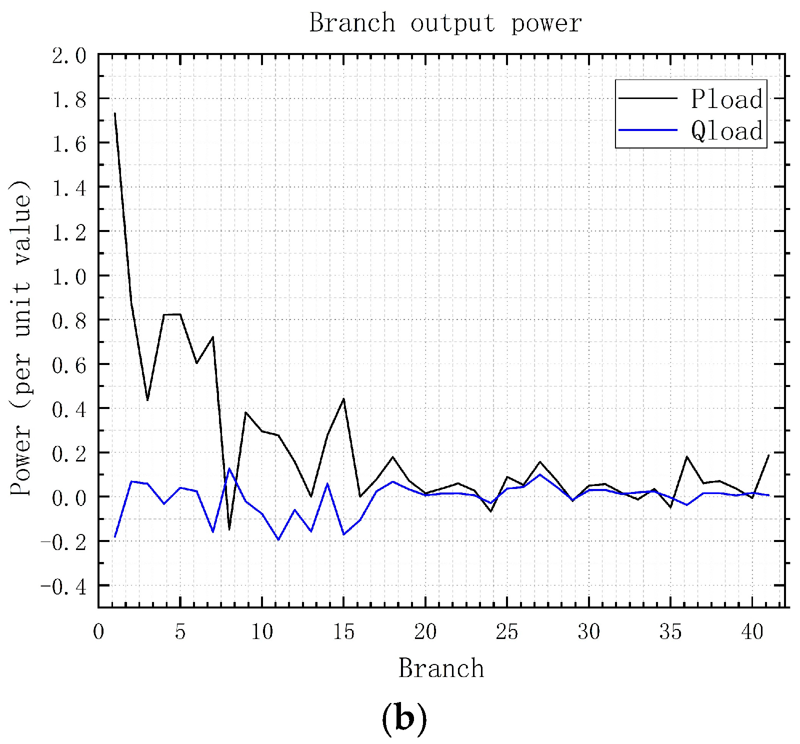
The above branch powers are all standard values. Figure 8a shows the branch output power calculated by the Newton–Raphson method, and Figure 8b shows the branch output power calculated by the P-Q decomposition method.

It can be seen that the difference in line power results is not significant.

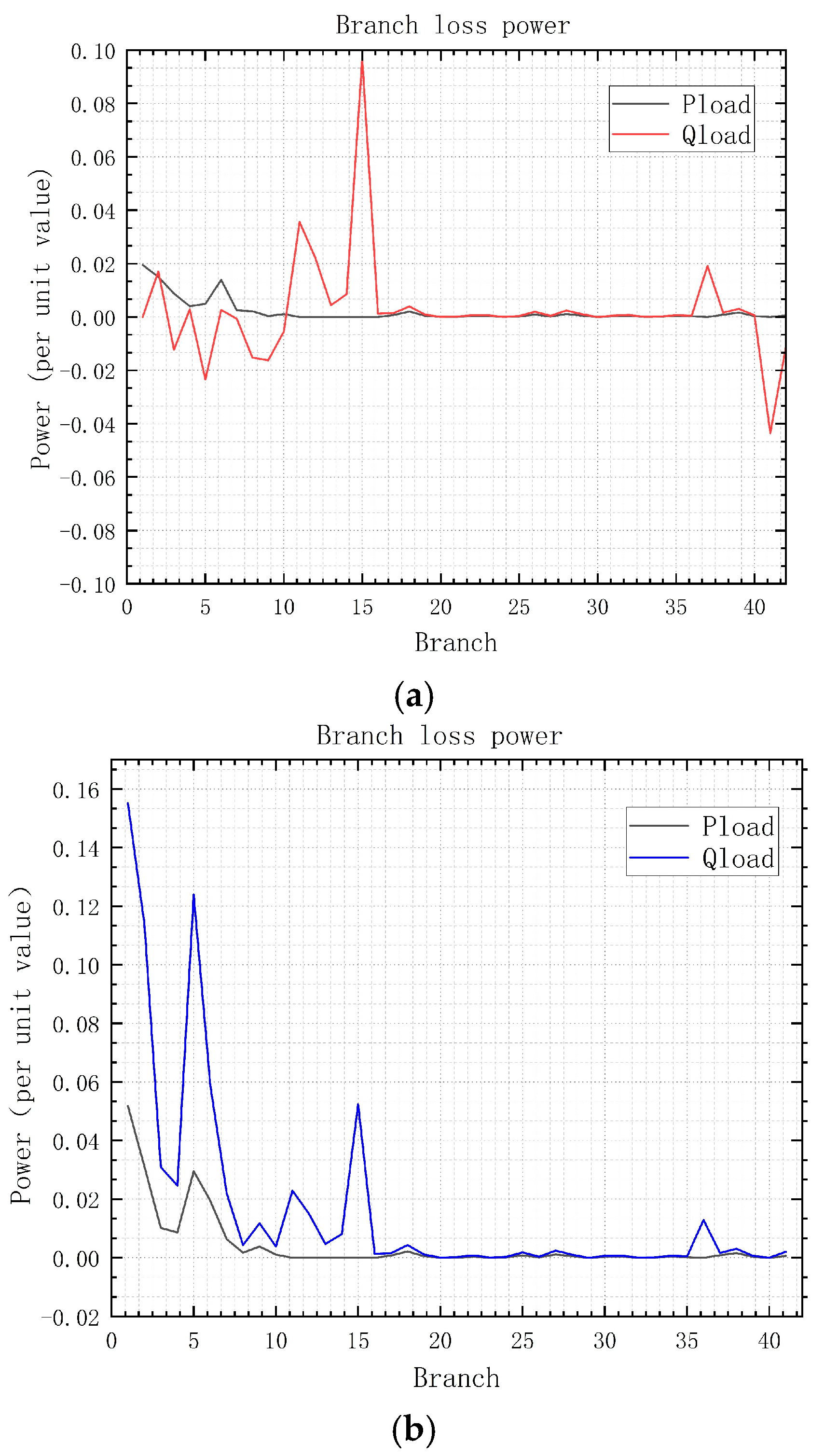
Figure 9a shows the branch power loss calculated by the Newton–Raphson method, and Figure 9b shows the branch power loss calculated by the P-Q decomposition method. It can be seen that the difference in the power loss results for the transmission lines is not significant, but there are still some subtle differences, because the P-Q decomposition method is only applicable to high-voltage transmission networks.

Due to the impedance X>>R of the transmission lines, active power and the voltage phase angles are strongly correlated, and reactive power and voltage amplitude are strongly correlated. Therefore, it can be simplified to consider only the bias of active power on the phase angle (active power has little effect on amplitude bias, simplified as a zero matrix), and the bias of reactive power on amplitude (reactive power has little effect on phase angle bias, simplified as a zero matrix). Neglecting the impact of resistance on line power and node voltage resulted in differences between the visualization of the power flow distribution and the Newton–Raphson method.

The voltage of the 30 node power system network flow distribution data visualization system is relatively stable, and there is basically no reactive power shortage. However, with the expansion of the power system and the significant increase in the number of nodes, combined with the flow distribution visualization results, it can be seen that a reactive power shortage has occurred. The phenomenon of reactive power loss control in multiple nodes requires the addition of reactive power compensation equipment. The location of the reactive power compensation device can be optimized and reconstructed based on the particle swarm optimization algorithm for the power system network.

Therefore, the calculation of power flow distribution in the power system is the basis for selecting appropriate reactive power compensation devices and reasonably planning the power grid structure.

4. Expansion of Trend Computing Model

With the widespread use of electricity, the scale of the power grid is constantly expanding and becoming increasingly complex. Therefore, considering the complex power flow distribution of large-scale power networks has become particularly important. This paper is based on the programming of example 030iee.dat to calculate its power flow distribution, and considers the complexity of the actual power system to extend the power flow calculation model to multiple nodes.

Change the 030ieee.dat data read from text read in the main program Untitled11.m to 057ieee.dat, 118ieee.dat, 162ieee.dat, and 300ieee.dat, respectively, to obtain different power flow distribution results. Use the openpyxl library in Python 3.11 to import the power flow calculation results into an Excel spreadsheet, and then use Origin 2022 drawing software to visualize the power flow distribution results.

A. 

IEEE 57 bus power flow distribution

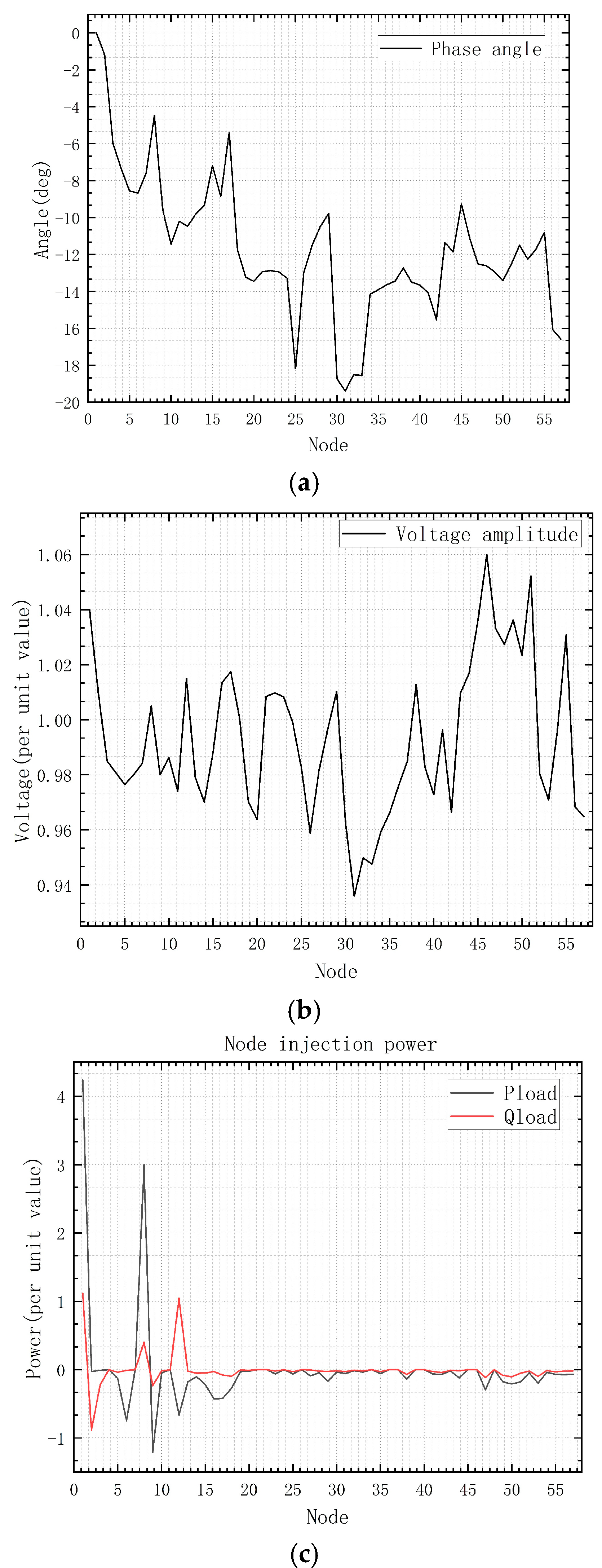
Change the 030iee.dat data read from text read in the main program Untitled11.m to 057iee.dat, run and visualize the power flow distribution. The results of the system operation are shown in Figure 10a–c and Figure 11a–c.

(1)

Node Data

Here is the final trend visualization:

Figure 10. (a) 57 bus voltage phase angle. (b) 57 bus voltage amplitude. (c) 57 bus node power.

Figure 10. (a) 57 bus voltage phase angle. (b) 57 bus voltage amplitude. (c) 57 bus node power.

(2)

Branch Data

Figure 11. (a) 57 bus branch inflow power. (b) 57 bus branch output power. (c) 57 bus branch power loss.

Figure 11. (a) 57 bus branch inflow power. (b) 57 bus branch output power. (c) 57 bus branch power loss.

B. 

ieee118bus power current distribution

Change the 030iee.dat data read by textread in the main program Untitled11.m to 118iee.dat, and run and visualize the power flow distribution. The results of the system operation are shown in Figure 12a–c and Figure 13a–c.

(1)

Node Data

Due to space limitations, only the final trend visualization is provided here.

Figure 12. (a) 118 bus voltage phase angle. (b) 118 bus voltage amplitude. (c) 118 bus node power.

Figure 12. (a) 118 bus voltage phase angle. (b) 118 bus voltage amplitude. (c) 118 bus node power.

(2)

Branch Data

Figure 13. (a) 118 bus branch inflow power. (b) 118 bus branch output power. (c) 118 bus branch power loss.

Figure 13. (a) 118 bus branch inflow power. (b) 118 bus branch output power. (c) 118 bus branch power loss.

C. 

IEEE 162bus power flow distribution

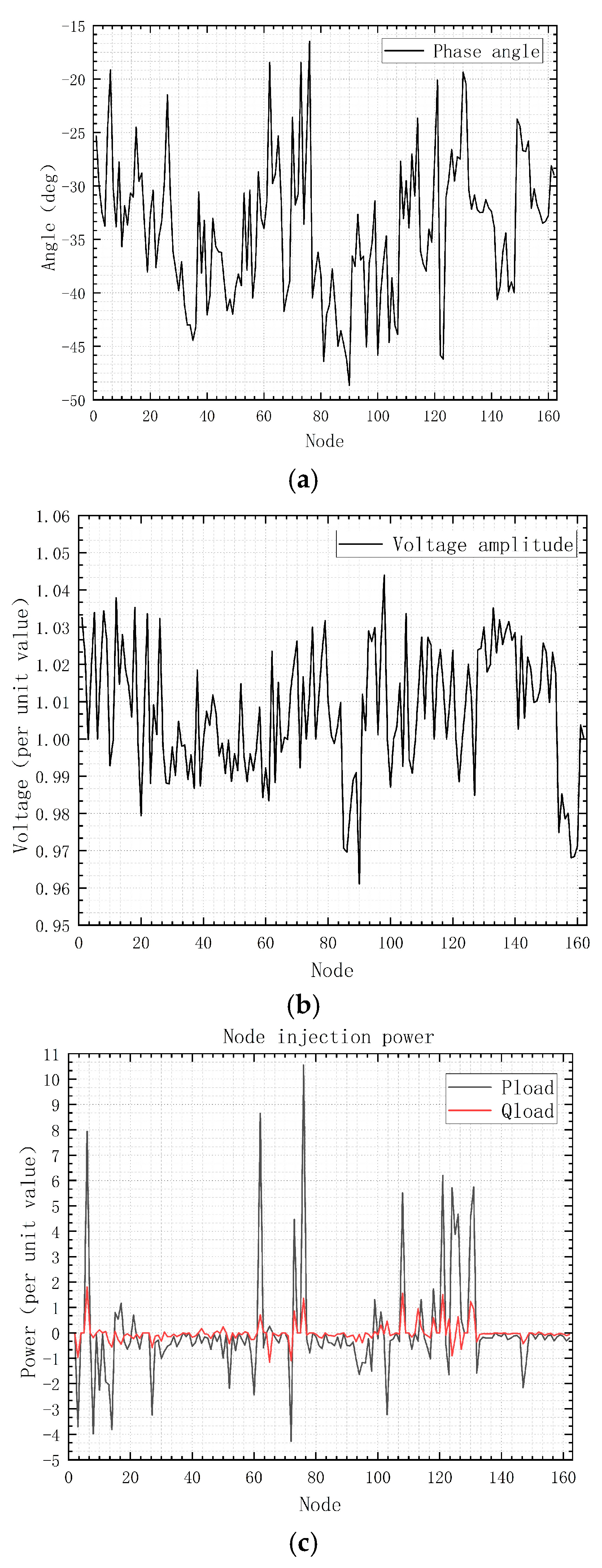
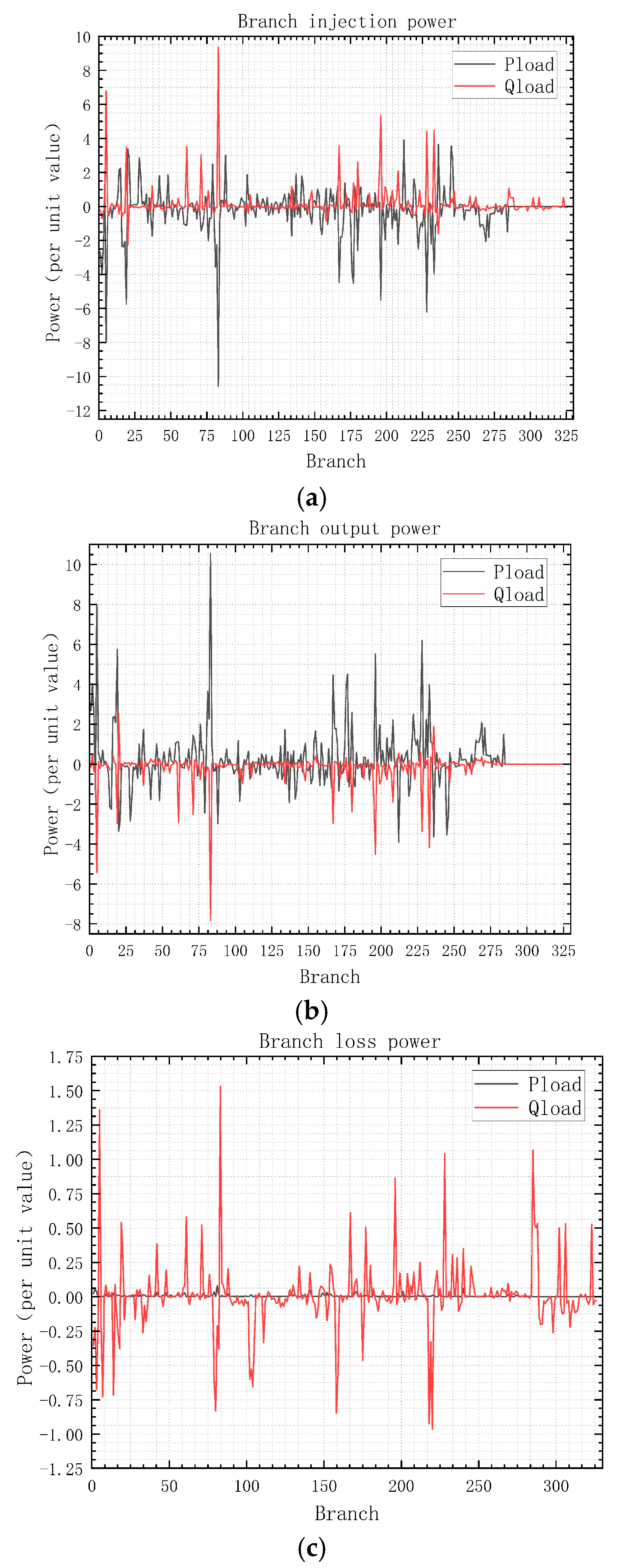
Change the 030iee.dat data read by textread in the main program Untitled11.m to 162iee.dat, and run and visualize the power flow distribution. The results of the system operation are shown in Figure 14a–c and Figure 15a–c.

(1)

Node Data

Due to space limitations, only the final trend visualization is provided here.

Figure 14. (a) 162 bus voltage phase angle. (b) 162 bus voltage amplitude. (c) 162 bus node power.

Figure 14. (a) 162 bus voltage phase angle. (b) 162 bus voltage amplitude. (c) 162 bus node power.

(2)

Branch Data

Figure 15. (a) 162 bus branch inflow power. (b) 162 bus branch output power. (c) 162 bus branch power loss.

Figure 15. (a) 162 bus branch inflow power. (b) 162 bus branch output power. (c) 162 bus branch power loss.

D. 

IEEE 300 bus power flow distribution

Change the 030iee.dat data read by textread in the main program Untitled11.m to 300iee.dat, and run and visualize the power flow distribution. The results of the system operation are shown in Figure 16a–c and Figure 17a–c.

(1)

Node Data

Here is the final trend visualization:

Figure 16. (a) 300 bus voltage phase angle. (b) 300 bus voltage amplitude. (c) 300 bus node power.

Figure 16. (a) 300 bus voltage phase angle. (b) 300 bus voltage amplitude. (c) 300 bus node power.

(2)

Branch Data

Figure 17. (a) 300 bus branch inflow power. (b) 300 bus branch output power. (c) 300 bus branch power loss.

Figure 17. (a) 300 bus branch inflow power. (b) 300 bus branch output power. (c) 300 bus branch power loss.

The voltage of the 30 node power system network flow distribution data visualization system is relatively stable, and there is basically no reactive power shortage in Figure 16a–c and Figure 17a–c. With the expansion of the power system and the significant increase in the number of nodes, combined with the flow distribution visualization results, it can be seen that a reactive power shortage has occurred. The phenomenon of reactive power loss control in multiple nodes requires the addition of reactive power compensation equipment. The location of the reactive power compensation device can be optimized and reconstructed based on the particle swarm optimization algorithm for the power system network.

Therefore, the calculation of power flow distribution in the power system is the basis for selecting appropriate reactive power compensation devices and reasonably planning the power grid structure.

5. Conclusions

(1)

Considering the complexity of actual power systems, a non-linear equation analysis is conducted to calculate the complex power flow iteration of multi-node power systems. The Newton–Raphson power flow calculation model is optimized and the power flow distribution of each complex power network is obtained, thus verifying the universality of the program.

(2)

The phenomenon of reactive power loss control occurs in multiple nodes, and it is necessary to add reactive power compensation equipment. Based on the particle swarm optimization algorithm, the optimal reconstruction of the power system network should be carried out for the location of the reactive power compensation device.

(3)

For the new optimization algorithm based on multi-radiation power grid optimization in the evolution process, it greatly reduces dependence on optimization time and initial state reconstruction, which provides novel ideas and references for complex non-linear systems.

When using Newton–Raphson power flow to calculate complex power systems, it is found that this method has a fast iteration speed and good convergence in power flow calculation. However, it is worth noting that when the determinant of the Jacobian matrix is small and the system parameters are low, it may lead to the inability of power flow calculation iterations to converge. In this case, we can use multiple power flow calculation methods to compare or combine two or more power flow methods to calculate the power grid.

The extended model exhibits significant advantages in system efficiency. This is a breakthrough improvement that directly translates into savings in grid operation costs.

With the development of technology and research into problems, the prospects for the development of reconstruction technology for complex power systems will be even broader. The current problems will be easily solved, thereby ensuring the continuity, reliability, and stability of the system.