Abstract
Traditional hydraulic-fracturing models are restricted by low computational efficiency, insufficient field data, and complex physical mechanisms, causing evaluation delays and failing to meet practical engineering needs. To address these challenges, this study innovatively develops a dynamic hydraulic-fracturing monitoring method that integrates machine learning with numerical simulation. Firstly, this study uses GOHFER 9.5.6 software to generate 12,000 sets of fracture geometry data and constructs a big dataset for hydraulic fracturing. In order to improve the efficiency of the simulation, a macro command is used in combination with a Python 3.11 code to achieve the automation of the simulation process, thereby expanding the data samples for the surrogate model. On this basis, a parameter sensitivity analysis is carried out to identify key input parameters, such as reservoir parameters and fracturing fluid properties, that significantly affect fracture geometry. Next, a neural-network surrogate model is established, which takes fracturing geological parameters and pumping parameters as inputs and fracture geometric parameters as outputs. Data are preprocessed using the min–max normalization method. A neural-network structure with two hidden layers is chosen, and the model is trained with the Adam optimizer to improve its predictive accuracy. The experimental results show that the efficiency of automated numerical simulation for hydraulic fracturing is significantly improved. The surrogate model achieved a prediction accuracy of over 90% and a response time of less than 10 s, representing a substantial efficiency improvement compared to traditional fracturing models. Through these technical approaches, this study not only enhances the effectiveness of fracturing but also provides a new, efficient, and accurate solution for oilfield fracturing operations.
1. Introduction
Fracturing stimulation is a crucial method for reducing costs and increasing production in oil fields [1]. Traditional fracturing stimulation requires a clear understanding of the fracture propagation mechanism and requires a large amount of oilfield data, which will limit the effect of fracturing stimulation [2,3]. Fracturing effect evaluation provides a direct understanding of the effectiveness of fracturing treatments and verifies whether the actual results align with design expectations. Numerical simulations using commercial software can make up for the lack of field data. Integrating artificial intelligence algorithms can build surrogate models to monitor and evaluate fracturing effects. This solves the timeliness problems of traditional models and provides better guidance for on-site operations.
Currently, real-time fracturing evaluation is gaining increasing attention in field applications. In light of the characteristics of unconventional reservoirs, research is underway in areas such as microseismic monitoring, fracturing parameter optimization, and reservoir response analysis. Furthermore, the application of artificial intelligence in real-time hydraulic-fracturing evaluation is also gaining increasing attention [4,5,6,7,8,9]. Traditional evaluation methods primarily compare geological exploration-predicted production with actual production after fracturing [10,11]. However, due to the lack of effective quantitative evaluation tools for fracturing effectiveness, the reasons for the discrepancy between predicted and actual production remain unclear. Furthermore, under complex construction conditions, existing evaluation methods are less timely and cannot adjust pumping parameters in real time during construction, resulting in suboptimal fracturing results.
The field of real-time hydraulic-fracturing assessment currently faces two major challenges: first, the complex physical mechanisms of the fracturing process result in inefficient computational models, making them incapable of meeting practical requirements [12,13,14], and second, limited field data (the small-sample-size problem) restricts the training of machine learning models [15,16,17,18,19,20]. With advances in artificial intelligence, emerging technologies such as cloud-based real-time fracturing assessment and machine learning-driven wellhead pressure prediction offer solutions to these problems [21,22,23,24,25]. They can be effectively addressed by simulating formation fracturing using numerical simulation methods, extracting fracturing simulation data using Python scripts, and combining time-series data analysis methods such as wavelet transforms to extract pumping time-series characteristics and construct a surrogate model for fracture propagation.
In tight oil and gas development, multi-stage fracturing significantly improves operational efficiency and reduces development costs. Monitoring fluid return rates and oil and gas production at different stages after fracturing is crucial. However, accurately characterizing the fracture network after fracturing in tight reservoirs remains a difficulty in field practice, directly impacting the accuracy of production performance predictions and fracturing effectiveness evaluations. Common characterization methods include microseismic event monitoring, production dynamic analysis, fracturing tracer backflow analysis, and monitoring using distributed optical fiber [26,27,28,29]. With the rapid digitalization and intelligent transformation of the oil and gas industry, integrating these technologies to improve the efficiency and quality of volume fracturing has become urgent. Current post-fracturing evaluations are typically conducted after construction, lacking the real-time capability to guide in-process parameter adjustments. Additionally, existing evaluation methods operate independently without mutual validation, limiting their comprehensiveness and accuracy. Consequently, there is an urgent need to develop an integrated real-time evaluation technology that combines real-time diagnostics, pressure decline analysis, and fracture network inversion to achieve comprehensive real-time assessment throughout the fracturing process. In this context, numerous scholars, both domestically and internationally, have carried out extensive research on post-fracturing stimulated reservoir volume (SRV) evaluation using production forecasting models, conducting in-depth analysis of the practical efficacy of fracture networks [30,31,32,33,34,35,36,37,38].
Therefore, this paper develops an integrated intelligent algorithm based on historical production data from domestic reservoirs, offering a novel approach to addressing bottlenecks in traditional hydraulic-fracturing assessment such as low computational efficiency, insufficient field data, and poor real-time performance. By utilizing GOHFER software to automatically generate large-scale fracture geometry data, combined with parameter sensitivity analysis to screen key influencing factors, and constructing a neural network-based proxy model, rapid and dynamic prediction of fracture propagation is achieved. Ultimately, a highly efficient, accurate, and real-time intelligent fracturing evaluation method is developed, providing scientific support for fracturing design optimization and field construction decision-making in unconventional oil and gas reservoirs and promoting the digital and intelligent development of fracturing technology.
This paper is organized as follows. Section 2 introduces the geological data and governing equations for the numerical simulation. Section 3 describes the method for generating a large dataset using GOHFER simulations, building a proxy model, and extracting pumping characteristics. Section 4 presents the results and compares the proxy model with a traditional model. Section 5 discusses and analyzes the results, and Section 6 concludes.
2. Governing Equations
This study is based on field data from the Ma-2 well block of the Mabei Oilfield, located on the northwestern margin of the Junggar Basin, approximately 110 km from Karamay City in Xinjiang, China. The parameter ranges used for numerical simulation were determined according to actual field application conditions, with specific values detailed in Section 4.1. The target reservoir is the Baikouquan Formation, which consists of a lithologic-structural trap bounded by major faults and characterized by low-amplitude anticlinal and nose-shaped uplifts favorable for hydrocarbon accumulation. The formation is divided into three submembers (T1b1, T1b2, T1b3), with productive intervals mainly located in T1b1 and T1b2.
The average formation thickness is about 135 m. The reservoir exhibits typical tight reservoir characteristics, with porosity ranging from 3.97% to 14.73% (average: ~8.0%) and permeability from 0.01 to 337 mD (average: ~0.5 mD). It is a low-saturation, abnormally high-pressure oil reservoir with an average pressure of 52.33 MPa and a formation temperature of 83.78 °C. The main oil-bearing layer (T1b22) has an average effective thickness of 18.4 m. The crude oil is a normal black oil with a density of 0.825 g/cm3 and viscosity of 5.65 mPa·s under surface conditions. The reservoir fluid contains a high proportion of methane (over 80%), and the formation water is NaHCO3-type, with an average salinity of 9848 mg/L and pH of 6.1.
The reservoir has weak-to-moderate sensitivity to water and salinity and low acid sensitivity. Natural fractures have not been developed, but interlayers and baffles composed of mudstone and argillaceous sandstone are present, which may affect vertical fluid flow and fracture propagation during hydraulic fracturing.
In conventional fracturing software, the linear elastic deformation mechanism is often adopted, which frequently results in predicted fracture widths exceeding actual measurements [39,40]. The GOHER 9.5.6 fracturing simulation software employs a shear–slip decoupling rock-fracturing mechanism, which aligns more closely with conventional fracturing practices [41]. The rock-fracturing mechanism of the rock is shown in Figure 1.
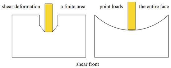
Figure 1.
Schematic diagram of rock-breaking mechanism.
The mechanism of the numerical simulation calculation of fracture length by this software is to estimate fracture flow length using the average conductivity, production length, and average permeability of the model grid. The calculation formula is as follows:
where is the fracture flow length, is the producing length, is the wellbore radius, is the fracture permeability, is the fracture width, and is the reservoir permeability.
The process zone stress (PZS) [42] is used as the fracture propagation criterion instead of fracture toughness. Stress distribution in rocks is not uniform; instead, the stress within the process zone remains nearly constant, termed the PZS. This criterion better reflects real-world conditions. The area of the process zone is given by
where is the process zone area, is the tensile strength of the material, and is the stress intensity f factor.
The tensile strength formula incorporating the process zone is
where is the apparent tensile strength, is the net closure stress, is the material tensile strength, and is the length of the fluid lag zone.
The FLIC leak-off model [43] is adopted instead of classical leak-off models. The FLIC model accounts for reservoir fluid compressibility and flow, non-Newtonian filtrate invasion, filter cake deposition, and equilibrium between filter cake thickness and fluid shear stress, thereby better simulating real leak-off behavior. The general solution of the FLIC model is
where is the total pressure drop, is the fluid loss volume, is the filtrate invasion rate in the invaded zone, is a constant for the non-invaded region, is a constant for the mixed zone, is the flow regime index, is the flow regime index, is a constant for the dynamic equilibrium zone, is the compressibility constant, and is the pressure drop measured under reference conditions.
The GOHFER software incorporates more realistic physical assumptions into its numerical simulations, including a shear–slip decoupled fracturing mechanism, the PZS fracture criterion, and the FLIC leak-off model. Compared to traditional approaches based on linear elasticity and classical leak-off models, these features enable more accurate simulation of fracture propagation, pressure response, and fluid flow behavior. By accounting for non-uniform stress distribution in the rock, fracture slip, and non-Newtonian filtrate invasion effects, GOHFER significantly enhances the physical consistency and accuracy of simulation results, providing a reliable data foundation for subsequent productivity forecasting, sensitivity analysis, and proxy model development.
3. Methodology
3.1. Automated Batch Simulation for Building a Hydraulic-Fracturing Big Dataset
The limited training sample size is a practical issue in oilfields. To solve the small-sample problem, especially when field datasets could not be expanded, we used hydraulic fracturing-software simulations. This allowed us to generate a big dataset. These datasets include fracture geometries and production outcomes under different geological and engineering parameters. This approach overcomes the limitations posed by insufficient field data.
In the field of intelligent prediction and optimization design for fracturing effects, vast amounts of completion and fracturing data have been digitized, providing a foundation for big-data analysis. However, fracturing data is diverse, voluminous, structurally complex, and sourced from multiple origins. To efficiently and accurately train models for predicting fracturing effects and optimizing designs, it is essential to first establish a high-quality dataset of engineering–geological data for hydraulic fracturing.
Hydraulic-fracturing engineering data primarily includes four categories: perforation data, fracturing fluid data, proppant data, and pumping protocol data. Perforation data includes parameters such as perforation cluster position selection, bridge plug location, number of clusters per interval, cluster spacing, cluster length, perforation density, phase angle, hole diameter, and perforation gun type. Fracturing fluid data includes parameters for friction-reducing water, gel fluid, and acid fluid. Proppant data includes usage data for proppants of different mesh sizes. Pumping protocol data includes parameters such as opening pressure, acid reduction pressure, breakdown pressure, operating pressure, shut-off pressure, staged pressure adjustment methods, flow rate, sand injection methods, and ball-landing plug data.
Figure 2 shows the parameter changes simulated during the pumping process based on the schedule. This figure mainly illustrates the schematic diagram of simulating pump injection using commercial software. The primary process for constructing the dataset is through simulating the pump-injection process with commercial software, then quickly extracting construction data using artificial intelligence technology and, finally, building a comprehensive big dataset based on the data and stage information.
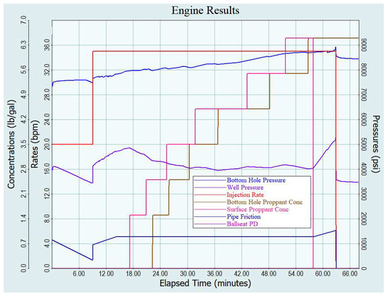
Figure 2.
Simulation of pump-injection program.
This section establishes a method for batch automation of fracturing-software simulations. Since commercial fracturing software typically lacks interfaces for automated batch processing, we utilized macro commands and Python scripts to automate the simulations. By using fracturing design software to simulate fracture geometries, we generated 12,000 groups of fracture geometric-parameter data to form a big dataset for machine-learning training. GOHFER software was selected for the simulations due to its ability to construct planar 3D fracture propagation models based on well logs, incorporating geological layering and inter-stage interference. It uses process zone stress (PZS) as the fracture propagation criterion, accounting for fluid lag, rock strength, and nonlinear stress dissipation at fracture tips, thereby effectively limiting fracture height growth. The fracturing simulation workflow begins with geological model construction based on well-logging data, followed by setting up a production-well model. During simulation execution, pumping design parameters are input to simulate fracturing while accounting for geological heterogeneity and inter-cluster interference. Finally, output parameters such as stimulated area per fracturing stage, fracture geometry, and production performance are obtained.
Figure 3a shows the wellbore trajectory of the fracturing well. Figure 3b indicates that as the well depth increases, the lithology of the formation changes continuously, and the geological parameters also change accordingly. This shows that the fracturing simulation performed by the GOHFER software is consistent with the actual complex geological conditions. Figure 3c uses fracture width as an example to show the changes in fracture morphology after fracturing. The fracture width is the largest near the wellbore, which is also consistent with the actual fracturing effect. We used macro commands to achieve automatic batch simulation of this process.
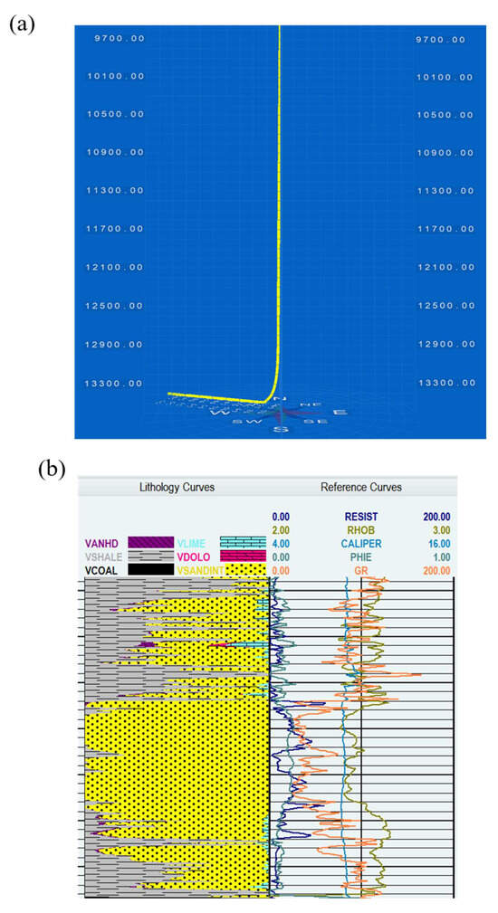
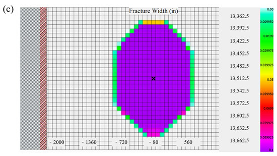
Figure 3.
Hydraulic-fracturing simulation: a and b show the geological model built based on well-logging data. (a) shows the wellbore trajectory of the built well model, and (b) shows the geological profile of the reference well, displaying geological parameters and formation lithology, with different-colored lines representing different parameters. Based on the built model, the software simulates the fracturing–pumping process, generating the image shown in (c), which shows the distribution of proppant in the fracture after fracturing, i.e., the fracturing effect. The center x in the figure is a horizontal wellbore, and the changes in different colors represent the changes in fracture width.
Macro commands are simple programs or scripts that can be executed within software, often designed to perform specific functions. By writing and applying macro commands, frequently used operations can be serialized, allowing multiple steps to be completed with a single macro execution. This is exemplified in fracturing software by automatically setting model parameters for different conditions, initiating simulations, and automatically saving simulation results. While macro commands can improve data generation efficiency to a certain extent, they cannot dynamically adjust simulation parameters and workflows as a project progresses to meet evolving research needs. Therefore, combining Python with macro commands is necessary to achieve more flexible automation. Python can be used to batch-modify numerical simulation input parameters and process simulated data, including extracting key parameters, data cleaning, format conversion, and statistical analysis, to prepare high-quality datasets for subsequent model training. In summary, by integrating Python code into fracturing software, macro commands can be called from Python to run multiple simulations with different parameter combinations, automatically recording the results of each simulation and enabling batch automation.
The automated workflow is systematically implemented through the following steps:
Identification and preprocessing of input/output files: First, locate the input and output files required for hydraulic-fracturing simulations by searching for keywords such as fracturing simulation, input, or output in the file system. Python scripts are then used to read the data and store it in structured containers, ensuring readiness for subsequent processing.
Automated parameter file modification: Python scripts are utilized to systematically modify various parameter files related to well logging, perforation, pumping protocols, and production. For well-logging parameters, adjustments are made to well depth, lithology, and other relevant parameters based on updated geological exploration data. In terms of perforation parameters, modifications are carried out on perforation layer counts and hole diameters. Pumping protocol parameters are updated to include changes to fluid formulations such as friction-reducing water and gel fluids, as well as adjustments to injection rates. Production parameters are revised to reflect updated production forecasts and pressure dynamics. This automated process ensures the rapid generation of parameter files that meet simulation requirements, thereby guaranteeing data accuracy and reliability for subsequent fracturing simulations.
Macro-driven automation of GOHFER simulations: A macro script is developed to fully automate the execution of the GOHFER software operations, which enhances efficiency and computational accuracy while minimizing human error. The script automates software initialization by launching GOHFER and navigating to the required module without manual intervention, executes simulations by inputting predefined parameters and processing data, and generates results by outputting them to designated locations.
Post-simulation data extraction and structuring: After the simulations are completed, Python scripts are employed to extract critical data from output files. The scripts first locate the result file paths, then use Python’s open function along with regular expressions to parse and isolate key parameters such as pumping data, fracture geometry, and production rates. The extracted data is subsequently stored in arrays or lists for subsequent analysis and visualization. This structured method ensures efficient use of simulation results and contributes to building a robust hydraulic-fracturing big dataset.
3.2. Parameter Sensitivity Analysis
Given the complexity of GOHFER simulations—requiring over 70 input parameters, including logging, reservoir, perforation, pumping, and production data—a sensitivity analysis was conducted to identify the critical parameters. This ensured the neural-network surrogate model was trained on high-impact features, improving precision.
Figure 4 illustrates the geological profile generated by the software based on the input logging data. It demonstrates that the geological input parameters are not only diverse in type but also vary significantly with depth, adding complexity to the data input process. Table 1 presents the pumping schedule used for numerical simulation, which includes parameters such as pumping time, fracturing fluid, and proppant properties. This table serves as an example—actual pumping schedules used in simulations are typically far more complex. GOHFER allows the design of sophisticated pumping programs to closely simulate real field operations. Table 2 lists the production parameters required for post-simulation production forecasting. Setting these parameters is critical for accurately predicting post-fracturing production. Collectively, these figures and tables represent the primary input parameters of the numerical simulation. Through the integrated design of geological parameters, pumping schedules, and production parameters, the software can effectively simulate the complex fracturing process in real field scenarios, ensuring the reliability of fracturing parameters derived from commercial simulation software.
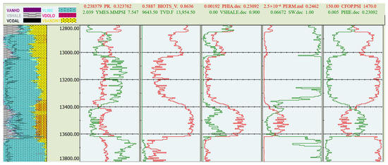
Figure 4.
Stratigraphic comprehensive parameter profile.

Table 1.
Pumping schedule.
Table 2.
Production parameters.
Parameter sensitivity analysis is a systematic method for evaluating how changes in model input parameters affect the model outputs. Its main goal is to pinpoint the most critical parameters for model outputs, thereby optimizing model structure, boosting model performance, cutting computational costs, and enhancing model interpretability and reliability. In this study, we conducted a local sensitivity analysis of the input parameters. This involves changing one parameter at a time while keeping the others constant and observing the model output changes, in line with the controlled variable method. The workflow involves automatically launching the GOHFER software via macro commands and batch-modifying input parameters across different ranges using Python. For each input parameter, 10 simulation scenarios with varied values are conducted. The effects of these parameter changes on fracture geometric morphology and production are recorded, aggregated, and visualized. This process ultimately generates variation curves illustrating how fracture geometry and production respond to different parameters.
This approach involves using macro commands to automatically launch the GOHFER software and employing Python to batch-modify input parameters across different ranges. For each set of input parameters, 10 simulations are conducted. The effects of these parameters on fracture geometry and production are observed, recorded, aggregated, and visualized to generate curves showing how fracture geometry and production vary with different parameters. Parameter sensitivity analysis can also uncover useful features in data, capturing all valuable information from the original dataset for model training. Given the numerous and intercoupled fracturing parameters, this analysis focuses on key factors affecting fracturing outcomes. These factors are summarized from engineering aspects like stage perforation, fracturing fluid, proppant, and pumping schedules, as well as geological aspects such as reservoir properties and rock mechanics, drawing on previous research on fracture propagation.
3.3. Neural-Network Model Training
The neural-network model for predicting fracture propagation is structured as follows: an artificial neural network is employed, and its accuracy is enhanced by adjusting parameters such as the activation function, optimizer, and number of neurons.
During the training phase, the model uses 16 input parameters that cover reservoir characteristics and fracturing operation data, with fracture geometric parameters as output parameters. The dataset is divided into training and testing sets in an 8:2 ratio to train the model. The neural network consists of two hidden layers with eight neurons each. The Tanh function is selected as the activation function, the learning rate is set at 0.001, and the Adam optimizer is used to further improve the model’s accuracy. Its neural network structure is shown in Figure 5.
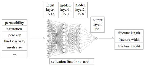
Figure 5.
Neural-network schematic diagram.
R2 reflects the model’s ability to explain data variability. It ranges from 0 to 1, and a value closer to 1 means the model has a better fit. The mean squared error (MSE) is the average of the squared differences between actual and predicted values. Since it squares the errors, it is sensitive to larger errors. A smaller MSE means the model has higher prediction accuracy. The root mean squared error (RMSE) has the same dimensions as the original data. It represents the standard deviation between the model’s predicted and actual values, with lower values indicating higher prediction accuracy. The explained-variance score (EVS) also ranges from 0 to 1. A value closer to 1 indicates a better model fit. The mean absolute error (MAE) is the average of the absolute differences between the actual and predicted values. It shows the average size of the model’s prediction errors. The smaller the MAE, the higher the prediction accuracy. Unlike the MSE, the MAE is less sensitive to outliers:
where is the true value, is the predicted value, is the average of the true values, is the variance of the residuals, and is the variance of the true values. In this study. , the , the , the , and the are used to evaluate model training outcomes. These metrics provide a comprehensive assessment of the model performance, thereby enhancing its credibility.
4. Results
4.1. Establishment of a Fracturing Big Dataset
This study combined Python code with macro commands to achieve automated batch processing of hydraulic-fracturing simulations, significantly enhancing simulation efficiency.
According to the research in this paper, when conducting 100 simulations, the manual method takes a total of 24 h, averaging 15 min per simulation, while the automated batch simulation takes only 4 h in total, averaging just 2 min per simulation. It is evident that automated batch simulation can significantly enhance the efficiency of fracture simulation. Moreover, as the number of simulations increases, this improvement in efficiency becomes even more pronounced. In addition to boosting efficiency, automated batch simulation can reduce operational complexity and minimize the risk of errors that may be caused by manual operations during repetitive tasks.
During automated batch simulations, a large volume of input and output parameters is generated. Based on empirical analysis, three key categories of input parameters were initially screened: reservoir data, including pressure coefficient, relative permeability coefficient, and water saturation, which reflect the fundamental physical properties of the reservoir and directly influence fracture propagation behavior; logging data, encompassing porosity, permeability, and saturation, which provide critical inputs for fracture simulation and enable more accurate predictions of fracture propagation and production; and fracturing operation data, involving fracturing fluid type, injection rate, and pressure conditions, which govern the kinetic processes of fracture propagation and are critical in controlling fracture geometry and distribution. To comprehensively evaluate fracture propagation outcomes, this study defined three categories of output parameters: fracture geometric parameters, including fracture length, width, and height, which directly relate to the effective contact areas and connectivity of fractures and serve as key indicators for evaluating fracture propagation quality; fracture conductivity, which represents the ability of fractures or channels to allow fluid passage and directly impacts well productivity and economic benefits, with higher conductivity facilitating smoother fluid flow into the wellbore and enhancing recovery rates; and production, which refers to daily or cumulative oil well production post-fracturing and serves as an economic metric to evaluate the ultimate effectiveness of fracturing operations. Through the design and screening of these input and output parameters, this study provides a scientific basis for automated batch processing of fracture simulations, significantly enhancing simulation efficiency and result reliability.
Based on the various input parameters in Table 3 and Table 4, automated batch simulations can be carried out. After simulation, a large number of fracture parameters are generated. Fracture length, width and height are taken as examples. Figure 6 shows the distribution of output parameters in this process. It can be seen that these parameters meet the characteristics of normal distribution, in line with actual field experience. Therefore, the big dataset we have established is qualified. The detailed input and output parameters are listed in the Table 3 and Table 4 below.
Table 3.
Input parameters.
Table 4.
Output parameters.
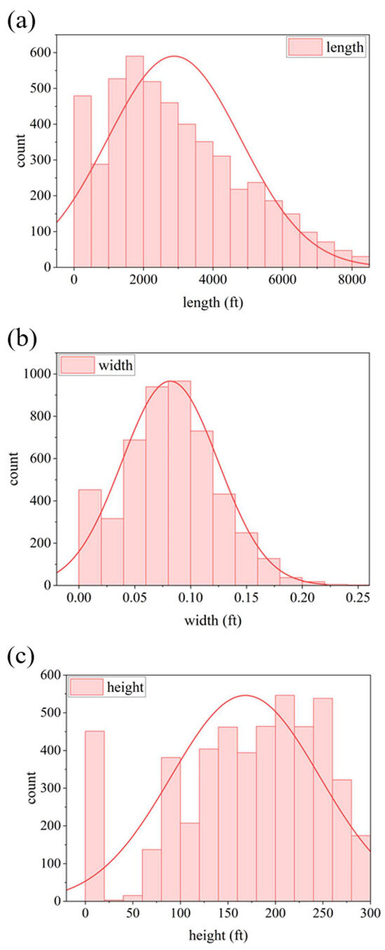
Figure 6.
Distribution of fracture parameters resulting from batch automatic simulation: (a) fracture length, (b) fracture width, and (c) fracture height.
4.2. Data Sensitivity Analysis Results
Through sensitivity analysis of hydraulic-fracturing operational parameters, this study investigated the response patterns of stimulated reservoir volume (SRV) to variations in construction parameters. The results revealed significant correlations between the SRV parameters and operational parameters. To further quantify these relationships, curve diagrams of influencing factors on fracture geometric morphology and box plots for correlation analysis of fracture geometric parameters were constructed.
As shown in Figure 7, this section investigates the sensitivity of fracture length to a variety of geological and operational parameters through systematic variation while holding all other conditions constant. The resulting trends are illustrated in Figure 7a–n.
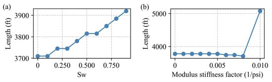
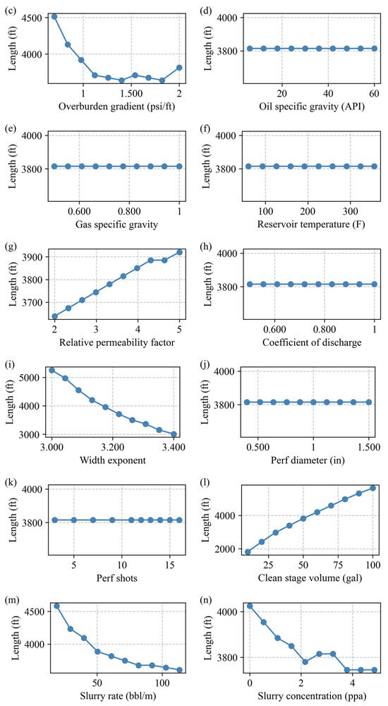
Figure 7.
Curve diagrams of influencing factors on fracture geometric morphology: (a) Sw, (b) modulus stiffness factor (1/psi), (c) overburden gradient (psi/ft), (d) oil-specific gravity (API), (e) gas-specific gravity, (f) reservoir temperature (F), (g) relative permeability factor, (h) coefficient of discharge, (i) width exponent, (j) perf diameter (in), (k) perf shots, (l) clean-stage volume (gal), (m) slurry rate (bbl/m), and (n) slurry concentration (ppa).
Fracture length is notably sensitive to fluid-related rock-weakening effects and formation compliance. As shown in Figure 7a,b,g, water saturation (Sw), the modulus stiffness factor (1/psi), and the relative permeability factor all exhibit positive correlations with fracture length. Increased Sw lowers effective stress and rock strength, facilitating fracture propagation. Similarly, higher formation compliance (lower stiffness) allows fractures to grow more easily under constant pressure input. Enhanced relative permeability promotes more efficient pressure transmission and fluid leakoff, further contributing to fracture extension.
Conversely, parameters representing in situ stress and pressure resistance exhibit strong negative impacts on fracture growth. Figure 7c highlights a pronounced inverse relationship between overburden gradient and fracture length: greater overburden stress restricts fracture development by increasing the minimum horizontal stress. Additionally, the width exponent (Figure 7i) negatively affects fracture length by promoting fracture width growth at the expense of length, particularly under constant injection volumes.
Operational fluid parameters further demonstrate varying impacts. Clean-stage volume (Figure 7l) shows a clear positive relationship with fracture length, affirming that higher fluid volumes supply the energy necessary for extended fracture growth. In contrast, Figure 7m,n show that higher slurry rates and proppant concentrations tend to reduce fracture length. Elevated slurry rates may increase fluid leakoff or reduce pressure sustainability, while excessive proppant concentrations increase the risk of early screenout, hindering fracture continuity.
Several parameters exhibit negligible influence on fracture length within the studied ranges. These include oil- and gas-specific gravity, reservoir temperature, the coefficient of discharge, perforation diameter, and shot density (Figure 7d–f,h,j,k). These factors may influence other aspects of well performance or initial fracture geometry but do not significantly impact fracture propagation under the given conditions.
Figure 8 uses a tornado diagram to show the influences of different geological parameters on hydraulic fractures. At the same time, the analysis identifies water saturation, rock stiffness, overburden gradient, relative permeability, clean-stage volume, slurry rate, and proppant concentration as primary drivers of fracture length variation. Grouping based on physical mechanisms highlights two dominant trends: rock and fluid properties that enhance stress transfer and reduce resistance promote longer fractures and elevated stress or operational inefficiencies that limit fracture growth. These insights are essential for optimizing fracture design and improving stimulation outcomes in unconventional reservoirs.
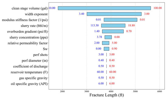
Figure 8.
Sensitivity of geometric morphology to fracture length. The blue number represents the minimum value of the parameter, and the red number represents the maximum value of the parameter.
As shown in Figure 9, this section investigates the sensitivity of fracture height and length to various operational parameters related to the fracturing process. The box plots in Figure 9a–f illustrate the influences of variables such as pumping rate, proppant mesh size, average proppant concentration, and stage length on fracture dimensions. This analysis focuses on isolating the impact of each parameter by holding other variables constant.
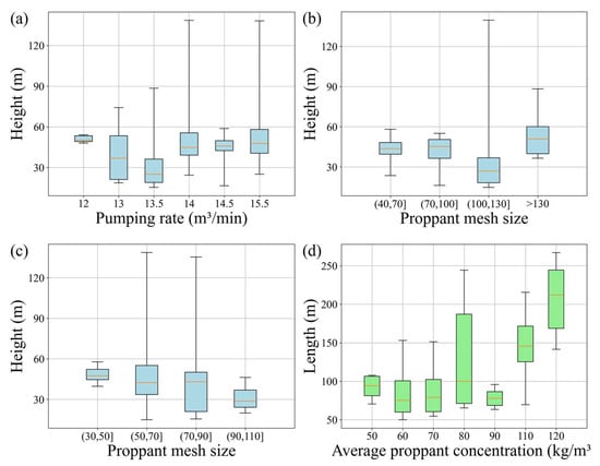
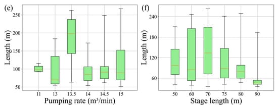
Figure 9.
Box plot for correlation analysis of fracture geometric parameters in hydraulic fracturing: (a) pumping rate (m3/min), (b,c) proppant mesh size, (d) average proppant concentration (kg/m3), and stage length (m). (e) pumping rate (m3/min), (f) stage length (m).
Figure 9a,e present the effect of the pumping rate on fracture height and length, respectively. Both figures reveal that increasing the pumping rate does not produce a consistent trend in fracture growth. Instead, the resulting fracture height and length exhibit substantial variability, especially at intermediate rates (e.g., 13.5 to 14.5 m3/min). This suggests that while a higher pumping rate may supply more energy for fracture propagation, it can also increase fluid leak-off and turbulence, introducing inconsistency in fracture development. The interaction between fluid dynamics and formation properties likely leads to these nonlinear and dispersed outcomes.
Figure 9b,c demonstrate the influence of proppant mesh size on fracture height. A general trend is observed in which extremely fine (>130) or coarse (30–50) proppant sizes tend to support greater fracture height. Finer proppants may better suspend in fluid and migrate further, while coarser proppants may help sustain wider fracture openings and resist closure. However, intermediate sizes exhibit more dispersion, suggesting a complex balance between transportability and propping efficiency.
Figure 9d highlights a clear positive relationship between average proppant concentration and fracture length. As the proppant concentration increases from 50 to 120 kg/m3, both the median and upper quartile of the fracture length expand substantially. This indicates that higher proppant concentrations improve fracture conductivity and structural integrity, enabling fractures to propagate further without premature closure or screenout. However, excessively high concentrations may still risk bridging or screenouts under certain flow conditions.
Figure 9f depicts the effect of stage length on fracture length. A decreasing trend is evident: longer stage lengths (80–90 m) correspond to significantly reduced fracture lengths compared to shorter stages (50–70 m). This may be due to the reduced energy concentration and pressure per unit interval in longer stages, resulting in less efficient fracture propagation. Shorter stages tend to concentrate energy more effectively, thus promoting more extensive fracture development.
Operational parameters such as pumping rate, proppant mesh size, proppant concentration, and stage length have varied effects on fracture dimensions. While proppant concentration and stage length show more consistent trends, pumping rate and mesh size introduce greater variability, emphasizing the need for careful optimization and calibration in field applications.
Through systematic parametric sensitivity analyses of both fracture length and height, this study identifies and categorizes key geological and pumping parameters influencing fracture propagation. The specific impact levels and impact causes are summarized in Table 5. Parameters such as water saturation, modulus stiffness, relative permeability, and clean-stage volume consistently exhibit a positive correlation with fracture extension, highlighting their role in facilitating pressure transmission and rock deformation. Conversely, factors such as overburden gradient, slurry rate, proppant concentration, and width exponent exert a constraining effect, either by increasing mechanical resistance or promoting inefficient fracture geometries. Variables including fluid properties (oil/gas-specific gravity, temperature) and perforation design (diameter, shot density) were found to have minimal impact under controlled conditions. These findings underscore the importance of fluid system design and stress environment in optimizing hydraulic-fracturing performance and provide a targeted basis for improving stimulation strategies in unconventional reservoirs.
Table 5.
Summary of sensitivity analysis on fracture geometry.
4.3. Surrogate-Model Establishment
This study generated 12,000 groups of fracture geometric-parameter data, constructing a big dataset for machine-learning training. To ensure data quality, raw data were preprocessed through cleaning and normalization to eliminate noise and standardize units. The processed data were used as inputs for the neural-network surrogate model designed to predict fracture geometry.
During model training, optimal hyperparameters were experimentally determined. Results indicated that the model achieved the best predictive performance when the learning rate was set to 0.0001 and the batch size was 32. To further optimize the model performance, adjustments were made to the number of hidden layers in the neural network. Experiments revealed that increasing the hidden layers to three did not significantly improve the accuracy but instead increased the model complexity, leading to reduced training efficiency and overfitting. Consequently, a two-layer hidden architecture was selected as the optimal balance between prediction efficiency and model performance. After determining the hyperparameters—two hidden layers with eight neurons each and the tanh activation function—we trained and predicted fracture length, width, and height separately. The results shown in Figure 10 demonstrate good predictive performance.
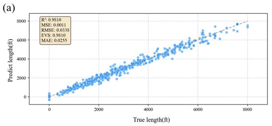
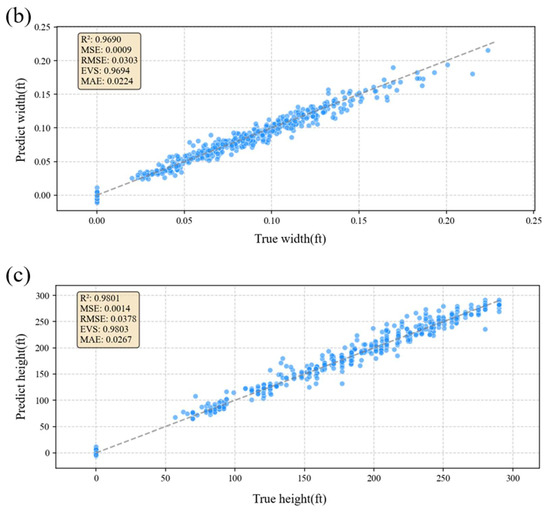
Figure 10.
Model prediction effects: (a) fracture length, (b) fracture width, and (c) fracture height. The horizontal axes of the figures represent the actual values of the parameters, and the vertical axes represent the model-predicted values. The upper left corner of the figure shows some evaluation indicators of the model.
The trained neural network demonstrated high predictive accuracy, with the training results compared in Figure 11. As shown in Figure 11, the model’s predicted values closely align with actual values, validating the effectiveness of the neural-network surrogate model.
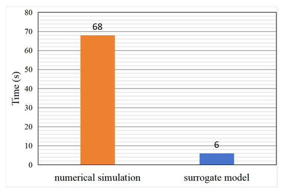
Figure 11.
Comparison of model efficiency. The orange bar represents the average time to predict fracture morphology using numerical simulation software. The blue bar on the right shows the time the surrogate model needs to predict 100 fracture morphology sets.
The surrogate model successfully established a dynamic link between the pumping process and fracture propagation. It can rapidly predict fracture geometric morphology and stimulated reservoir volume (SRV) changes based on real-time pumping curves. Currently, the model’s response time is less than 10 s, significantly enhancing real-time decision-making capabilities during fracturing operations. This achievement provides critical technical support for advancing the intelligence and efficiency of hydraulic fracturing.
5. Discussion
Traditional fracture prediction methods primarily rely on physics-based models and commercial numerical simulation software [44,45,46]. However, these approaches face several significant challenges. First, they are computationally intensive and lack the flexibility to adapt to real-time field conditions, limiting their effectiveness in guiding fracturing operations. Second, the time-consuming nature of numerical simulations makes them unsuitable for addressing small-sample problems often encountered in oilfield applications.
To address these limitations, this study introduces automated batch numerical simulation as a key innovation. This approach enables the large-scale and efficient generation of fracturing simulation data, laying a robust foundation for subsequent surrogate-model training and sensitivity analysis. Compared to traditional manual simulation workflows, the automated process substantially enhances parameter space coverage and accelerates the execution of simulation tasks, thereby supporting systematic exploration of multiple input variables. Moreover, automation ensures consistency and repeatability in the simulation process, effectively minimizing human errors and improving data quality and reliability. By leveraging this automated mechanism, a large-scale, structurally uniform training dataset can be rapidly constructed, significantly shortening the development cycle of data-driven models. When integrated with high-performance computing platforms, the workflow can be further scaled to accommodate a broader range of operating conditions and more complex application scenarios.
The surrogate model established in this paper is trained based on numerical simulation data and may not be able to fully capture the complexity of the real geological environment, such as reservoir heterogeneity, changes in fluid properties, and operational uncertainties. Model performance may degrade significantly under extreme conditions, including high-pressure/high-temperature settings, high proppant concentrations, or strongly anisotropic formations. Additionally, current models lack the capacity to detect and respond to fracture interactions and dynamically evolving boundary conditions during real-time fracturing, which may lead to deviations between predicted and actual results.
To enhance model robustness and field applicability, future research will focus on the following three directions:
- Integration of Physically Constrained Models: By incorporating physics-informed neural networks (PINNs), the training process can embed governing physical laws—such as fluid flow and stress equilibrium—thereby improving the model’s extrapolation capability, physical consistency, and generalization to unseen conditions.
- Real-Time Data Fusion and Dynamic Updating: Future models will incorporate real-time monitoring data, including microseismic fracture mapping, bottomhole pressure responses, and surface injection parameters. Establishing a closed-loop feedback mechanism will allow for dynamic parameter updating based on sensor feedback, enhancing real-time adaptability and prediction stability.
- Transfer Learning and Domain Adaptation: To bridge the gap between synthetic and real field data, transfer learning strategies will be employed. Pretraining on simulated datasets followed by fine-tuning with limited field data—such as diagnostic fracture injection tests (DFITs) or early production responses—can improve model adaptability across diverse geological settings while reducing data demands for deployment.
Collectively, these advancements are expected to significantly improve the robustness, predictive accuracy, and operational adaptability of the model. Ultimately, the integration of physical knowledge, real-time feedback, and adaptive learning will drive the development of intelligent, data-driven fracturing models that offer precise and efficient support for field-scale design optimization and decision-making.
6. Conclusions
This study integrates big-data technology and machine learning to monitor hydraulic-fracturing processes and predict post-fracturing fracture parameters, achieving the following key achievements:
A closed-loop workflow integrating Python scripts and macro commands was developed to automate fracturing simulations. This framework reduced simulation time by 83% (from 24 h to 4 h for 100 simulations) while minimizing human errors caused by manual parameter configuration. The workflow encompasses input preprocessing, parallel task execution, and automated post-processing, enabling the generation of a structured dataset containing 12,000 fracture geometry cases.
Through parameter sensitivity analysis, this study has pinpointed the key factors that influence fracture formation and development. Parameters such as effective porosity, water saturation, permeability, Young’s modulus, Poisson’s ratio, the relative permeability coefficient, the pressure coefficient, fracturing fluid density, fracturing fluid viscosity, proppant mesh size, proppant critical stress, proppant-specific gravity, time, cumulative sand volume, and injection rate have been identified as vital. These parameters have been chosen as crucial inputs for the neural-network model. Their selection not only enhances the model’s prediction accuracy but also offers insights into the model’s architecture. This allows for a more focused model-building process, improves the model’s interpretability, and makes it easier to fine-tune the model for better performance.
This study develops a deep-neural network-based surrogate model with two hidden layers of eight neurons each, trained using the Adam optimizer. It shows high predictive accuracy on both training and testing data. The model can predict fracture parameters and single-well production with high precision. It also identifies key pumping stages dynamically for real-time fracture propagation monitoring. With a response time of under 10 s, it continuously monitors fracture-stimulation–production-enhancement effects, offering solid technical support for optimizing fracturing parameters and evaluating production-enhancement outcomes.
Author Contributions
Conceptualization, X.H.; methodology, W.W.; writing—original draft, L.W.; validation, J.X.; formal analysis, C.L.; resources, L.C.; visualization, S.T.; supervision, Q.L.; investigation. All authors have read and agreed to the published version of the manuscript.
Funding
This work was supported by the PetroChina Xinjiang Oilfield Company (grant number XJYT-2024-JS-6398); National Natural Science Foundation of China (No. 52320105002, 52421002 and 52374017); Science Foundation of China University of Petroleum, Beijing (No. 2462025YJRC017); and National Key Laboratory of Petroleum Resources and Engineering (PRE/indep-1-2303).
Data Availability Statement
The data presented in this study are available on request from the corresponding author due to privacy restrictions from the company.
Acknowledgments
The authors gratefully acknowledge the technical and data support provided by PetroChina Xinjiang Oilfield Company. We also thank the anonymous reviewers for their valuable comments and suggestions, which have significantly improved the quality of this manuscript.
Conflicts of Interest
Authors Xiaodong He, Chang Li, and Lu Chen were employed by the Oil Production Technology Research Institute, Petrochina Xinjiang Oilfield Company. The remaining authors declare that this research was conducted in the absence of any commercial or financial relationships that could be construed as potential conflicts of interest.
References
- Wang, X.; Cai, B.; Li, S.; Ma, F.; Yan, Z.; Tong, Z.; Zhang, H. The history and outlook of reservoir stimulation technologies for oil and gas reservoirs in China. Oil Drill. Prod. Technol. 2023, 45, 67–75. (In Chinese) [Google Scholar] [CrossRef]
- Liao, Q.; Wang, B.; Chen, X.; Tan, P. Reservoir Stimulation for Unconventional Oil and Gas Resources: Recent Advances and Future Perspectives. Adv. Geo-Energy Res. 2024, 13, 7–9. [Google Scholar] [CrossRef]
- Wang, T.; Cheng, L.; Xiang, Y.; Cheng, N.; Wang, B.; Zhou, H. Numerical simulation of fracture-propagation behavior under gravel influence. Xinjiang Oil Gas 2023, 19, 42–48. (In Chinese) [Google Scholar] [CrossRef]
- Jiang, T.; Zhou, J.; Liao, L. Current status and development trends of intelligent fracturing technology worldwide. Pet. Drill. Tech. 2022, 50, 1–9. (In Chinese) [Google Scholar]
- Sprunger, C.; Muther, T.; Syed, F.I.; Dahaghi, A.K.; Neghabhan, S. State of the Art Progress in Hydraulic Fracture Modeling Using AI/ML Techniques. Model. Earth Syst. Environ. 2022, 8, 1–13. [Google Scholar] [CrossRef]
- Zheng, Y.; Wang, Y.; Liang, X.; Xue, Q.; Liang, E.; Wu, S.; An, S.; Yao, Y.; Liu, C.; Mei, J. A Deep Learning Approach for Signal Identification in the Fluid Injection Process during Hydraulic Fracturing Using Distributed Acoustic Sensing Data. Front. Earth Sci. 2022, 10, 999530. [Google Scholar] [CrossRef]
- Zhang, S.; Chen, Z. Application status and prospects of artificial intelligence in fracturing technology. Petro-Leum Drill. Tech. 2023, 51, 69–77. (In Chinese) [Google Scholar]
- Jia, J.; Fan, Q.; Jing, J.; Lei, K.; Wang, L. Intelligent Hydraulic Fracturing under Industry 4.0—A Survey and Future Directions. J. Pet. Explor. Prod. Technol. 2024, 14, 3161–3181. [Google Scholar] [CrossRef]
- Yadav, A.; Khanna, M.; Bhatia, G.; Nanda, D.; Gemini, P. Real-Time Decision Support in Optimizing Well Production and Hydraulic Fracturing Operations Using Digital Twins. In Proceedings of the EAGE Conference on Energy Excellence: Digital Twins and Predictive Analytics, Kuala Lumpur, Malaysia, 15–16 October 2024; European Association of Geoscientists & Engineers: Bunnik, The Netherlands, 2024; pp. 1–3. [Google Scholar]
- Liu, Y.-Y.; Ma, X.-H.; Zhang, X.-W.; Guo, W.; Kang, L.-X.; Yu, R.-Z.; Sun, Y.-P. A Deep-Learning-Based Prediction Method of the Estimated Ultimate Recovery (EUR) of Shale Gas Wells. Pet. Sci. 2021, 18, 1450–1464. [Google Scholar] [CrossRef]
- Qu, H.-Y.; Zhang, J.-L.; Zhou, F.-J.; Peng, Y.; Pan, Z.-J.; Wu, X.-Y. Evaluation of Hydraulic Fracturing of Horizontal Wells in Tight Reservoirs Based on the Deep Neural Network with Physical Constraints. Pet. Sci. 2023, 20, 1129–1141. [Google Scholar] [CrossRef]
- Xu, Z.; Lu, P. Current status of hydraulic-fracturing technology in China. Petrochem. Ind. Technol. 2017, 24, 280. (In Chinese) [Google Scholar]
- Hattori, G.; Trevelyan, J.; Augarde, C.E.; Coombs, W.M.; Aplin, A.C. Numerical Simulation of Fracking in Shale Rocks: Current State and Future Approaches. Arch Comput. Methods Eng. 2017, 24, 281–317. [Google Scholar] [CrossRef]
- Lecampion, B.; Bunger, A.; Zhang, X. Numerical Methods for Hydraulic Fracture Propagation: A Review of Recent Trends. J. Nat. Gas Sci. Eng. 2018, 49, 66–83. [Google Scholar] [CrossRef]
- Liu, X. Research and Application of Real-Time Monitoring and Interpretation Technology for Hydraulic Fracturing. Ph.D. Thesis, Southwest Petroleum University, Chengdu, China, 2005. (In Chinese). [Google Scholar]
- Yang, M. Research and Design of a Real-Time Tracking and Optimization Analysis System for Hydraulic Fracturing. Master’s Thesis, Southwest Petroleum University, Chengdu, China, 2019. (In Chinese). [Google Scholar]
- Alhemdi, A.; Gu, M. A Robust Workflow for Optimizing Drilling/Completion/Frac Design Using Machine Learning and Artificial Intelligence. In Proceedings of the SPE Annual Technical Conference and Exhibition, Houston, TX, USA, 3–5 October 2022; SPE: Houston, TX, USA, 2022; p. D021S022R002. [Google Scholar]
- Guo, J.; Ren, W.; Zeng, F.; Luo, Y.; Li, Y.; Du, X. Research progress and development prospects of intelligent optimization of fracturing parameters for unconventional oil and gas wells. Pet. Drill. Tech. 2023, 51, 1–7+179. (In Chinese) [Google Scholar]
- Sheng, M.; Tian, S.; Zhu, D.; Wang, T.; Liao, Q.; Li, G. Design concepts and pathways of an intelligent fractur-ing-pump-injection decision system. Nat. Gas Ind. 2024, 44, 108–113. (In Chinese) [Google Scholar]
- Tian, H.; Liu, R.; Li, D.; You, S.; Liao, Q.; Tian, S. Applications and Prospect of DeepSeek Large Language Model in Petroleum Engineering. Xinjiang Oil Gas 2025, 21, 55–63. (In Chinese) [Google Scholar] [CrossRef]
- Hou, L.; Zhang, F.; Elsworth, D. Post-Fracturing Evaluation of Fractures by Interpreting the Dynamic Matching Between Proppant Injection and Fracture Propagation. In Proceedings of the 57th U.S. Rock Mechanics/Geomechanics Symposium, Atlanta, Georgia, USA, 25–28 June 2023; ARMA: Alexandria, Australia, 2023. [Google Scholar]
- Qiao, J.; Gao, F.; Wu, D.; Tang, X. Combining Machine Learning and Physics Modelling to Determine the Natural Cave Property with Fracturing Curves. Comput. Geotech. 2023, 158, 105339. [Google Scholar] [CrossRef]
- Zhang, F.; Xu, M.; Deng, C.; Zhang, W.; Liu, C.; Rui, Z.; Emami-Meybodi, H. Deep-Learning Based LSTM for Production Data Analysis of Hydraulically Fractured Wells. In Proceedings of the International Petroleum Technology Conference, Dhahran, Saudi Arabia, 12–14 February 2024; p. D021S040R003. [Google Scholar]
- Zhang, P.; Gao, T.; Fu, J.; Li, R.; Zhang, E. Employing Neural Networks in Reservoir Simulation for Hydraulic-Fractured Unconventional Wells and a Case Study in STACK Area. In Proceedings of the SPE Oklahoma City Oil and Gas Symposium, Oklahoma City, OK, USA, 14–16 April 2025; SPE: Houston, TX, USA, 2025. [Google Scholar]
- Tosta, M.; Oliveira, G.P.; Wang, B.; Chen, Z.; Liao, Q. APyCE: A Python Module for Parsing and Visualizing 3D Reservoir Digital Twin Models. Adv. Geo-Energy Res. 2023, 8, 206–210. [Google Scholar] [CrossRef]
- Jiang, F.; Yang, S.; Cheng, Y.; Zhang, X.; Mao, Z.; Xu, F. Microseismic monitoring of rock bursts in coal mines. Chin. J. Geophys. 2006, 49, 1511–1516. (In Chinese) [Google Scholar]
- Zhang, X.; Tang, J.; Wei, Y.; Jia, C. Production-performance analysis and management of single wells in the Sulige gas field. J. Southwest Pet. Univ. (Sci. Technol. Ed.) 2009, 31, 110–114+187. (In Chinese) [Google Scholar]
- Li, D. Productivity-Prediction Study Based on Fracturing-Tracer Flowback Behavior. Master’s Thesis, China University of Petroleum (East China), Qingdao, China, 2024. (In Chinese). [Google Scholar]
- You, S.; Liao, Q.; Yue, Y.; Tian, S.; Li, G.; Patil, S. Enhancing Fracture Geometry Monitoring in Hydraulic Fracturing Using Radial Basis Functions and Distributed Acoustic Sensing. Adv. Geo-Energy Res. 2025, 16, 260–275. [Google Scholar] [CrossRef]
- Zimmer, U. Calculating Stimulated Reservoir Volume (SRV) with Consideration of Uncertainties in Microseismic-Event Locations. In Proceedings of the Canadian Unconventional Resources Conference, Calgary, AB, Canada, 15–17 November 2011; p. SPE-148610-MS. [Google Scholar]
- Suliman, B.; Meek, R.; Hull, R.; Bello, H.; Portis, D.; Richmond, P. Variable Stimulated Reservoir Volume (SRV) Simulation: Eagle Ford Shale Case Study. In Proceedings of the Unconventional Resources Technology Conference, The Woodlands, TX, USA, 12–14 August 2013; p. SPE-164546-MS. [Google Scholar]
- Ren, L.; Su, Y.; Zhan, S.; Hao, Y.; Meng, F.; Sheng, G. Modeling and Simulation of Complex Fracture Network Propagation with SRV Fracturing in Unconventional Shale Reservoirs. J. Nat. Gas Sci. Eng. 2016, 28, 132–141. [Google Scholar] [CrossRef]
- Assem, A.; Ibrahim, A.F.; Sinkey, M.; Johnston, T.; Marouf, S. A State-Of-The-Art Methodology in Live Measuring of Stimulated Reservoir Volume (SRV). In Proceedings of the SPE Argentina Exploration and Production of Unconventional Resources Symposium, Buenos Aires, Argentina, 20–22 March 2023; p. D021S008R002. [Google Scholar]
- Chen, Z.; Wei, Y.; Shi, L.; Hu, L.; Liao, X. A multi-mode fracture-network well-test model for fractured horizontal wells and parameter evaluation—A case study of the Jimsar shale-oil reservoir. Acta Pet. Sin. 2023, 44, 1706–1726. (In Chinese) [Google Scholar]
- Feng, Z.; Zhang, F.; Shen, X.; Yan, B.; Chen, Z. A Data-Driven Model for the Prediction of Stimulated Reservoir Volume (SRV) Evolution During Hydraulic Fracturing. In Proceedings of the 15th ISRM Congress, Salzburg, Austria, 9–14 October 2023; p. ISRM-15CONGRESS-2023-361. [Google Scholar]
- Zheng, W.; Su, W.; Tan, H. Analysis of influencing factors on fracturing performance of vertical and deviated wells in the central Sulige gas field. In Proceedings of the 2023 International Conference on Oil & Gas Field Exploration and Development, Wuhan, China, 20–22 September 2023; 2023; pp. 742–750. (In Chinese). [Google Scholar]
- Zheng, A.; Song, D.; Qin, Y.; Li, N.; Jia, Y.; Zhang, W. Quantitative evaluation of volume-fracturing effectiveness in con-glomerate reservoirs using trace chemical tracers. China Pet. Mach. 2024, 52, 95–103. (In Chinese) [Google Scholar] [CrossRef]
- Zhang, H. Study on the Evolution Mechanism of Dense-Cluster Volume-Fracturing Fracture Networks in Continental Shale-Oil Reservoirs. Ph.D. Thesis, Xi’an Shiyou University, Xi’an, China, 2024. (In Chinese). [Google Scholar]
- Ismail, A.; Azadbakht, S. A Comprehensive Review of Numerical Simulation Methods for Hydraulic Fracturing. Int. J. Numer. Anal. Methods Geomech. 2024, 48, 1433–1459. [Google Scholar] [CrossRef]
- Chen, M.; Guo, T.; Zou, Y.; Zhang, S.; Qu, Z. Numerical Simulation of Proppant Transport Coupled with Multi-Planar-3D Hydraulic Fracture Propagation for Multi-Cluster Fracturing. Rock Mech. Rock Eng. 2022, 55, 565–590. [Google Scholar] [CrossRef]
- Miskimins, J.L. Modeling of Hydraulic Fracture Height Containment in Laminated Sand and Shale Sequences. In Proceedings of the SPE Production and Operations Symposium, Oklahoma City, OK, USA, 23–25 March 2003. [Google Scholar]
- Ramurthy, M.; Towler, B.F.; Harris, H.G.; Barree, R.D. Effects of High Pressure-Dependent Leakoff (PDL) and High Pro-cess-Zone Stress (PZS) on Stimulation Treatments and Production. In Proceedings of the SPE Unconventional Resources Conference and Exhibition-Asia Pacific, Brisbane, Australia, 11–13 November 2013; p. SPE-167038-MS. [Google Scholar]
- McGowen, J.M.; Barree, R.D.; Conway, M.W. Incorporating Crossflow and Spurt-Loss Effects in Filtration Modeling Within a Fully 3D Fracture-Growth Simulator. In Proceedings of the SPE Annual Technical Conference and Exhibition, Houston, TX, USA, 3–6 October 1999; p. SPE-56597-MS. [Google Scholar]
- Valavanides, M.S.; Payatakes, A.C. Effects of Pore Network Characteristics on Steady-State Two-Phase Flow Based on a True-to-Mechanism Model (DeProF). In Proceedings of the Abu Dhabi International Petroleum Exhibition and Conference, Abu Dhabi, United Arab Emirates, 13–16 October 2002; p. SPE-78516-MS. [Google Scholar]
- Guiducci, C.; Collin, F.; Radu, J.P.; Pellegrino, A.; Charlier, R. Numerical Modeling of Hydro-Mechanical Fracture Behavior. In Proceedings of the ISRM 2003–Technology Roadmap for Rock Mechanics, Johannesburg, South Africa, 8–12 September 2003; p. ISRM-10CONGRESS-2003-073. [Google Scholar]
- Heng, Z.; Ersi, X.; Jie, L.; Jin, C. Study on the Fracture Propagation in Geothermal During the Hydraulic Fracturing Based on a Coupled Thermal-Hydraulic-Mechanical Modeling. In Proceedings of the 15th ISRM Congress, Salzburg, Austria, 9–14 October 2023; p. ISRM-15CONGRESS-2023-039. [Google Scholar]
Disclaimer/Publisher’s Note: The statements, opinions and data contained in all publications are solely those of the individual author(s) and contributor(s) and not of MDPI and/or the editor(s). MDPI and/or the editor(s) disclaim responsibility for any injury to people or property resulting from any ideas, methods, instructions or products referred to in the content. |
© 2025 by the authors. Licensee MDPI, Basel, Switzerland. This article is an open access article distributed under the terms and conditions of the Creative Commons Attribution (CC BY) license (https://creativecommons.org/licenses/by/4.0/).