Abstract
The integration of renewable energy resources (RES) into microgrids (MGs) poses significant challenges due to the intermittent nature of generation and the increasing complexity of multi-energy scheduling. To enhance operational flexibility and reliability, this paper proposes an intelligent energy management system (EMS) for MGs incorporating a hybrid hydrogen-battery energy storage system (HHB-ESS). The system model jointly considers the complementary characteristics of short-term and long-term storage technologies. Three conflicting objectives are defined: economic cost (EC), system response stability, and battery life loss (BLO). To address the challenges of multi-objective trade-offs and heterogeneous storage coordination, a novel deep-reinforcement-learning (DRL) algorithm, termed MOATD3, is developed based on a dynamic reward adjustment mechanism (DRAM). Simulation results under various operational scenarios demonstrate that the proposed method significantly outperforms baseline methods, achieving a maximum improvement of 31.4% in SRS and a reduction of 46.7% in BLO.
1. Introduction
Driven by the intensification of the global energy crisis and the escalating impacts of climate change, the demand for RES has surged worldwide. Among these, photovoltaic (PV) and wind power have emerged as critical components of the global energy mix, driving the transition toward sustainable development [1,2,3]. However, the intrinsic intermittency and unpredictability of RES present significant challenges to grid stability, energy consumption efficiency, and system reliability. To address these challenges, MGs have gained increasing attention due to their ability to integrate diverse RES and enable localized energy management. This has spurred the development of advanced EMS [4,5]. In EMS, the integration of efficient energy storage systems (ESS) and the design of adaptive energy dispatch strategies have become key approaches to improving the operational performance and reliability of MGs [2,6].
Energy storage technologies play a crucial role in addressing the intermittency and unpredictability of RES, ensuring that power generation and demand are matched in real time. The most common energy storage technologies include mechanical storage systems (MSS), BESS, supercapacitor (SC), and thermal storage systems (TSS), as well as compressed air energy storage (CAES) and HSS [7,8,9,10]. However, a single energy storage technology is often insufficient to meet both high energy density and long-duration storage requirements. As a solution, hybrid energy storage systems (HESS) were put forward, combining the advantages of multiple storage technologies. By integrating different types of storage, such as BESS for rapid response and CAES or HSS for long-term storage, HESS provides a more balanced solution that meets both short-term and long-term energy storage needs [9,10,11]. Li et al. [12] introduce a BESS and HHS as a cornerstone solution for establishing robust and sustainable MGs predominated by intermittent RES. This innovative configuration effectively minimizes economic expenditures while ensuring compliance with grid-connected power fluctuation mitigation requirements. Cui et al. [13] propose a multi-type EMS combining CAES and BESS, which functions within a multi-modal energy storage framework. This architecture demonstrates three core operational advantages: rapid-response capability, long-term energy balancing, and synergistic regulation modes with 91.8% round-trip efficiency. Guven et al. [14] propose a comprehensive optimization framework for battery-supercapacitor HESS (BESS/SC), addressing the critical challenge of enhancing energy storage efficiency in RES integration. Guezgouz et al. [15] proposed an integrated storage solution combining pumped hydro and battery systems, effectively overcoming the individual limitations of each technology and enhancing grid energy management efficiency through synergistic operation, with the result that the hybrid system achieves higher reliability at lower costs compared to single-storage technologies while reducing renewable generation curtailment.
In EMS, the effectiveness of the dispatch strategies plays a critical role in ensuring reliable operation, cost efficiency, and optimal use of RES. As MGs integrate more diverse and uncertain energy sources, scheduling becomes increasingly complex, requiring real-time decision-making and adaptability to fluctuating conditions [16]. Existing traditional scheduling methods primarily rely on mathematical programming [17], heuristic algorithms [18], and hybrid approaches [19]. Kassab et al. [20] proposed a joint multi-objective mixed-integer linear programming (MILP) algorithm to optimize both energy cost and emissions in an MG and improve local RES utilization. However, the method depends on accurate mathematical models and clearly defined physical information, which can be challenging to obtain for complex and dynamic systems, potentially limiting its applicability and accuracy. Xu et al. [21] investigated the energy scheduling problem in distributed generation systems and proposed a multi-strategy improved multi-objective particle swarm optimization algorithm (CMOPSO-MSI). This algorithm effectively enhances both economic performance and grid stability. However, traditional scheduling methods still face inherent limitations, such as a strong dependence on parameter tuning and difficulties in handling complex constraints.
DRL, as an emerging intelligent control method, combines the decision-making capability of RL with the feature representation power of DL. DRL enables agents to learn optimal policies through interaction with the environment without relying on explicit system models or handcrafted control rules [22,23]. In the context of EMS, DRL algorithms such as Proximal Policy Optimization (PPO), Deep Q-Networks (DQN), Deep Deterministic Policy Gradient (DDPG), and TD3 have been increasingly applied to tackle complex control and optimization problems [24]. Guo et al. [25] formulated the optimal energy management problem for MGs as an MDP framework that explicitly accounts for uncertainties in RES generation and load demand, and they employed the PPO method to derive optimal strategies. The numerical experiments conducted validate both the performance and computational advantages of their proposed approach. Alabdullah et al. [26] applied the DQN algorithm and modeled the energy management problem as a finite-horizon MDP. Without relying on an explicit MG model, the approach learns optimal strategies from historical data and system interaction. The final scheduling results show that the operation cost is within 2% of the theoretical optimum. Liang et al. [27] proposed an intelligent energy scheduling strategy based on the DDPG algorithm. Comparative analysis with conventional control methods reveals that the DDPG-based approach offers clear advantages in terms of cost-effectiveness, renewable energy utilization, and operational safety. Ruan et al. [28] conducted comparative experiments using both DDPG and TD3 algorithms against traditional methods such as PSO and mathematical programming under ideal input conditions. The results clearly demonstrate the adaptability of DRL approaches in terms of both optimization quality and computational efficiency.
Building upon the achievements of the above literature, a growing number of studies have adopted HESS and DRL algorithms for intelligent energy management. These efforts have demonstrated the potential of DRL in learning adaptive scheduling strategies and optimizing the operation of energy storage units in uncertain and dynamic environments. However, several critical challenges remain to be addressed. First, in EMS, the coordinated operation of multiple heterogeneous energy storage components is still difficult to achieve effectively due to differences in degradation behavior and operational constraints, among others. Second, as MG-EMS evolves, its scheduling objectives have become increasingly diverse, encompassing not only economic cost but also power stability, system responsiveness, and environmental indicators. For DRL-based methods, how to design and dynamically adjust the reward function to reflect multi-objective trade-offs has become a key technical bottleneck that directly affects policy convergence, stability, and real-world applicability.
Building upon the above discussion, to address the challenges of multi-storage coordination and multi-objective trade-offs in energy scheduling, an HHB-ESS is integrated into the MG framework. A novel algorithm, termed MOATD3 and based on DRAM, is proposed for the EMS of the MG. In the proposed model, three conflicting objectives are jointly optimized: (1) economic cost (EC); (2) system response stability (SRS); (3) battery life loss (BLO).
The proposed MOATD3 algorithm provides a flexible and adaptive decision-making framework that can dynamically adjust reward weights according to the system’s current state and optimization stage. By incorporating DRAM into the TD3 structure, the algorithm enhances the learning stability and adaptability of the policy, enabling efficient coordination between heterogeneous EMS and balancing multiple conflicting objectives in real time. The main contributions of this paper are summarized as follows:
- An HHB-ESS is integrated into the MG architecture to leverage the complementary characteristics of short-term and long-term energy storage technologies.
- Through comprehensive modeling of the MG system, three key performance indicators are formally defined to capture distinct aspects of system performance: EC, SRS, and BLO, thereby establishing a foundation for multi-objective optimization.
- Based on DRAM, a novel DRL algorithm named MOATD3 is proposed to address the multi-objective scheduling problem in the MG. The results demonstrate that the algorithm significantly improves performance in terms of economic efficiency, power exchange stability, and battery degradation suppression, validating its practical applicability and robustness.
The rest of this paper is structured as follows: Section 2 describes the architecture of the proposed microgrid system, including the mathematical models of its key components and the formulation of the multi-objective optimization problem. Section 3 introduces the MDP model and elaborates on the proposed MOATD3 algorithm, including its theoretical foundation and training procedure. Section 4 provides simulation results and performance analysis to validate the effectiveness of the proposed method. Section 5 concludes the paper and discusses future research directions.
2. Modeling of the MG Elements
Figure 1 illustrates a typical MG framework based on RES, as developed in this paper. As shown, the energy side of the MG comprises the main grid, along with two variable RES generation systems: PV and wind power. On the storage side, there is a controllable HSS and BESS. The HHS is composed of an electrolyzer, hydrogen tanks, and a fuel cell, while the BESS consists of n-batteries with different states and capacities. The load side represents electrical demand. The EMS unit serves as the control platform, which is primarily responsible for scheduling the HHB, coordinating the HESS, and managing energy transfer between the MG and the main grid. Its goal is to enhance the operational efficiency of the MG in terms of economic efficiency, power exchange stability, and battery degradation suppression. In the following sections, each component of the MG will be modeled in detail.
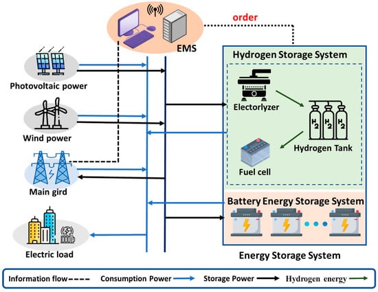
Figure 1.
Framework diagram of a hybrid MG.
2.1. RES Generation Modeling
The variable RES generation model describes the process of converting renewable energy into electrical energy, and, in this paper, it consists mainly of models for wind power and PV generation.
In the section on wind power generation, the energy harvested by the wind turbine depends on the wind speed and the inherent parameters of the turbine. Its mathematical model is given by the following equation [29]:
where represents the generated energy of the wind turbine at the time instant , and is the actual wind speed. is the turbine’s rated output power. , , and denote the turbine’s rated, cut-in, and cut-out wind speeds, respectively.
PV power generation technology utilizes solar energy to transform light into electrical energy, and its mathematical formulation is shown as follows [30]:
where represents the output power of the PV module at time , is the rated capacity of the PV module, is the derating coefficient of the PV module, is the solar radiation intensity at time , is the standard solar irradiance, is the temperature coefficient of the cell, is the cell temperature at time , and is the standard ambient temperature (typically 25 °C).
2.2. Battery Storage Charging and Discharging Power and Aging Modeling
The dynamic behavior of batteries is described through a mathematical charging and discharging power model. This model specifically characterizes the state transition process and operational constraints associated with BESS within the MG scheduling framework. Let represent the charge/discharge power of the battery at time , with positive values indicating discharging and negative values indicating charging. The state of charge (SoC), represented as , is updated according to the following formulation [31]:
where denotes the nominal capacity of battery , and represent the charge and discharge efficiencies, respectively, and is the control time step.
To ensure reliable and secure operation, the power and SoC of each battery are constrained by:
Due to the nonlinear aging characteristics of batteries, frequent charging and discharging behaviors can lead to SoC reduction and long-term capacity degradation. This degradation significantly impacts the reliability and operational efficiency of BESS. Therefore, it is essential to model both battery life loss and degradation cost to enable accurate system planning and economic dispatch. In this study, we adopt a modeling approach inspired by [32], which employs a linear approximation of the rainflow counting method to quantify cycle aging.
As shown in Figure 2, this method divides the full range of cycle depths into J segments (J = 4 is selected in this paper) and uses a piecewise linear function to model the relationship between cycle depth and battery cycle life loss , where . denotes the maximum capacity of the battery at time .
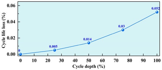
Figure 2.
Cycle life loss curve and 4-segment approximation.
Then, this method defines the marginal cost associated with each segment j:
where is the replacement cost associated with the battery .
The total degradation cost is calculated by aggregating the aging costs incurred at each time step based on the depth of charge and discharge power. The mathematical model is formulated as follows:
2.3. Hydrogen Energy Storage System Modeling
The HSS provides long-duration energy-balancing capabilities in the MG by enabling bidirectional conversion between electricity and hydrogen. The system allows surplus renewable electricity to be converted into hydrogen, stored over extended periods, and reconverted into electricity when needed. The following mathematical modeling process of the HSS is based on references [12,33,34].
The electrolyzer is used to convert surplus electricity from RES into hydrogen through water electrolysis. The amount of hydrogen generated by the electrolyzer at the time is given by:
where denotes the mass of hydrogen produced, is the input electrical power, is the electrolyzer efficiency, and is the lower heating value of hydrogen.
The electrolyzer operation may also be constrained by the rated power , such that:
The hydrogen tank temporarily stores the produced hydrogen for later use. Its storage level evolves according to the following state transition:
where is the hydrogen inventory, and are the charging and discharging efficiencies, respectively.
Since the hydrogen tank cannot simultaneously store and discharge hydrogen in practice, the model introduces a mutually exclusive operational constraint. The hydrogen flow is divided into the inflow and outflow , and a binary variable is used to indicate the operation mode at each time step. The constraints are expressed as:
where is the upper bound on the hydrogen tank’s operational flow rate.
Additionally, to ensure safe and reliable operation, the tank is subject to storage capacity limits:
The fuel cell performs the reverse conversion, transforming stored hydrogen into electrical energy. The corresponding hydrogen consumption is modeled as:
where is the electric power output, is the mass of hydrogen consumed by the fuel cell at time , and is the fuel cell efficiency. is further restricted by the maximum power output of the fuel cell:
2.4. Multi-Objective Optimization Modeling
To ensure reliable operation, the MG must satisfy power balance at each dispatch interval. That is, the total electrical demand from users and internal equipment must be met by available power sources, including RES generation, ESS, and the main grid. Mathematically, this can be expressed as:
where is the net power exchanged with the main grid (positive for import, negative for export), and is the total electrical load demand of the MG.
The scheduling optimization problem is designed to achieve the following three objectives:
- Obj 1: The system’s optimization cost includes the transaction cost , the degradation cost of the BESS, and the operation and maintenance costs and of both the BESS and HSS. The objective function is formulated as:where represents the electricity price at the time .
- Obj 2: To ensure the stable operation of the MG, it is necessary to minimize the fluctuation of power exchanged with the main grid. This objective is formulated as:where represents a reference value of the exchanged power, which can be set according to actual conditions.
- Obj 3: Battery degradation poses a significant challenge to the long-term performance and reliability of ESS. As degradation progresses, the battery’s usable SoC range shrinks, directly reducing the amount of energy available for flexible dispatch. Moreover, battery aging leads to increased replacement costs and, upon reaching end-of-life, may result in disposal and environmental concerns. Therefore, this paper incorporates BLO as a dedicated optimization objective:
3. Proposed MOATD3 Algorithm
In this chapter, the MG scheduling task is formulated as an MDP [34]. To address the challenges of multi-objective conflicts, environmental uncertainties, and the continuity of the action space encountered during microgrid operation, the MOATD3 algorithm is proposed to enable complex and efficient decision-making.
3.1. Modeling of MDP
DRL methods are typically based on the framework of MDP. The multi-energy MG dispatch strategies are formulated as an MDP, represented as the tuple , where:
State space : The state space includes all the observable information required to describe the current status of the microgrid system. The state vector at time step encapsulates the observable variables of the system, including:
Action space : The action space refers to the collection of all feasible control actions available to the agent. The action vector defines the power dispatch decisions for each controllable device:
Reward function : The reward function provides immediate feedback to the agent based on the current state and the action . The immediate reward of the MG is a dynamically weighted combination of three objectives:
where the weights are dynamically adjusted over time or based on system conditions to reflect the changing importance of each objective during scheduling. These weights satisfy the normalization condition: . , , and represent the normalized values of , , and at time , respectively.
Transition probability : The function characterizes the underlying system dynamics by defining the probability of reaching the next state after taking action in state .
is the discount factor.
3.2. Scheduling Method of the MOATD3 Algorithm
Figure 3 illustrates the architecture of MOATD3, showing how the agent engages with the environment. At each time step, the agent observes the current state of the environment, and based on this observation, it selects an action . The environment then returns the next state and a reward , which is dynamically adjusted by the DRAM. This mechanism allows the reward weights to adapt during training, helping the agent balance multiple objectives. The TD3 algorithm [34,35] adopts an actor–critic framework consisting of one actor network alongside two critic networks, which helps mitigate overvaluation bias in value estimation and stabilizes the training process. By combining the structural strengths of TD3 with the adaptive weighting strategy provided by DRAM, MOATD3 not only enhances learning stability but also effectively captures the balance between short- and long-term objectives, thus enabling more resilient and goal-aware policy learning in multi-objective environments.
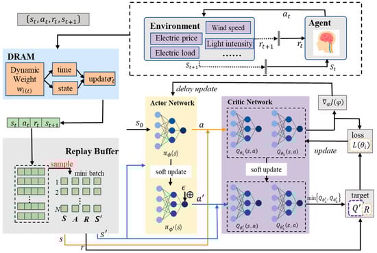
Figure 3.
The framework of the MOATD3 algorithm.
3.2.1. Theoretical Description
DRAM enables the agent to adjust the reward weights dynamically according to the current operational conditions of the MG, thereby enhancing adaptability and learning efficiency in complex, time-varying environments. In the model-free microgrid system, MOATD3’s DRAM adjusts multi-objective reward weights by increasing SRS during high load volatility to stabilize power and EC during peak prices to reduce grid purchases while encouraging low-price storage for adaptive objective balance. The weights are adjusted based on two main components:
Load volatility reflects short-term fluctuations in electricity demand. A high indicates instability, requiring greater focus on smoothing grid power exchange.
Cost gradient represents the relative rate of increase in operational cost. It guides the system to prioritize economic optimization when cost rapidly rises.
The specific formulas for are as follows:
where is the stability adjustment factor, a control parameter governing the influence strength of load fluctuations on weight updates and determining how sensitively weight transfer reacts to load changes; is the cost adjustment factor regulating the impact of electricity price fluctuations on weight updates and dictating the weight assigned to price changes in the allocation process.
This ensures that the reward weights automatically shift toward the most critical objective at each step, allowing the agent to dynamically balance between short-term economics and long-term sustainability.
RL provides a general paradigm for problems involving sequential decision-making, in which an agent engages with an environment modeled as an MDP. The objective of RL is to maximize the cumulative discounted reward, and the Bellman equation for the action–value function describes that the value of a state–action pair equals the immediate reward obtained by taking action in state , plus the expected discounted return from the next state under the policy :
Building upon this dynamic reward structure, the proposed MOATD3 algorithm extends the standard TD3 framework. TD3 maintains two independent critic networks , , and actor network . Instead of relying on a single critic to compute the Bellman target, TD3 uses the minimum value between the two critics when constructing the target value:
This clipped double Q-learning approach significantly reduces overestimation bias, ensuring that value targets remain conservative and improving the overall reliability of the critic’s evaluations.
TD3 introduces a target policy smoothing mechanism to tackle the issue of high sensitivity in policy updates. Specifically, when computing the target Q-value, a small amount of clipped Gaussian noise is added to the action output by the target actor network:
where represents Gaussian noise clipped within a specified range. This technique prevents the policy from exploiting narrow peaks in the estimated Q-function, promotes smoother value landscapes, and enhances the robustness of the learning process.
To improve training stability, TD3 adopts a delayed policy update strategy. The critic networks are updated at every time step by minimizing the mean squared error (MSE) between the predicted Q-value and the target value:
where N is the mini-batch size. The actor network is updated only once every d steps by maximizing the estimated Q-value from the first critic, using the deterministic policy gradient:
Finally, TD3 employs soft updates for the target networks to further improve training stability. After each update, the target networks are slowly updated towards the current networks:
where is the soft update coefficient.
Through the integration of clipped double Q-learning, target policy smoothing, delayed policy updates, and DRAM, MOATD3 achieves enhanced stability, improved adaptability to multiple objectives, and better long-term system optimization performance compared to conventional actor–critic algorithms.
3.2.2. Algorithm Workflow
The training of the MOATD3 algorithm is conducted over a maximum of N_episodes. Within each episode, the agent interacts with the environment for T = 24 consecutive time steps, corresponding to a full scheduling cycle over a 24 h horizon.
The MOATD3 training process starts by initializing the actor network , the critic networks , , and their corresponding target networks , , and . A replay buffer is also initialized for experience storage. At the beginning of each episode, the agent observes the initial state . At each time step t, an action is selected according to the policy with added Gaussian noise. After executing the action , the next state and the sub-rewards and are obtained. The dynamic reward weights are computed based on load volatility and cost gradient, and the total reward is constructed. The transition is stored in the replay buffer . A mini-batch N is randomly sampled from the replay buffer for network updates. The next action is generated with target policy smoothing as described in (24). The target Q-value is computed using the minimum of the two target critics following (23). The critic networks are updated by minimizing the loss function defined in (25). The actor network is updated with a delay for every d step by maximizing the critic output according to (26). Afterward, all target networks are softly updated following the soft update rule in (27). The above process is repeated iteratively across episodes until convergence.
This training cycle, including environment interaction, experience collection, network update, and target network adjustment, is repeated iteratively across all episodes until convergence. The training process of the proposed MOATD3 method is summarized in the pseudocode presented in Algorithm 1.
| Algorithm 1: Training process of the proposed MOATD3 method |
| 1: Initialize actor network and critic networks , with random parameters. 2: Initialize target networks: , and . 3: Initialize replay buffer . 4: for episode = 1 to N_episodes do: 5: Observe initial state from environment. 6: for t = 0 to T do: 7: Select action with exploration noise. 8: Project onto the feasible set defined by (4), (8), (11), (13) and (14). 9: Execute action , observe the next state , and sub-rewards: , . 10: Compute dynamic weights: . 11: Compute the total reward by (20). 12: Store transition into buffer . 13: Sample mini-batch of N transitions from . 14: Compute the target Q-value with target policy smoothing by (23). 15: Update critics by minimizing MSE loss: 16: Delayed actor update: 17: If t mod d then 18: Update the actor network: . 19: Update target networks by (27). 20: end if 21: 22: end for 23: end for |
4. Simulation Results
In this section, two different weather conditions are selected as representative scenarios, using 24 h data with a 1-hour time step for energy scheduling. To comprehensively assess the performance of the HHB-ESS and MOATD3 algorithm, comparative experiments are conducted under four different scenarios and strategies. The results demonstrate the proposed method’s advantages in handling dynamic energy demand and ensuring system stability.
4.1. Simulation Setup
To validate the performance of HHBESS-MOATD3, we construct a simulation framework based on a hybrid MG composed of wind power, PV systems, BESS, and HHB-ESS. RES generation and residential load demand under good and bad weather conditions are illustrated in Figure 4, capturing daily variation patterns essential for evaluating the robustness of the control strategy [34,36,37]. The cost functions of HHBESS-TD3 and HHBESS-DDPG are identical and the same as that of MOATD3. For the existing algorithms, the weight parameters = 0.5, = 0.3 and = 0.2 of the reward function are constants and remain unchanged throughout the entire scheduling process.
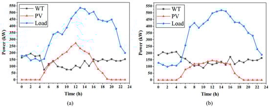
Figure 4.
RES and load demands data: (a) good weather; (b) bad weather.
The technical specifications of all system components, including PV and WT units and storage systems, are shown in Table 1. The parameters are selected based on practical system references [13,34,38,39] to ensure realism. A time-varying electricity pricing structure, as detailed in Table 2, is adopted to emulate realistic market-based incentives and guide optimal scheduling.

Table 1.
Parameters of each component in the hybrid MG.
Table 2.
Time-of-use electricity pricing.
As shown in Table 3, the proposed method is compared with three alternative scenarios. Scenario 1 replaces the hybrid energy storage system with a standalone BESS to assess the impact of storage configuration. Scenario 2 retains the HHB-ESS setup but substitutes the algorithm with TD3 to evaluate the improvement introduced by MOATD3. Scenario 3 combines HHB-ESS with DDPG as a benchmark. These four settings are designed to analyze the respective contributions of storage system structure and scheduling algorithm optimization to overall system performance.
Table 3.
Four scenario settings in the simulation experiments.
4.2. The Scheduling Results
This section demonstrates the training performance of the MOATD3 algorithm under the HHB-ESS configuration. As shown in Figure 5, the training reward curves span 120,000 time steps in both good weather and adverse weather scenarios. To facilitate observation of the reward variation process, some steps during the random sampling phases and after training convergence are excluded from the figure. The figure simultaneously displays both the raw rewards and the smoothed rewards.

Figure 5.
Training reward curve of the MOATD3 algorithm: (a) good weather; (b) bad weather.
The experimental results of the HHBESS-MOATD3 algorithm demonstrate its effectiveness in managing energy supply and demand within microgrids under different weather conditions. The algorithm was tested in two scenarios: good weather and adverse weather. Figure 6 illustrates the energy scheduling in both cases, including PV, wind, BESS, HSS (via electrolyzers and fuel cells), and interactions with the grid. In the bar chart, the region between the load curve and the x-axis (below the load curve) represents the power sources for the current load, while the negative values in the chart denote the electricity stored in the BESS and HESS by PV and WT. Meanwhile, the part where positive values in the bar chart exceed the load can offset the negative values, representing power balance.
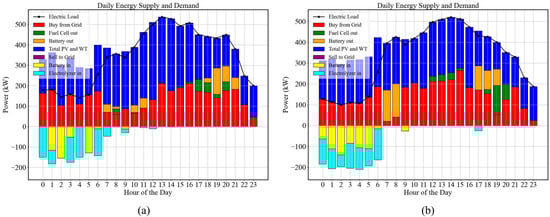
Figure 6.
HHBESS-MOATD3 scheduling results: (a) good weather; (b) bad weather.
The results indicate that HHBESS-MOATD3 (based on TD3) minimizes fluctuations in grid-purchased power at each time point through BESS/HSS scheduling, thereby stabilizing bidirectional power flow with the main grid. Under good weather conditions, the system benefits from higher renewable energy generation, primarily from PV and wind power, to maximize the self-utilization rate of self-generated power and minimize grid power procurement. By contrast, under adverse weather conditions, reduced PV and wind power generation lead to a significant increase in grid power purchases to meet load demand. At this point, the algorithm activates the battery and hydrogen energy storage systems more frequently through scheduling to ensure power supply stability and cost balance.
Additionally, Figure 7 further demonstrates the adaptability of the MOATD3 algorithm by showing the dynamic adjustment of the stability reward weight () and economic reward weight () over a 24 h cycle. Overall, the economic reward weight is higher during midday and evening peak electricity consumption periods due to higher electricity prices. Under good weather conditions, the high output and large intra-hour fluctuations of renewable energy make it prone to disrupting the main grid stability. Thus, the stability weight is generally higher. In adverse weather conditions, the system shifts its focus to the economy to maintain lower costs. This dynamic adaptation mechanism embodies the core advantage of the MOATD3 algorithm: intelligently balancing economic optimization and system stability based on real-time environmental changes.
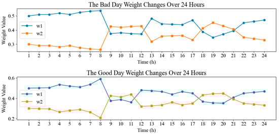
Figure 7.
The dynamic adjustment of reward weights in EMS optimization.
4.3. Comparative Experiment Analysis
This section presents a comparative analysis of the proposed HHBESS-MOATD3 method with other methods, including BESS-MOATD3, HHBESS-TD3, and HHBESS-DDPG. The comparative experiments are conducted under two scenarios: good weather and bad weather conditions. The dispatching strategies for ESS in six different scenarios are shown in Figure 8 and Figure 9. The performance of each method is evaluated based on three key metrics: EC, SRS, and BLO, which is shown in Table 4 with specific numerical values.
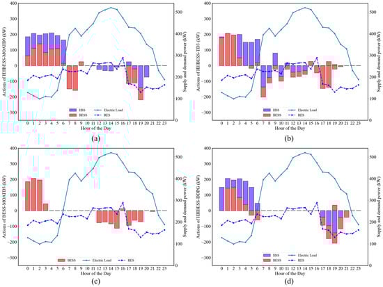
Figure 8.
Decision-making under good weather conditions using different methods: (a) HHBESS-MOATD3; (b) HHBESS-TD3; (c) BESS-MOATD3; (d) HHBESS-DDPG.
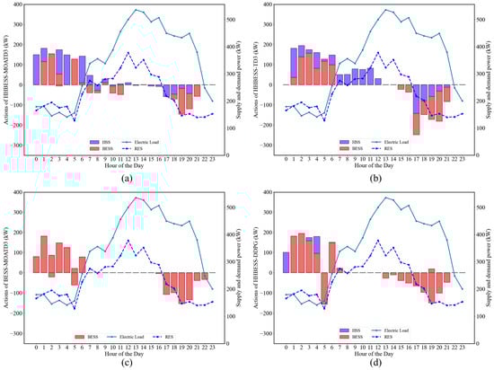
Figure 9.
Decision-making under bad weather conditions using different methods: (a) HHBESS-MOATD3; (b) HHBESS-TD3; (c) BESS-MOATD3; (d) HHBESS-DDPG.
Table 4.
Comparative results under different scenarios.
Model Analysis: Compared with the traditional BESS, integrating the HSS into the MG significantly enhances system performance. As shown in Table 4, the inclusion of HSS improves system flexibility, and HHBESS-MOATD3 achieves lower EC compared to the pure BESS configuration, particularly under bad weather conditions, where EC is reduced by approximately 8.0%. This indicates that the HSS configuration effectively utilizes the fast-response capability of batteries and the long-duration energy storage capacity of hydrogen systems, thereby reducing operational costs. In terms of stability, HHB-ESS improves grid stability by 17.2% and 30.3% under different weather conditions. Additionally, HHBESS-MOATD3 demonstrates significant improvements in power stability and battery life compared to BESS-MOATD3, with maximum improvements of 31.4% and 30.4%, respectively. This trade-off between short-term battery utilization and long-term hydrogen system activation is validated by an 8.0% lower EC of HHBESS-MOATD3 under bad weather, proving that hybrid storage balances immediate cost-saving with asset longevity.
Algorithm Comparison: Among the three algorithms, MOATD3 exhibits significant advantages over TD3 and DDPG. The Dynamic Reward Allocation Mechanism (DRAM) in MOATD3 increases the weight for stability when power fluctuations are large and increases the weight for economy when power purchase prices are high, enabling better trade-offs between economic efficiency and power stability. For example, compared with TD3, the MOATD3 algorithm reduces the SRS by 20.0% under good weather conditions and approximately 13.9% under bad weather conditions, with slightly lower costs than TD3. Similar effects are observed when compared with DDPG, indicating that MOATD3 can better adapt to changes in energy demand and environmental conditions by dynamically adjusting reward weights. Furthermore, thanks to the restriction on power purchase by economic weight during peak power consumption periods, the BLO achieved by HHBESS-MOATD3 is significantly lower than that of other algorithms, particularly optimized by 46.7% under good weather conditions. This result reflects the ability of the MOATD3 algorithm to balance the discharge of batteries and hydrogen energy storage, thereby minimizing battery degradation.
Overall, the comparative analysis highlights that the integration of HSS with BESS, combined with the adaptive nature of MOATD3, results in superior performance in terms of cost efficiency, power stability, and battery longevity. The HHBESS-MOATD3 method not only addresses the economic challenges of energy management but also significantly mitigates grid instability caused by renewable energy fluctuations, making it a more reliable solution for MG scheduling. The deep synergy between the DRAM and the TD3 architecture significantly enhances the model’s comprehensive performance in multi-objective energy management scenarios through a dual approach of adaptive target weight allocation and reinforcement learning process optimization.
Overall, the comparative analysis highlights that the integration of HSS with BESS, combined with the adaptive nature of MOATD3, results in superior performance in terms of cost efficiency, power stability, and battery longevity. The HHBESS-MOATD3 method not only addresses the economic challenges of energy management but also significantly mitigates grid instability caused by renewable energy fluctuations, making it a more reliable solution for MG scheduling.
5. Conclusions
This study develops an innovative microgrid EMS by integrating the HHB-ESS with the MOATD3 algorithm, addressing dynamic energy demand and multi-objective optimization challenges. A typical microgrid model and multi-objective optimization framework target economic operation includes EC, SRS, and BLO. Eight comparative simulations under two weather conditions validate the HHB-ESS/MOATD3 approach. The MOATD3 algorithm, using dynamic reward adjustment, outperforms traditional DRL methods (TD3/DDPG) in policy adaptability and robustness, balancing economic, stability, and battery life objectives effectively. Future work will focus on integrating diverse energy storage technologies, improving algorithm adaptability, validating large-scale/real MGs, and combining model-driven with data-driven methods to enhance scheduling reliability.
At the data validation level, systematic verification will be conducted based on more diverse weather datasets in the future, aiming to comprehensively cover the complex and changeable weather conditions in real-world scenarios. In terms of practical applicability, future work will focus on extending the algorithm validation to real microgrid datasets and conducting field tests in actual microgrid systems. This will involve integrating more diverse renewable energy profiles, complex load patterns, and real-time grid interaction constraints to ensure the robustness of the proposed framework in heterogeneous operational environments.
Author Contributions
Conceptualization, J.J. and D.A.; methodology, Y.Z.; software, J.J.; validation, Y.Z., J.J. and D.A.; formal analysis, J.J.; investigation, Y.Z.; resources, D.A.; data curation, J.J.; writing—original draft preparation, Y.Z.; writing—review and editing, J.J.; visualization, Y.Z.; supervision, D.A.; project administration, D.A.; funding acquisition, D.A. All authors have read and agreed to the published version of the manuscript.
Funding
This work was supported by the National Key R&D Program of China (No. 2024YFB4206500), and the National Natural Science Foundation of China (No. 62173268).
Data Availability Statement
No new data were created or analyzed in this study and all the data have been well presented in the manuscript.
Conflicts of Interest
The authors declare no conflict of interest.
References
- Olabi, A.G.; Abdelkareem, M.A. Renewable energy and climate change. Renew. Sustain. Energy Rev. 2022, 158, 112111. [Google Scholar] [CrossRef]
- Sayed, E.T.; Olabi, A.G.; Alami, A.H.; Radwan, A.; Mdallal, A.; Rezk, A.; Abdelkareem, M.A. Renewable energy and energy storage systems. Energies 2023, 16, 1415. [Google Scholar] [CrossRef]
- Sayfutdinov, T.; Patsios, C.; Greenwood, D.; Peker, M.; Sarantakos, I. Optimization-based modelling and game-theoretic framework for techno-economic analysis of demand-side flexibility: A real case study. Appl. Energy 2022, 321, 119370. [Google Scholar] [CrossRef]
- Saeed, M.H.; Fangzong, W.; Kalwar, B.A.; Iqbal, S. A review on microgrids’ challenges & perspectives. IEEE Access 2021, 9, 166502–166517. [Google Scholar]
- Gayen, D.; Chatterjee, R.; Roy, S. A review on environmental impacts of renewable energy for sustainable development. Int. J. Environ. Sci. Technol. 2024, 21, 5285–5310. [Google Scholar] [CrossRef]
- Thirunavukkarasu, G.S.; Seyedmahmoudian, M.; Jamei, E.; Horan, B.; Mekhilef, S.; Stojcevski, A. Role of optimization techniques in microgrid energy management systems—A review. Energy Strategy Rev. 2022, 43, 100899. [Google Scholar] [CrossRef]
- Mahmoud, M.; Ramadan, M.; Olabi, A.G.; Pullen, K.; Naher, S. A review of mechanical energy storage systems combined with wind and solar applications. Energy Convers. Manag. 2024, 210, 112670. [Google Scholar] [CrossRef]
- Rouholamini, M.; Wang, C.; Nehrir, H.; Hu, X.; Hu, Z.; Aki, H.; Zhao, B.; Miao, Z.; Strunz, K. A review of modeling, management, and applications of grid-connected Li-ion battery storage systems. IEEE Trans. Smart Grid 2022, 13, 4505–4524. [Google Scholar] [CrossRef]
- Boretti, A.; Castelletto, S. Hydrogen energy storage requirements for solar and wind energy production to account for long-term variability. Renew. Energy 2024, 221, 119797. [Google Scholar] [CrossRef]
- Zou, Y.; Tang, S.; Guo, S.; Wu, J.; Zhao, W. Energy storage/power/heating production using compressed air energy storage integrated with solid oxide fuel cell. J. Energy Storage 2024, 83, 110718. [Google Scholar] [CrossRef]
- Schubert, C.; Hassen, W.F.; Poisl, B.; Seitz, S.; Schubert, J.; Oyarbide Usabiaga, E.; Gaudo, P.M.; Pettinger, K.H. Hybrid energy storage systems based on redox-flow batteries: Recent developments, challenges, and future perspectives. Batteries 2023, 9, 211. [Google Scholar] [CrossRef]
- Li, S.; Zhu, J.; Dong, H.; Zhu, H.; Fan, J. A novel rolling optimization strategy considering grid-connected power fluctuations smoothing for renewable energy microgrids. Appl. Energy 2022, 309, 118441. [Google Scholar] [CrossRef]
- Cui, F.; An, D.; Xi, H. Integrated energy hub dispatch with a multi-mode CAES–BESS hybrid system: An option-based hierarchical reinforcement learning approach. Appl. Energy 2024, 374, 123950. [Google Scholar] [CrossRef]
- Guven, A.F.; Abdelaziz, A.Y.; Samy, M.M.; Barakat, S. Optimizing energy Dynamics: A comprehensive analysis of hybrid energy storage systems integrating battery banks and supercapacitors. Energy Convers. Manag. 2024, 312, 118560. [Google Scholar] [CrossRef]
- Guezgouz, M.; Jurasz, J.; Bekkouche, B.; Ma, T.; Javed, M.S.; Kies, A. Optimal hybrid pumped hydro-battery storage scheme for off-grid renewable energy systems. Energy Convers. Manag. 2019, 199, 112046. [Google Scholar] [CrossRef]
- Nawaz, A.; Zhou, M.; Wu, J.; Long, C. A comprehensive review on energy management, demand response, and coordination schemes utilization in multi-microgrids network. Appl. Energy 2022, 323, 119596. [Google Scholar] [CrossRef]
- Lu, S.; Wang, C.; Fan, Y.; Lin, B. Robustness of building energy optimization with uncertainties using deterministic and stochastic methods: Analysis of two forms. Build. Environ. 2021, 205, 108185. [Google Scholar] [CrossRef]
- Kim, H.J.; Kim, M.K. A novel deep learning-based forecasting model optimized by heuristic algorithm for energy management of microgrid. Appl. Energy 2023, 332, 120525. [Google Scholar] [CrossRef]
- Dinh, H.T.; Lee, K.H.; Kim, D. A Supervised-Learning based Hour-Ahead Demand Response of a Behavior-based HEMS approximating MILP Optimization. arXiv 2021, arXiv:2111.01978. [Google Scholar]
- Kassab, F.A.; Celik, B.; Locment, F.; Sechilariu, M.; Liaquat, S.; Hansen, T.M. Optimal sizing and energy management of a microgrid: A joint MILP approach for minimization of energy cost and carbon emission. Renew. Energy 2024, 224, 120186. [Google Scholar] [CrossRef]
- Xu, X.F.; Wang, K.; Ma, W.H.; Wu, C.L.; Huang, X.R.; Ma, Z.X.; Li, Z.H. Multi-objective particle swarm optimization algorithm based on multi-strategy improvement for hybrid energy storage optimization configuration. Renew. Energy 2024, 223, 120086. [Google Scholar] [CrossRef]
- Luo, D. Optimizing Load Scheduling in Power Grids Using Reinforcement Learning and Markov Decision Processes. arXiv 2024, arXiv:2410.17696. [Google Scholar]
- Matsuo, Y.; LeCun, Y.; Sahani, M.; Precup, D.; Silver, D.; Sugiyama, M.; Uchibe, E.; Morimoto, J. Deep learning, reinforcement learning, and world models. Neural Netw. 2022, 152, 267–275. [Google Scholar] [CrossRef]
- Yu, L.; Qin, S.; Zhang, M.; Shen, C.; Jiang, T.; Guan, X. A review of deep reinforcement learning for smart building energy management. IEEE Internet Things J. 2021, 8, 12046–12063. [Google Scholar] [CrossRef]
- Guo, C.; Wang, X.; Zheng, Y.; Zhang, F. Real-time optimal energy management of microgrid with uncertainties based on deep reinforcement learning. Energy 2022, 238, 121873. [Google Scholar] [CrossRef]
- Alabdullah, M.H.; Abido, M.A. Microgrid energy management using deep Q-network reinforcement learning. Alex. Eng. J. 2022, 61, 9069–9078. [Google Scholar] [CrossRef]
- Liang, T.; Chai, L.; Cao, X.; Tan, J.; Jing, Y.; Lv, L. Real-time optimization of large-scale hydrogen production systems using off-grid renewable energy: Scheduling strategy based on deep reinforcement learning. Renew. Energy 2024, 224, 120177. [Google Scholar] [CrossRef]
- Ruan, Y.; Liang, Z.; Qian, F.; Meng, H.; Gao, Y. Operation strategy optimization of combined cooling, heating, and power systems with energy storage and renewable energy based on deep reinforcement learning. J. Build. Eng. 2023, 65, 105682. [Google Scholar] [CrossRef]
- Jahannoosh, M.; Nowdeh, S.A.; Naderipour, A.; Kamyab, H.; Davoudkhani, I.F.; Klemeš, J.J. New hybrid meta-heuristic algorithm for reliable and cost-effective designing of photovoltaic/wind/fuel cell energy system considering load interruption probability. J. Clean. Prod. 2021, 278, 123406. [Google Scholar] [CrossRef]
- Hossain, M.A.; Pota, H.R.; Squartini, S.; Abdou, A.F. Modified PSO algorithm for real-time energy management in grid-connected microgrids. Renew. Energy 2019, 136, 746–757. [Google Scholar] [CrossRef]
- Harsh, P.; Das, D. Energy management in microgrid using incentive-based demand response and reconfigured network considering uncertainties in renewable energy sources. Sustain. Energy Technol. Assess. 2021, 46, 101225. [Google Scholar] [CrossRef]
- Xu, B.; Zhao, J.; Zheng, T.; Litvinov, E.; Kirschen, D.S. Factoring the cycle aging cost of batteries participating in electricity markets. IEEE Trans. Power Syst. 2018, 33, 2248–2259. [Google Scholar] [CrossRef]
- Irham, A.; Roslan, M.F.; Jern, K.P.; Hannan, M.A.; Mahlia, T.I. Hydrogen energy storage integrated grid: A bibliometric analysis for sustainable energy production. Int. J. Hydrogen Energy 2024, 63, 1044–1087. [Google Scholar] [CrossRef]
- Yousri, D.; Farag, H.E.; Zeineldin, H.; El-Saadany, E.F. Integrated model for optimal energy management and demand response of microgrids considering hybrid hydrogen-battery storage systems. Energy Convers. Manag. 2023, 280, 116809. [Google Scholar] [CrossRef]
- Fujimoto, S.; Hoof, H.; Meger, D. Addressing function approximation error in actor-critic methods. In Proceedings of the 35th International Conference on Machine Learning, Stockholm, Sweden, 10–15 July 2018; pp. 1587–1596. [Google Scholar]
- Sun, B.; Song, M.; Li, A.; Zou, N.; Pan, P.; Lu, X.; Yang, Q.; Zhang, H.; Kong, X. Multi-objective solution of optimal power flow based on TD3 deep reinforcement learning algorithm. Sustain. Energy Grids Netw. 2023, 34, 101054. [Google Scholar] [CrossRef]
- Saleem, M.I.; Saha, S.; Izhar, U.; Ang, L. Optimized energy management of a solar battery microgrid: An economic approach towards voltage stability. J. Energy Storage 2024, 90, 111876. [Google Scholar] [CrossRef]
- Silani, A.; Yazdanpanah, M.J. Distributed optimal microgrid energy management with considering stochastic load. IEEE Trans. Sustain. Energy 2018, 10, 729–737. [Google Scholar] [CrossRef]
- Li, J.; Xiao, Y.; Lu, S. Optimal configuration of multi microgrid electric hydrogen hybrid energy storage capacity based on distributed robustness. J. Energy Storage 2024, 76, 109762. [Google Scholar] [CrossRef]
Disclaimer/Publisher’s Note: The statements, opinions and data contained in all publications are solely those of the individual author(s) and contributor(s) and not of MDPI and/or the editor(s). MDPI and/or the editor(s) disclaim responsibility for any injury to people or property resulting from any ideas, methods, instructions or products referred to in the content. |
© 2025 by the authors. Licensee MDPI, Basel, Switzerland. This article is an open access article distributed under the terms and conditions of the Creative Commons Attribution (CC BY) license (https://creativecommons.org/licenses/by/4.0/).