Article

An Integrated Synthesis Approach for Emergency Logistics System Optimization of Hazardous Chemical Industrial Parks

1
School of Chemical Engineering, Dalian University of Technology, Dalian 116024, China
2
China Academy of Safety Science and Technology, Beijing 100012, China
3
Key Laboratory of Major Hazard and Chemical Industry Park System Safety, Ministry of Emergency Management, Beijing 100012, China
*
Authors to whom correspondence should be addressed.
Processes 2025, 13(8), 2513; https://doi.org/10.3390/pr13082513 (registering DOI)
Submission received: 11 July 2025 / Revised: 3 August 2025 / Accepted: 7 August 2025 / Published: 9 August 2025
(This article belongs to the Section Chemical Processes and Systems)

Abstract

The rapid clustering of Chemical Industrial Parks (CIPs) has escalated the risk of cascading disasters (e.g., toxic leaks and explosions), underscoring the need for resilient emergency logistics systems. However, traditional two-stage optimization models often yield suboptimal outcomes due to decoupled facility location and routing decisions. To address this issue, we propose a unified mixed-integer nonlinear programming (MINLP) model that integrates site selection and routing decisions in a single framework. The model accounts for multi-source supply allocation, enforces minimum safety distance constraints, and incorporates heterogeneous economic factors (e.g., regional land costs) to ensure risk-aware, cost-efficient planning. Two deployment scenarios are considered: (1) incremental augmentation of an existing emergency network and (2) full network reconstruction after a systemic failure. Simulations on a regional CIP cluster (2400 × 2400 km) were conducted to validate the model. The integrated approach reduced facility and operational costs by 9.77% (USD 13.68 million saved) in the incremental scenario and achieved a 15.10% (USD 21.13 million saved) total cost reduction over decoupled planning in the reconstruction scenario while maintaining an 8 km minimum safety distance. This integrated approach can enhance cost-effectiveness and strengthen the resilience of high-risk industrial emergency response networks. Overall, the proposed modeling framework, which integrates spatial constraints, time-sensitive supply mechanisms, and disruption risk considerations, is not only tailored for hazardous chemical zones but also exhibits strong potential for adaptation to a variety of high-risk scenarios, such as natural disasters, industrial accidents, or critical infrastructure failures.

1. Introduction

In recent years, the global chemical industry has undergone rapid industrial agglomeration, with large-scale Chemical Industrial Parks (CIPs) emerging, particularly in resource-intensive regions. These parks are characterized by dense spatial layouts and deeply integrated production chains [1]. However, the intensive storage and high-risk processing of hazardous chemicals within these zones make them particularly vulnerable to major accidents such as explosions, toxic leaks, and fires, often accompanied by cascading effects and secondary disaster propagation [2,3]. Such high-impact incidents typically exhibit strong suddenness, rapid propagation, and wide-ranging effects, posing severe threats to human safety, the ecological environment, and downstream industrial chains. Consequently, establishing an emergency logistics system that ensures broad coverage, rapid response, and cost-effectiveness has become a critical priority for strengthening regional emergency management and industrial safety resilience. Wu et al. demonstrate—via China’s emergency management reform case—that multi-agency coordination and resource integration are prerequisites for territory-wide coverage [4]; Ding et al. develop a grey-interval scheduling model with multiple supply and demand nodes and quantify how faster response cuts delay costs [5]; and Kundu et al. review the need to build resilient networks that balance efficiency and cost under uncertainty [6].
Compared to traditional urban emergency logistics, emergency response in CIPs faces higher system complexity and multidimensional constraints [7,8]. On the one hand, these parks are usually scattered across a large area, with some concentrated in certain areas, with significant regional heterogeneity in economic factors and risk levels. This makes the spatial deployment of emergency supply nodes a balancing act between response efficiency and operational costs [1]. On the other hand, hazardous material incidents often involve secondary disaster risks—such as toxic gas dispersion, explosion shockwaves, domino effects, and dust hazards which include severe dust explosions that can cause catastrophic damage to personnel and equipment and microparticles that can cause long-term damage to the respiratory system and general health when inhaled [2,9], placing stringent demands on route safety and transport reliability. Consequently, emergency dispatch models must fully account for safe route selection, multi-source coordinated delivery, and service prioritization to enable efficient and secure response in these complex, high-risk scenarios [10,11].
In the planning of emergency logistics systems, facility location models are widely used to determine the optimal spatial layout of supply nodes or rescue hubs. Their typical objectives include maximizing service coverage, minimizing response distances, and reducing overall system costs. Xu et al. use a scenario-based robust–stochastic model to quantify the coverage-versus-cost trade-off [12]; Wang et al. trace the evolution of the classic distance/coverage/cost objective functions [13]; Boonmee et al. discuss improvements to coverage models for natural hazards [14]; and Yao et al. illustrate the Pareto trade-off between response distance and coverage in a fire-station siting context [15].
Classic models, such as the maximum coverage, P-center, and P-median models, have been widely applied in urban emergency management and post-disaster rescue logistics [16,17]. However, in high-risk environments like CIPs, models based solely on spatial or temporal distances often fail to fully capture the complex real-world requirements and latent hazards. Recent studies have demonstrated that integrating factors such as minimum safety distances, regional risk avoidance, and heterogeneous land costs can significantly enhance the inherent safety and economic feasibility of emergency logistics network designs [18,19].
In addition, routing and scheduling models play a crucial role in ensuring the efficiency and safety of emergency supply delivery [20]. Unlike conventional vehicle routing problems (VRPs), emergency dispatch in CIPs must contend with pronounced challenges such as high levels of suddenness, urgent task requirements, and considerable scenario uncertainty [21]. Typical dispatching needs include multi-source and multi-target responses, dynamic changes in route accessibility, and prioritization of critical tasks. In response to these challenges, researchers have developed a range of risk-aware routing models, dynamic scheduling strategies, and priority-based response mechanisms to enable efficient and secure deployment of emergency resources [22].
It is worth noting that most existing studies adopt a sequential optimization framework—first addressing facility location, then routing decisions—which often leads to system decoupling, mismatched routing paths, and locally optimal but globally suboptimal solutions in multi-park emergency response scenarios. To overcome these limitations, location–routing integrated models have emerged. These models simultaneously optimize the spatial layout of supply facilities and the routing of logistics operations within a unified framework, significantly enhancing system coordination and overall efficiency. Particularly in regional-level emergency dispatch scenarios involving multiple parks and diverse supply points, such models enable more precise allocation of facility functions, collaborative planning of resource delivery paths, and comprehensive cost control. Zhang et al. show the cost advantage of an integrated location–inventory–routing model for multi-scenario post-disaster resupply [23]; Li et al. embed secondary disaster scenarios in a hybrid robust–stochastic framework and show that coordinated planning simultaneously reduces total cost and casualty-delay time [24]; and Caunhye et al. focus on the time-varying deployment of volunteer fire services, demonstrating that synchronizing routing and siting enhances service equity [25].
In addition, some studies have further promoted the development of emergency logistics modeling under conditions of uncertainty and risk. Hu et al. [26] proposed a robust multi-period model that considers interruption risk, while Liu et al. [27] introduced a time-varying routing method for dangerous goods that considers risk fairness. At the same time, Liu et al. [28] explored AI-based optimization strategies to improve the resilience of emergency logistics systems.
This study proposes a unified mixed-integer nonlinear programming (MINLP) model that integrates these decisions under multi-constraint conditions. Two typical application scenarios are considered: (1) incremental expansion of existing logistics networks to reduce dispatch bottlenecks and (2) complete reconstruction of the network following a systemic failure. Compared with our predecessors, we have introduced the spatial dimension into the design process of chemical emergency logistics, reducing costs through reasonable spatial design.
The structure of this paper is as follows: Section 2 defines the research problem and regional scope, clarifying the two application scenarios; Section 3 develops the corresponding mathematical models and elaborates on their decision variables and constraints; Section 4 applies the proposed models to a representative case study for validation and result analysis; and Section 5 concludes the study and discusses future research directions.

2. Research Problem and Assumptions

This study addresses the design of a cost-effective and resilient emergency logistics network for CIPs under high-risk disaster conditions. Specifically, we formulate an integrated location–routing optimization model tailored to two representative planning scenarios:
(1)
Scenario 1—Incremental Optimization: This involves supplementing an existing logistics system by adding new supply nodes to alleviate dispatch pressure and reduce operating costs while maintaining the current facility layout.
(2)
Scenario 2—Full Reconstruction: This includes redesigning the emergency network entirely in the aftermath of large-scale infrastructure failure or policy-driven transformation.
These two scenarios reflect the evolving needs of CIP emergency preparedness and serve as the basis for the modeling framework proposed in this work.
In both cases, the objective is to jointly optimize supply facility activation, resource allocation, and transportation timeliness under spatial safety constraints and cost heterogeneity. To ensure both analytical tractability and practical relevance, the following assumptions are adopted in our model:
  • All facilities are modeled as dimensionless points to simplify spatial relationships and distance calculations.
  • The set of candidate supply facility locations is finite, with activation decisions determined by the model.
  • Emergency resource demand gaps, consumption rates, and existing inventories at each demand point are known and constant.
  • Partial shipments are permitted, allowing a single demand point to be served by multiple facilities.
  • Transportation time is estimated using the straight-line (Euclidean) distance and average vehicle speed, ignoring real-time congestion or dynamic routing adjustments.
  • Each demand point has a maximum allowable response time, and failure to meet this threshold is considered a disruption.
  • Activated supply facilities must maintain minimum safety distances to mitigate spatial conflicts and comply with safety regulations.
  • The objective function includes facility activation costs, per-unit storage costs, and transportation costs, while loading/unloading and administrative costs are not considered.
  • The emergency logistics area is represented as a rectangular region with known boundaries, with its diagonal intersection as the coordinate system origin.
  • The area is subdivided into subregions based on facility coordinates, reflecting spatial variations in land costs and storage fees to capture economic trade-offs in facility location decisions.
  • The transportation paths consider only the straight-line (Euclidean) distance, ignoring complex road conditions, traffic congestion, and road quality factors.
  • The emergency supplies are an abstract single commodity, meaning all emergency supplies have the same characteristics and handling procedures, without considering the differences between different types of supplies.
These simplified assumptions are widely applied in facility site selection and logistics problems and have been thoroughly discussed in the literature (see Boonmee et al., 2017 [14]; Caunhye et al., 2016 [18]; Bodaghi et al., 2020 [22]). The travel time is approximated by the Euclidean distance multiplied by a calibrated detour factor, offering a workable compromise between realism and solvability; future work will replace this surrogate with dynamic, network-based travel times once high-resolution data and suitable heuristics are available. Together, these assumptions establish a structured and adaptable framework for optimizing emergency logistics in high-risk chemical industrial environments. The development of the conceptual assumptions involved both academic researchers and industry professionals. By abstracting the complex operational landscape into a mathematically tractable form, the models enable rigorous evaluation of facility siting and resource allocation strategies. The explicit incorporation of spatial and economic heterogeneity ensures that resulting solutions are not only theoretically robust but also practically relevant for decision-makers in regional emergency logistics planning. The next section formalizes the mathematical structure of the proposed MINLP models, detailing their decision variables, objective functions, and constraints.

3. Mathematical Models and Computational Complexity

3.1. Mathematical Models

To systematically optimize the emergency logistics network in CIPs under sudden disaster scenarios, this study formulates an MINLP model. The model simultaneously considers spatial layout, supply allocation, and operational feasibility while incorporating spatial safety constraints and economic variations across different subregions.
Facilities in the network—both supply and demand nodes—are represented as dimensionless points to simplify distance and spatial calculations. The Euclidean distance sd(p,q) between any two facilities p and q is computed as
s d p , q = s q r t ( ( x p x q ) 2 + ( y p y q ) 2 ) p , q F a c i l i t i e s ,   p q
The facilities encompass all operational nodes within the emergency logistics network, including both supply and demand points. Here, p and q denote the geographical coordinates of any two distinct facilities, with xap and yap representing the x and y coordinates of facility p in a Cartesian coordinate system. The overall spatial separation between facilities p and q is captured by sdp,q, which aggregates these squared components to yield the total Euclidean distance. A fundamental spatial safety constraint requires that any pair of activated facilities maintain a minimum separation distance to mitigate hazards such as fire spread or domino effects:
s d p , q D s d m i n M 1 2 z t p z t q , p , q F a c i l i t i e s ,   p q
where Dsdmin is the minimum physical separation required between two facilities. The binary variable ztp ∈ {0,1} indicates whether the facility p is active or not (1 if active, 0 otherwise). This variable is defined only for candidate supply facilities, as demand points are assumed to be always active and thus have ztp = 1 by default. The constant M1 is a sufficiently large positive value used in the “Big-M” formulation to enforce the safety constraint only if facilities p and q are activated at the same time. This conditional enforcement mechanism enhances the logical consistency and computational tractability of the model. To ensure that emergency supplies are effectively matched to corresponding demand points, the model incorporates a set of allocation constraints. These constraints govern the distribution of resources between supply facilities and demand facilities, guaranteeing that available stock is dispatched in a manner consistent with demand quantities and operational feasibility.
p S f s t d p , q f d l o q , q D
f s p = q D f s t d p , q , p S
where fstdp,q represents the quantity of emergency resource supplies transported from supply facility p to demand facility q; fdloq denotes the required demand volume at facility q; and fsp indicates the total volume dispatched from supply facility p. Equation (3) ensures that each demand facility receives at least its required volume, while Equation (4) defines the aggregated supply volume for each facility. To ensure that supply assignments meet the time-critical nature of emergency response, the model introduces a conditional constraint linking transportation time with on-site inventory coverage. Specifically, if a supply facility p is assigned to serve a demand point q, the transportation time Ttp,q must not exceed the predefined support time tsq, which represents the duration that local reserves can sustain demand. This relationship is enforced via the following constraint:
T t p , q t s q + M 2 ( 1 z f p , q ) , p S , q D
where zfp,q ∈ {0,1} is a binary decision variable indicating whether facility p is selected to supply demand point q, and M2 is a sufficiently large positive constant used to deactivate the constraint when zfp,q = 0. To quantify the support duration at each demand point, the model defines a support time function based on local stockpile availability and consumption rates. Specifically, the support time tsq at demand node q is calculated as
t s q = f self q s v q , q D
where fselfq represents the pre-positioned emergency inventory at node q, and svq denotes the site-specific material consumption rate. To determine the transportation time between supply and demand nodes, the model assumes a constant average vehicle speed and defines travel time Ttp,q as a linear function of the Euclidean distance sdp,q between facility p and demand point q. This relationship is given by
T t p , q = s d p , q t v , p S , q D
where tv denotes the average velocity of emergency transport vehicles. To ensure consistency between supply allocation decisions and binary assignment variables, the model introduces a set of linear constraints. Equations (8) and (9) define the upper and lower bounds for the dispatched volume fstdp,q based on the binary indicator zfp,q, which specifies whether supply facility p is assigned to serve demand point q. These constraints are formulated as
f std p , q M 3 z f p , q , p S , q D
f std p , q M 4 z f p , q , p S , q D
where M3 is a sufficiently large positive value and M4 is a small positive constant to avoid numerical instability. Equation (10) further ensures that the dispatched volume is also limited by the activation status ztp of the supply facility:
f std p , q M 3 z t p , p S , q D
These formulations ensure that material flows only occur if the supply facility is active and explicitly assigned to the demand point, thus enforcing operational feasibility and logical consistency within the emergency logistics network. To maintain logical consistency between facility activation and task assignment, the model imposes a dependency constraint linking the binary assignment variable zfp,q with the facility activation status ztp. Specifically, a supply facility can only be assigned to serve a demand point if it has been activated:
z f p , q z t p , p S , q D
To quantify the radial distance between each supply facility and the origin of the coordinate system, the model defines the variable rsdp as the Euclidean distance from the origin to the facility’s location. This metric is computed using the Pythagorean theorem:
r s d p = x a p 2 + y a p 2 , p S
To incorporate the spatial variation in land development costs across the emergency response region, the model defines the cost coefficient cap for each supply facility as a linear function of its radial distance from the origin. It is important to clarify that this “center” does not refer to any specific city center but rather to the geometric midpoint of the entire logistics area, which includes multiple CIPs. Specifically, the land cost is modeled to decrease with increasing distance from the center:
c a p = Land 0 k L r s d p , p S
where Land0 represents the baseline land price at the origin, and kL is a scaling factor that captures the spatial gradient of the land cost. The coefficient Land0 represents the benchmark land cost at the center, set at USD 0.7143 million based on typical industrial land prices. The parameter kL, which governs the rate of cost decline with distance, is set at USD 0.5714 million per 1000 km. This formulation enables the model to reflect economic heterogeneity in location selection. The total infrastructure cost associated with each supply facility p includes a fixed land development cost and a variable storage cost. The fixed component is determined by the land cost factor cap, which is incurred only when the supply facility is activated. The variable cost depends on the quantity of supplies dispatched and is represented by the specialized storage cost factor cbp, which reflects both unit inventory handling expenses and an average estimation of transportation costs associated with facility p. The full expression becomes
c o s t p = c a p z t p + c b p q D f s t d p , q , p S
The overall objective of the proposed model is to minimize the total infrastructure and operational cost across all activated supply facilities. This total cost Tcost is computed as the summation of individual facility costs costp over all supply nodes pS and is formulated as follows
T cos t = min p S c o s t p

3.2. Computational Complexity and Scalability

The proposed model in this study is formulated as an MINLP problem, which is known to be NP-hard. This implies that its computational complexity grows exponentially with the size of the problem, especially in real-world emergency logistics scenarios where both facility and demand points may increase substantially. To demonstrate its computational feasibility, two representative medium-scale case studies were designed and solved using the DICOPT solver. Both instances achieved feasible solutions with moderate computation time and acceptable hardware requirements, validating the practical applicability of the model in small-to-medium-sized Chemical Industrial Park (CIP) emergency response scenarios. However, as the problem scale increases (e.g., with more supply/demand nodes or dynamic routing), exact MINLP solvers may suffer from significantly prolonged solution times or even fail to converge. This is a typical challenge in emergency logistics optimization, where the response time is critical. As observed in other MINLP-based studies, large-scale case studies can exhibit exponential increases in the solution time as the dimensionality grows. To improve scalability and computational tractability, common strategies in the literature include the following:
  • Linearizing nonlinear expressions where possible;
  • Decomposing the problem structure using Benders decomposition or column generation;
  • Relaxing integer variables;
  • Applying metaheuristic algorithms such as Genetic Algorithms (GAs), Simulated Annealing (SA), or Particle Swarm Optimization (PSO) to find high-quality near-optimal solutions within limited time frames.
In future work, we plan to extend the framework with these techniques to further enhance its applicability in large-scale, real-time emergency logistics planning.

4. Case Study

To evaluate the practical utility and engineering feasibility of the proposed optimization framework, a representative case study was constructed based on a cluster of CIPs within a rectangular region measuring 2400 km in both length and width. The geometric center of the region is set as the origin of the Cartesian coordinate system. Each park’s demand is known, and the logistical needs vary significantly across the parks. The case study involves two emergency planning scenarios:
(1)
Scenario 1: Incremental Optimization—This involves adding new supply nodes to supplement the existing logistics system, alleviate dispatch bottlenecks, enhance redundancy, and reduce total system costs, without modifying the original facility layout.
(2)
Scenario 2: Full Reconstruction—This involves redesigning the emergency supply network in the event of large-scale infrastructure failure or the need for system-wide reconstruction.
The modeled region contains 10 CIPs, whose spatial coordinates and demand volumes are detailed in Table 1 and Table 2. It is assumed that during an emergency, each Chemical Industrial Park is equipped with emergency supplies sufficient to sustain operations for up to three hours. Beyond this buffer period, all additional supply requirements must be met through external distribution from activated supply stations.
In this model, the land development costs allocated to each supply facility decrease linearly as the distance between the supply facility and the geometric center of the region increases. Specifically, the benchmark land value of the center is set at USD 0.7143 million, with a land cost factor that decreases linearly by USD 0.5714 million for each additional 1000 km of distance from the central zone. This spatially dependent gradient ensures that facilities located farther from the central hub incur lower land costs, thereby capturing the economic heterogeneity typically observed in large-scale industrial zones. Incorporating this distance-based cost adjustment into the facility location optimization framework allows for a more realistic representation of the trade-offs between regional investment decisions and logistical safety and resilience. The safety distance is set to 8 km (the maximum domino effect distance), and the distance between any two points must not be less than 8 km [8].

4.1. Case 1: Incremental Optimization Under Stable Logistics Systems

In the first case, the emergency logistics system is assumed to be functioning adequately, with core facilities already deployed. However, due to localized dispatch bottlenecks and rising total system costs, the objective is to strategically introduce a limited number of additional supply nodes. These newly added facilities are expected to reduce regional delivery pressures and lower total costs without altering the existing facility layout.
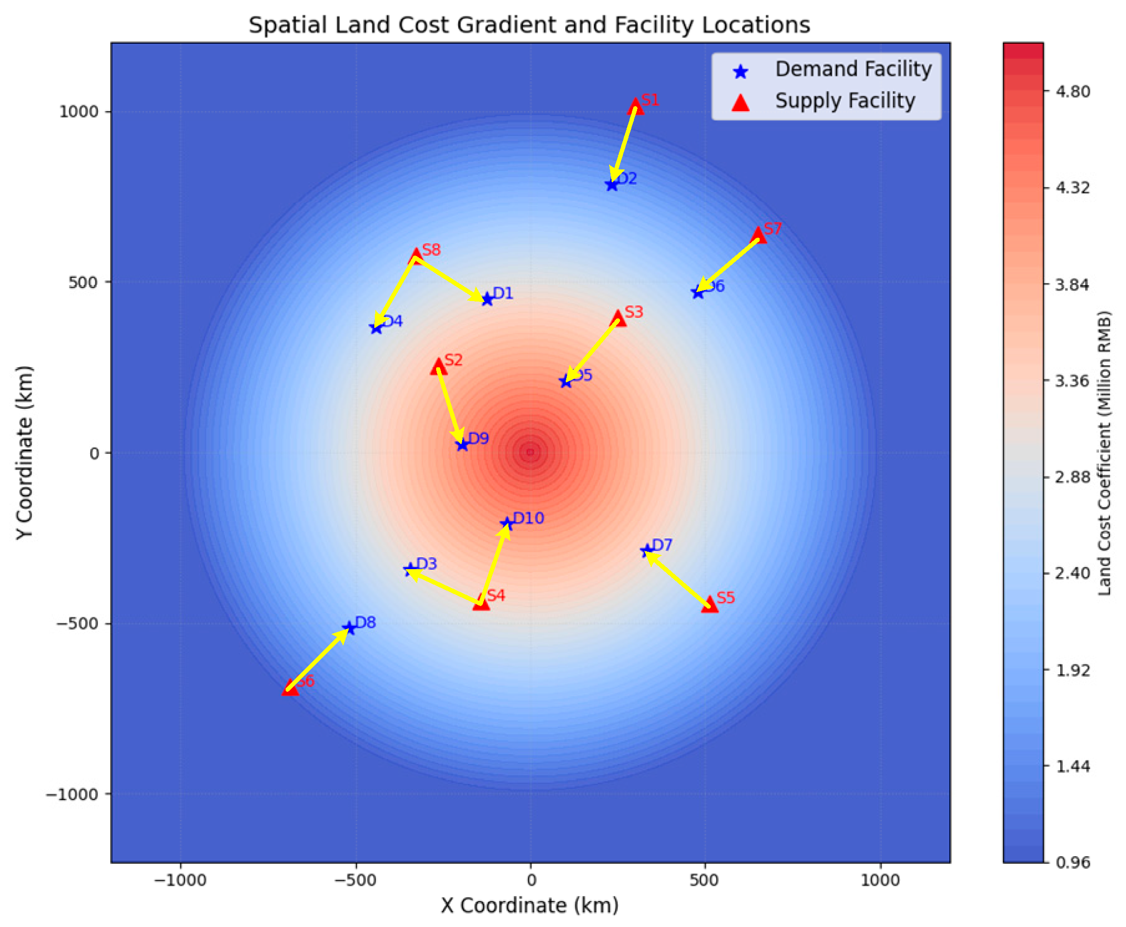
Currently, there are six existing supply stations in operation. Their spatial distribution and supply–demand relationships are detailed in Table 3 and Table 4 and illustrated in Figure 1. The total cost at this stage amounts to USD 139.96 million.
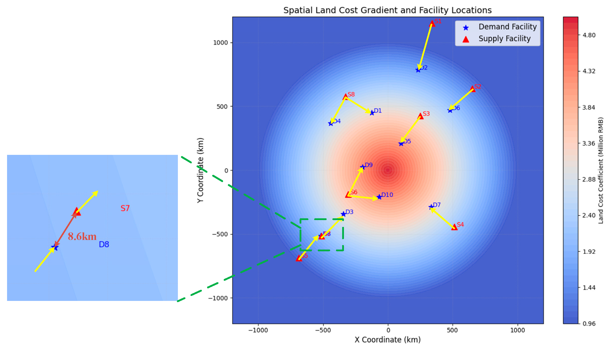
Under the constraint of maintaining the spatial locations of the existing six supply points, four additional candidate supply nodes were introduced, and the logistics supply–demand relationships and material requirements were re-optimized. The optimization of the proposed model was carried out using the DICOPT solver in GAMS 23.7 (GAMS Development Corporation, Washington, DC, USA) on a PC equipped with an Intel Core i7-14700 2.1 GHz CPU and 32 GB RAM (Intel Corporation, Santa Clara, CA, USA). The optimization results show that the most cost-efficient configuration is achieved by adding two new supply points (S7 and S8), and the spatial layout of these points, along with the redefined supply–demand relationships, significantly enhances the system’s efficiency and cost-effectiveness. Specifically, the locations of the new supply points and the optimized supply–demand matching relationships are presented in Table 5 and Table 6, with a visual representation provided in Figure 2.
Figure 1 shows the baseline layout of six supply warehouses, which is skewed toward low-cost areas and avoids high-cost areas. After introducing S7 and S8 (Figure 2), the layout becomes more balanced, especially for demand nodes such as D1 and D4. Table 3 and Table 4 provide spatial coordinates and cost parameters. The repositioning of S8 balances land costs with transportation efficiency. In Case 1, while maintaining the spatial locations of the six existing supply facilities, the model introduces up to four additional candidate supply nodes and re-optimizes the supply–demand relationships and logistics distribution. The results indicate that the system achieves the most cost-effective configuration when two additional facilities (S7 and S8) are included. After optimization, the total system cost decreased from the original USD 139.96 million to USD 126.28 million, resulting in a cost saving of approximately USD 13.68 million or 9.77%. The cost reduction is attributed not only to improved logistics routing but more importantly to the strategic siting of the new facilities in areas with lower land costs, thereby significantly reducing infrastructure investment. This outcome reflects the model’s effective use of the regional land cost gradient, enhancing overall economic efficiency without altering the original facility network. This fully demonstrates the feasibility and economics of siting the facility location under the optimization results of the model.
Meanwhile, the supply relationships were restructured accordingly. The newly added facilities S7 and S8 took over partial supply responsibilities for demand points such as D6, D1, D2, and D4, alleviating the pressure on original facilities like S2 and S3. The released capacity of the original facilities was reallocated to enable a more cost-effective logistics configuration. As shown in Table 6, the reconfigured supply–demand relationships demonstrate a more balanced resource distribution, reinforcing inter-facility coordination while enhancing the economic adaptability and robustness of the system under existing response constraints.

4.2. Case 2: Network Reconstruction Under Systemic Failure

The second case scenario considers a more extreme situation in which the existing emergency logistics system becomes non-functional due to large-scale accidents, infrastructure damage, or policy-driven restructuring. In this case, a full redesign of the emergency supply network is required, including both the spatial siting of supply facilities and the routing of resource deliveries.
This case is modeled as a complete location–routing joint optimization problem, incorporating comprehensive constraints such as safety radii, heterogeneous regional costs, storage–dispatch trade-offs, and support time windows. By solving the full-scale MINLP model, the optimized logistics configuration significantly reduces the system-wide cost while ensuring coverage and compliance. Compared with traditional sequential or decoupled models, our integrated approach yields more balanced and resilient facility distributions and routing patterns.
The region, as mentioned above, includes 10 CIPs, with their spatial coordinates and demand quantities detailed in Table 1 and Table 2. A total of ten candidate supply facility locations were pre-selected based on spatial considerations, land cost distribution, and proximity to high-demand areas. Through comprehensive model-based optimization, it was determined that introducing nine of these candidate supply nodes yielded the lowest overall system cost, representing the most economically efficient configuration. Specifically, the locations of the new supply points and the optimized supply–demand matching relationships are presented in Table 7 and Table 8, with a visual representation provided in Figure 3.
Figure 3 shows the optimized layout achieved through a comprehensive network redesign, activating nine warehouses distributed across the grid. Site selection prioritizes the low-cost area, completely avoiding high-cost core zones while adhering to an 8 km domino safety buffer zone. The full reconstruction strategy applied in Case 2 demonstrates the effectiveness of the integrated location–routing optimization model under extreme system failure conditions. By completely redesigning the spatial layout of supply facilities and their corresponding dispatch relationships, the model capitalized on both land cost gradients and supply–demand synergies. Out of ten pre-selected candidate sites, nine were ultimately activated, forming a comprehensive logistics network that ensures complete coverage while avoiding spatial conflict through strict enforcement of the 8 km minimum safety distance.
The optimized configuration resulted in a total system cost of USD 118.76 million, significantly lower than the baseline configurations of both Case 1 and traditional decoupled models. The majority of the cost savings originated from the strategic siting of facilities in low-cost zones without compromising service scope or logistical feasibility. Through sensitivity analysis, we found that land prices are the most important influencing factor.
The MINLP was first relaxed to an NLP and then solved through DICOPT’s outer-approximation cycle; the initial NLP sub-problem was feasible but non-optimal, and the first MILP master problem produced an optimal incumbent within 26 s. Subsequent scenarios of comparable size required between 22 s and 31 s, confirming that the formulation remains tractable for real-time decision support (see Table 9).

5. Discussion and Conclusions

This study proposes a unified optimization framework for emergency logistics in large-scale CIPs, addressing the core limitation of facility–routing decoupling prevalent in sequential models. By incorporating spatial safety constraints (e.g., ≥8 km minimum separation), heterogeneous land cost distributions, and multi-source dispatch within a single MINLP formulation, the model achieves significant cost reductions—9.77% in the incremental-expansion scenario and 15.10% in the network-reconstruction scenario—while maintaining complete service coverage and strict regulatory compliance.
Compared to existing two-stage heuristics (e.g., Caunhye et al., 2016 [18]) and robust siting models (e.g., Xu et al., 2024 [12]), these improvements reflect both economic and methodological advantages. Empirically, the optimized facility sites cluster in zones with lower land price gradients, validating the model’s sensitivity to spatial cost heterogeneity and reinforcing the role of siting in shaping overall system performance. From a practical standpoint, such results support a replicable “one park–one plan” approach to the emergency stockpile layout in high-risk regions.
Key innovations of this work include the following:
(a)
Scenario adaptability: The framework applies to both incremental optimization and full network redesign, offering flexibility for diverse emergency-preparedness needs.
(b)
Economic–spatial synergy: The integration of radial land cost gradients reduces infrastructure investment without compromising safety, as demonstrated in both case scenarios.
(c)
Operational resilience: By enforcing domino safety distances and dynamically reallocating supply–demand assignments, the model enhances resource utilization while adhering to spatial risk controls.
From a methodological perspective, the model demonstrates 27% faster solve times versus its sequential counterpart under the same hardware and tolerance settings, confirming the computational gains of integration. The transportation-time assumption—based on the Euclidean distance and average vehicle speed—is consistent with the prior literature and offers a tractable baseline for large-scale response modeling. Still, we acknowledge that this simplification may underestimate delays caused by real-world traffic conditions. Future extensions may incorporate network-based travel-time estimates or real-time congestion data to improve realism.
Finally, the current model adopts deterministic inputs. Incorporating parameter uncertainty (e.g., demand volatility, cost fluctuation) remains a crucial yet computationally intensive task. Future research will explore robust or scenario-based extensions to enhance the model’s adaptability under uncertainty and better reflect real-world emergency dynamics. Addressing parameter uncertainty (e.g., in demand or cost) remains an important yet computationally intensive challenge, which we plan to explore further in future model extensions.

Author Contributions

D.M. and H.Y. conceptualized the study and developed the methodology. The investigation was carried out by D.M., with D.M. and H.Y. performing the analysis and interpretation of the data. D.M. contributed to the study conceptualization, methodology development, investigation, and data analysis. H.Y. was involved in study conceptualization, methodology development, data analysis, and the literature review. M.B. contributed to data analysis, result interpretation, and the literature support. F.Y. assisted in methodology development and data collection. Z.C. provided support in data analysis and methodology development. F.L. contributed to data collection, the literature review, and methodology development. All authors have read and agreed to the published version of the manuscript.

Funding

Supported by the National Key R & D program of China (2021YFC3001200, 2023YFC3008800) and the National Natural Science Foundation of China, 52204208.

Institutional Review Board Statement

Not applicable.

Informed Consent Statement

Not applicable.

Data Availability Statement

The original contributions presented in this study are included in this article; further inquiries can be directed to the corresponding author.

Conflicts of Interest

All authors declare that there are no conflicts of interest.

Abbreviations

The following abbreviations are used in this manuscript:
SymbolDefinitionUnit
capLand cost factormillion dollars
cbpUnit emergency supplies’ purchase and management coststons·dollars−1
costpTotal emergency dispatch cost at supply point pmillion dollars
DSet of emergency supply demand points
DsdminMinimum safety distance constraint between two facilitieskm
fdloqQuantity of emergency supplies required at demand point qtons
fspTotal amount of emergency resources stored at supply point ptons
fstdp, qQuantity of emergency supplies transported from supply point p to demand point qtons
kLRate of cost decline with distancemillion dollars km−1
Land0Baseline land price at the originmillion dollars
M1Sufficiently large positive number in “Big-M”
M2Large constant to deactivate constraint when zf (p,q) = 0
M3Sufficiently large positive value
M4Small positive constant to avoid numerical instability
pEmergency supply point index
qEmergency demand point index
rsdpEuclidean distance from origin to facility locationkm
SSet of emergency supply points
sdp, qEuclidean distance between facilities p and qkm
svqEmergency supply consumption rate at demand point qtons·hour−1
tsqSupport time for stored emergency supplies at demand point qhours
TcostTotal of all supply point dispatch costsmillion dollars
Ttp, qTransportation time from p to qhours
xapHorizontal coordinate of supply facility p
xaqHorizontal coordinate of demand facility q
yapVertical coordinate of supply facility p
yaqVertical coordinate of demand facility q
zfp, qBinary variable: whether supply point p serves demand point q0 or 1
ztpBinary variable: whether supply point p is activated0 or 1

References

  1. Yang, P.; Zhang, L.; Tao, G. Smart Chemical Industry Parks in China: Current Status, Challenges, and Pathways for Future Sustainable Development. J. Loss Prev. Process Ind. 2023, 83, 105105. [Google Scholar] [CrossRef]
  2. Hou, J.; Gai, W.-M.; Cheng, W.-Y.; Deng, Y.-F. Hazardous Chemical Leakage Accidents and Emergency Evacuation Response from 2009 to 2018 in China: A Review. Saf. Sci. 2021, 135, 105101. [Google Scholar] [CrossRef]
  3. Wang, B.; Wu, C.; Reniers, G.; Huang, L.; Kang, L.; Zhang, L. The Future of Hazardous Chemical Safety in China: Opportunities, Problems, Challenges and Tasks. Sci. Total Environ. 2018, 643, 1–11. [Google Scholar] [CrossRef] [PubMed]
  4. Wu, Q.; Han, J.; Lei, C.; Ding, W.; Li, B.; Zhang, L. The Challenges and Countermeasures in Emergency Management after the Establishment of the Ministry of Emergency Management of China: A Case Study. Int. J. Disaster Risk Reduct. 2021, 55, 102075. [Google Scholar] [CrossRef]
  5. Ding, Z.; Xu, X.; Jiang, S.; Yan, J.; Han, Y. Emergency Logistics Scheduling with Multiple Supply-Demand Points Based on Grey Interval. J. Saf. Sci. Resil. 2022, 3, 179–188. [Google Scholar] [CrossRef]
  6. Kundu, T.; Sheu, J.B.; Kuo, H.T. Emergency Logistics Management—Review and Propositions for Future Research. Transp. Res. E Logist. Transp. Rev. 2022, 164, 102789. [Google Scholar] [CrossRef]
  7. Duan, W.; He, B. Emergency Response System for Pollution Accidents in Chemical Industrial Parks, China. Int. J. Environ. Res. Public Health 2015, 12, 7868–7885. [Google Scholar] [CrossRef]
  8. Du, Y.; Sun, J.; Duan, Q.; Qi, K.; Xiao, H.; Liew, K.M. Optimal Assignments of Allocating and Scheduling Emergency Resources to Accidents in Chemical Industrial Parks. J. Loss Prev. Process Ind. 2020, 65, 104148. [Google Scholar] [CrossRef]
  9. Jiang, Y.; Xu, K.; Gai, W.; Salhi, S. Emergency Response for Tackling Major Accidental Toxic Gas Releases: What Should Be Done and When? Saf. Sci. 2022, 154, 105819. [Google Scholar] [CrossRef]
  10. Xu, Z.; Zheng, C.; Zheng, S.; Ma, G.; Chen, Z. Multimodal Transportation Route Optimization of Emergency Supplies Under Uncertain Conditions. Sustainability 2024, 16, 10905. [Google Scholar] [CrossRef]
  11. Mukhopadhyay, A.; Pettet, G.; Vazirizade, S.M.; Lu, D.; Jaimes, A.; El Said, S.; Baroud, H.; Vorobeychik, Y.; Kochenderfer, M.; Dubey, A. A Review of Incident Prediction, Resource Allocation, and Dispatch Models for Emergency Management. Accid. Anal. Prev. 2022, 165, 106501. [Google Scholar] [CrossRef]
  12. Xu, F.; Ma, Y.; Liu, C.; Ji, Y. Emergency Logistics Facilities Location Dual-Objective Modeling in Uncertain Environments. Sustainability 2024, 16, 1361. [Google Scholar] [CrossRef]
  13. Wang, W.; Wu, S.; Wang, S.; Zhen, L.; Qu, X. Emergency Facility Location Problems in Logistics: Status and Perspectives. Transp. Res. E Logist. Transp. Rev. 2021, 154, 102465. [Google Scholar] [CrossRef]
  14. Boonmee, C.; Arimura, M.; Asada, T. Facility Location Optimization Model for Emergency Humanitarian Logistics. Int. J. Disaster Risk Reduct. 2017, 24, 485–498. [Google Scholar] [CrossRef]
  15. Yao, J.; Zhang, X.; Murray, A.T. Location Optimization of Urban Fire Stations: Access and Service Coverage. Comput. Environ. Urban. Syst. 2019, 73, 184–190. [Google Scholar] [CrossRef]
  16. Dantrakul, S.; Likasiri, C.; Pongvuthithum, R. Applied P-Median and p-Center Algorithms for Facility Location Problems. Expert. Syst. Appl. 2014, 41, 3596–3604. [Google Scholar] [CrossRef]
  17. Karatas, M.; Razi, N.; Tozan, H. A Comparison of P-Median and Maximal Coverage Location Models with Q-Coverage Requirement. Procedia Eng. 2016, 149, 169–176. [Google Scholar] [CrossRef]
  18. Carnero Quispe, M.F.; Couto, A.S.; de Brito Junior, I.; Cunha, L.R.A.; Siqueira, R.M.; Yoshizaki, H.T.Y. Humanitarian Logistics Prioritization Models: A Systematic Literature Review. Logistics 2024, 8, 60. [Google Scholar] [CrossRef]
  19. Akgün, I.; Gümüşbuğa, F.; Tansel, B. Risk Based Facility Location by Using Fault Tree Analysis in Disaster Management. Omega 2015, 52, 168–179. [Google Scholar] [CrossRef]
  20. Hu, H.; He, J.; He, X.; Yang, W.; Nie, J.; Ran, B. Emergency Material Scheduling Optimization Model and Algorithms: A Review. J. Traffic Transp. Eng. (Engl. Ed.) 2019, 6, 441–454. [Google Scholar] [CrossRef]
  21. Yuan, Y.; Wang, F. An Emergency Supplies Scheduling for Chemical Industry Park: Based on Super Network Theory. Environ. Sci. Pollut. Res. 2022, 29, 39345–39358. [Google Scholar] [CrossRef]
  22. Bodaghi, B.; Shahparvari, S.; Fadaki, M.; Lau, K.H.; Ekambaram, P.; Chhetri, P. Multi-Resource Scheduling and Routing for Emergency Recovery Operations. Int. J. Disaster Risk Reduct. 2020, 50, 101780. [Google Scholar] [CrossRef] [PubMed]
  23. Zhang, L.; Li, J.; Wang, J.; Yuan, N. Research on Location-Inventory-Routing Optimization of Emergency Logistics Based on Multiple Reliability under Uncertainty. Comput. Ind. Eng. 2025, 200, 110826. [Google Scholar] [CrossRef]
  24. Pu, X.; Zhao, X. Post-Earthquake Emergency Logistics Location-Routing Optimization Considering Vehicle Three-Dimensional Loading Constraints. Symmetry 2024, 16, 1080. [Google Scholar] [CrossRef]
  25. Caunhye, A.M.; Zhang, Y.; Li, M.; Nie, X. A Location-Routing Model for Prepositioning and Distributing Emergency Supplies. Transp. Res. E Logist. Transp. Rev. 2016, 90, 161–176. [Google Scholar] [CrossRef]
  26. Sun, H.; Huang, Y.; Chang, Q.; Li, J. A Robust and Multi-Period Model for an Emergency Logistics Network Considering the Risk of Disruptions. RAIRO-Oper. Res. 2025, 59, 1501–1525. [Google Scholar] [CrossRef]
  27. Liu, L.; Tian, T.; Wang, R.; Li, S. Time Varying Route Optimization of Hazardous Materials Transportation Considering Risk Equity. Preprints 2025. [Google Scholar] [CrossRef]
  28. Liu, Q.; Liu, J.; Yang, Y.; Wang, Y. Research on Optimization and Intelligent Upgrading Strategies for Emergency Logistics Systems. In Proceedings of the 2024 6th Management Science Informatization and Economic Innovation Development Conference (MSIEID 2024), Guangzhou, China, 6–8 December 2024; Atlantis Press: Dordrecht, The Netherlands, 2025; pp. 605–612. [Google Scholar] [CrossRef]
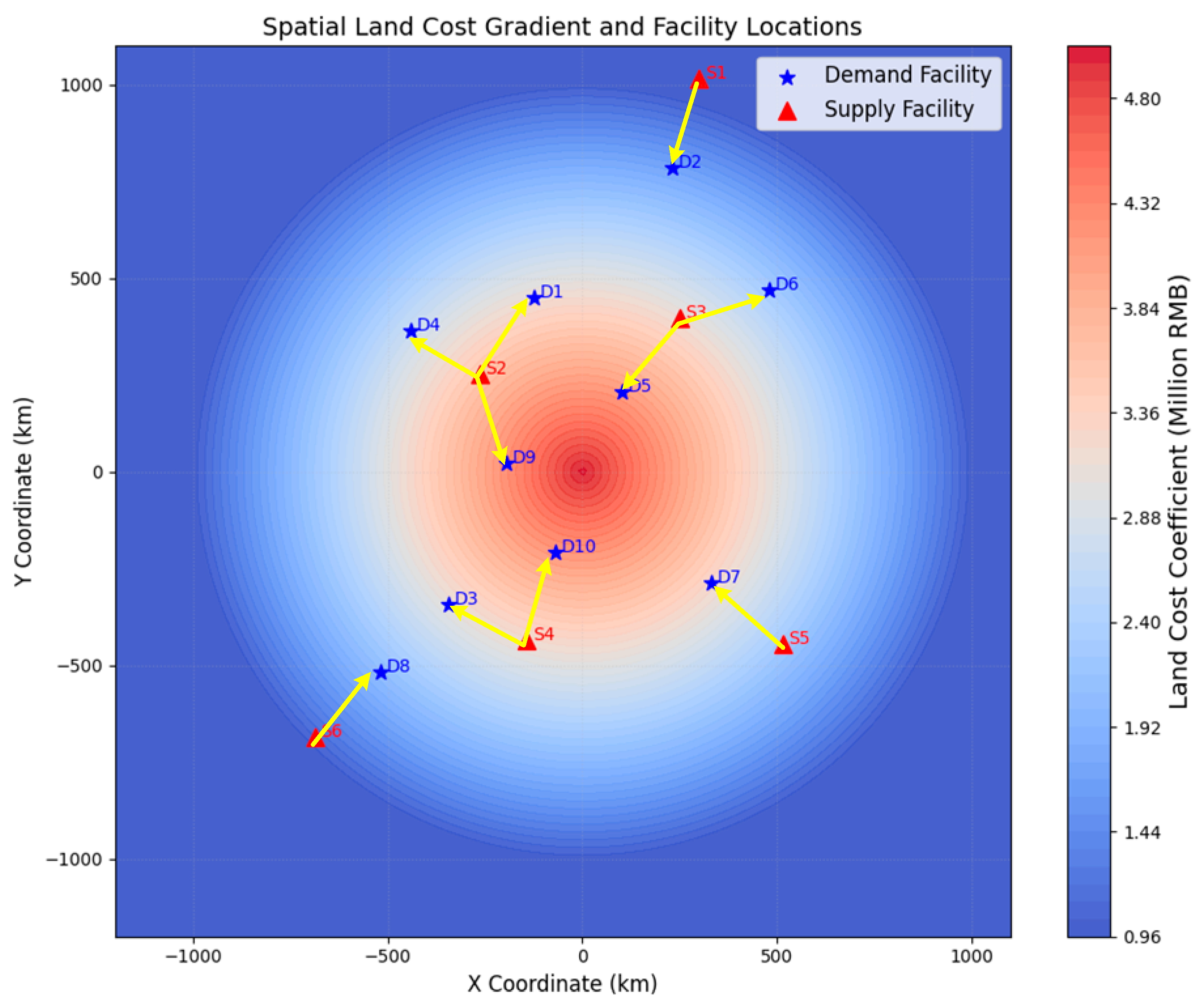
Figure 1. Land cost gradient and facility locations.
Processes 13 02513 g001
Figure 2. Land cost gradient and facility locations in case 1.
Processes 13 02513 g002
Figure 3. Land cost gradient and facility locations in case 2.
Processes 13 02513 g003
Table 1. Locations of demand facilities.
Demand Facility IDX CoordinateY Coordinate
D1−125.00450.00
D2231.00787.00
D3−343.00−344.00
D4−441.00366.00
D5101.00208.00
D6479.00469.00
D7332.00−287.00
D8−518.00−516.00
D9−195.0024.00
D10−68.00−208.00
Table 2. Parameters of demand facilities.
Demand Facility IDAdditional Emergency Supply Demand (Tons)Consumption Rate of Emergency Supplies (Tons/Hour)Self-Reserve of Emergency Supplies (Tons)
D18303090
D2105040120
D3239090270
D49803090
D53130110330
D6159060180
D7162060180
D83310120360
D9140050150
D10203070210
Table 3. Supply facility locations and inventory.
Supply Facility IDX CoordinateY CoordinateEmergency
Reserve Stockpile
S1298.591017.281050
S2−263.51254.003210
S3250.44395.794720
S4−142.58−436.124420
S5513.56−443.951620
S6−688.03−685.383310
Table 4. Supply–demand relationship and logistics volume.
D1D2D3D4D5D6D7D8D9D10
S1 1050
S2830 980 1400
S3 31301590
S4 2390 2030
S5 1620
S6 3310
Table 5. Locations of demand facilities in Case 1.
Supply Facility IDX CoordinateY CoordinateEmergency
Reserve Stockpile
S1298.591017.281050
S2−263.51254.001400
S3250.44395.793130
S4−142.58−436.124420
S5513.56−443.951620
S6−688.03−685.383310
S7650.00637.041590
S8−328.12578.141810
Table 6. Supply–demand relationship and logistics volume in Case 1.
D1D2D3D4D5D6D7D8D9D10
S1 1050
S2 1400
S3 3130
S4 2390 2030
S5 1620
S6 3310
S7 1590
S8830 980
Table 7. Locations of demand facilities in Case 2.
Supply Facility IDX CoordinateY CoordinateEmergency
Reserve Stockpile (Tons)
S1341.581200.001050
S2650.48636.901590
S3250.83423.893130
S4513.56−443.951620
S5−688.03−685.383130
S6−307.18−188.173430
S7−510.46−511.952390
S8−328.14−577.801810
Table 8. Supply–demand relationship and logistics volume in Case 2.
D1D2D3D4D5D6D7D8D9D10
S1 1050
S2 1590
S3 3130
S4 1620
S5 3130
S6 14002030
S7 2390
S8830 980
Table 9. Model and solver performance statistics.
Example
Number of equations1431
Number of variables791
Number of discrete variables116
CPU time (s)26
Disclaimer/Publisher’s Note: The statements, opinions and data contained in all publications are solely those of the individual author(s) and contributor(s) and not of MDPI and/or the editor(s). MDPI and/or the editor(s) disclaim responsibility for any injury to people or property resulting from any ideas, methods, instructions or products referred to in the content.