Abstract
With the rapid growth of renewable energy integration, power systems are facing increasing uncertainty and variability in operation. The intermittent and uncontrollable nature of wind and solar generation requires operational decisions to anticipate future fluctuations, creating strong temporal coupling across days. This leads to large-scale mixed-integer linear programming (MILP) with a large number of binary variables, which is computationally intensive—especially in year-long simulations. As a result, there is a growing need for efficient modeling approaches that can reduce complexity while preserving key temporal features. This paper proposes a temporal–spatial acceleration framework for long-term power system operation simulation. In the temporal dimension, a monthly K-means clustering algorithm is applied to reconstruct typical scenario days from 8760 h time series, preserving the characteristics of seasonal and intraday variability. In the spatial dimension, thermal units with similar characteristics are aggregated, and binary decision variables are relaxed into continuous variables, transforming the MILP into a tractable LP model, and thereby reducing computational burden. Case studies are performed based on the six-bus and the IEEE RTS-79 systems to validate the framework, being able to provide a practical solution for renewable-integrated power system planning and dispatch applications.
1. Introduction
To reduce carbon dioxide emissions and lower the consumption of fossil fuels, the proportion of installed capacities from photovoltaic and wind power units has been increasing rapidly in recent years. Nowadays, the high penetration of renewable energies has been widely integrated into modern power systems.
The output of renewable energies is highly variable and difficult to predict, which increases the complexity of system operation, and further affects the secure operation of the power systems. For example, utility-scale solar plants have shown rapid output fluctuations due to cloud transients, stressing grid frequency, and ramping capabilities, inducing challenges in scheduling [1]. Moreover, short-term wind power variations can affect the control performance of the system, leading to instability and even disconnection from the grid, causing safety issues [2]. Therefore, it is necessary to capture the fluctuation characteristics of renewable energy generation and simulate different operating scenarios of the power systems, so as to support its secure and economically optimal operation.
Most conventional temporal operation simulation methods rely on typical day modeling, which only ensures feasibility in typical days. However, the representative characteristics of typical days evolve over time. The approach, which focuses on typical day selections, is only capable of capturing a limited range of seasonal variability in energy and power fluctuations and thus fails to reflect the full-year dynamics of power system operations. Therefore, it highlights the need for high-resolution, 8760 h time series simulations to more accurately capture temporal uncertainty and variability.
While full-year hourly simulations provide higher accuracy, they also introduce significant computational challenges due to long-term temporal coupling constraints. To address these problems, researchers have explored various simplification techniques for time series modeling in systems with high renewable penetration. These techniques generally fall into two categories. (1) The multi-timescale grid method [3,4]: The multi-timescale grid method models different types of devices in power systems based on temporal grids corresponding to various timescales. Ref. [5] applies the multi-timescale grid method to analyze the charging and discharging behavior of long-term and short-term energy storage systems. Ref. [6] proposes a unified hierarchical multi-timescale grid method for the optimal allocation of flexibility resources in power systems. (2) Time series clustering method [7,8]: Ref. [9] used time series aggregation to replace a full hourly or even sub-hourly PSOM (Power System Optimization Model) with a smaller model using a simplified time dimension. Ref. [10] proposed a short-term load forecasting method that combines K-shape time series clustering with graph convolutional networks, identifying user groups with similar electricity usage habits. Ref. [11] employed the Dynamic Time Warping (DTW) method to conduct a cluster analysis of the time series of renewable energy in 130 countries in order to evaluate the similarities and differences in their usage patterns.
Although these methods have compressed a large number of scenarios in terms of time sequence and reduced the computational burden, they lose many fluctuation features and are unable to accurately simulate the annual fluctuation characteristics of new energy and load. Preserving daily and seasonal cycles in both renewable generation and load profiles is essential for accurately modeling their annual temporal characteristics, as these cycles are driven by intrinsic natural and behavioral factors [10,12,13]. When considering the time series scenario compression method, it is necessary to consider how to extract and retain the short-term and seasonal characteristics.
In the spatial dimension, the large number of binary variables associated with thermal generators significantly increases the computational burden, especially in year-long sequential simulations. To reduce this complexity, various methods have been proposed, including binary variable relaxation [14,15] and rolling horizon techniques [16,17]. Some studies incorporate flexible temporal resolution or operational flexibility to simplify the problem structure, reducing the MILP to a linear program [18,19]. Others focus on unit clustering, aggregating similar generators to lower the model dimensionality [20,21]. While these spatial simplifications improve computation time, they often compromise accuracy, especially when system security and stability constraints are considered.
To address the above challenges, in the process of conducting the annual optimization operation simulation of the power system, it is essential to capture and preserve both short-term and seasonal characteristics in temporal scenario compression, while ensuring fast and accurate computation under security and stability constraints in the spatial dimension. Therefore, in this article, aiming at full-year hourly optimization operation simulations, we propose monthly K-means clustering and the reconstruction of representative scenario days to reduce the temporal dimensionality while retaining key temporal features. Moreover, in the spatial dimension, we introduce a spatial acceleration strategy that aggregates generating units with similar operational characteristics and applies linear relaxation techniques to reduce the complexity associated with binary decision variables. Table 1 and Table 2 present the main temporal and spatial simplification methods, respectively, showing their key features, advantages, and limitations. These comparisons help highlight the positioning and strengths of the proposed framework relative to existing approaches. Compared to traditional approaches, the proposed method preserves both seasonal and intraday variability in time, while achieving substantial binary variable reduction through spatial aggregation, enabling practical large-scale system simulations.

Table 1.
Comparison of temporal simplification methods.
Table 2.
Comparison of spatial simplification methods.
The rest of this paper is structured as follows. Section 2 introduces the temporal acceleration algorithm. Section 3 presents the spatial acceleration algorithm. Section 4 presents numerical simulations on a six-bus system and the modified RTS79 test system to evaluate the accuracy and computational efficiency of the proposed framework. Finally, Section 5 draws the conclusion.
2. Temporal Acceleration Algorithm
2.1. Operation Simulation Model Based on 8760-Hour Time Series
For power systems with high proportion of renewable energy, full-year operational simulation models with large-scale temporal coupling are needed to accurately capture system dynamics, whereas traditional day-averaged simulations only ensure intra-day balance but fail to reflect long-term variations. At present, many studies have proposed 8760 h hourly operational simulations to accurately capture annual temporal fluctuations. This links daily load profiles and renewable output curves into time-coupled constraints, enabling system states to be tracked on an hourly basis.
However, performing a continuous simulation of power system operations over an entire year (8760 h) leads to a large-scale mixed-integer linear programming (MILP) problem, which significantly increases computational complexity. Therefore, in this section, we propose applying monthly K-means clustering and reconstructing representative scenario days to reduce the temporal dimensionality while preserving key temporal features.
2.2. Time Series Acceleration Algorithm
The acceleration algorithm for source-load time series data is illustrated in Figure 1, and the implementation process is elaborated step by step as follows. Additionally, our study assumes that, for each actual calendar day represented by a given typical day, the power system’s operational state—including the on/off status of generating units and load demand—remains consistent across the same time intervals throughout the day.
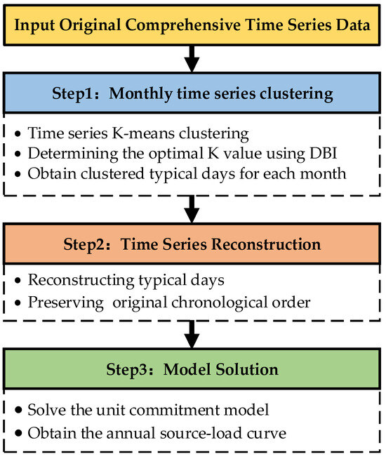
Figure 1.
Time series acceleration flow chart.
- Step 1: Monthly Time Series Clustering
To extract typical daily patterns from wind power generation and load demand data, this study applies the K-means clustering algorithm to perform monthly clustering. Each data sample represents a 24 h time series, capturing the intraday variation in wind generation and load demand.
The procedure begins by specifying the number of clusters, K, which typically ranges from 2 to 7 for each month. Next, K samples are randomly selected as the initial centroids. Each day is assigned to the nearest cluster based on the Euclidean distance between its 24 h profile and the corresponding cluster centroids. The centroids are then updated by averaging all-time series within each cluster. This process is repeated until the cluster assignments converge and remain stable no longer change significantly.
K-means enables a clear partition of the dataset into representative daily patterns and reveals structural similarities in wind generation and load demand, supporting forecasting, operational planning, and reliability analysis in power systems.
DBI:
Within this framework, Formula (2) denotes the number of intra-cluster data points whose distances to the corresponding cluster centroids are less than the cluster radius, thereby indicating the internal density of the cluster. Conversely, Formula (3) represents the number of data points located between any two clusters, where their distances to the midpoint between clusters are smaller than the average cluster radius. This reflects the density of data in the inter-cluster region.
To determine the optimal number of clusters, K, for each month’s time series using K-means clustering, we apply the Davies–Bouldin Index (DBI). The value of K that minimizes the DBI corresponds to the most appropriate clustering structure for selecting representative scenario days.
Compared with the traditional method that relies on the Sum of Squared Errors (SSE) to determine K, the DBI-based approach offers two key advantages: (1) it helps identify the optimal number of clusters; (2) it reflects the compactness within clusters as well as the separation between them. This offers insights into monthly internal consistency and inter-month variation. As a result, this approach more effectively reflects the seasonal characteristics of wind, solar, and load time series data as well as their distribution patterns in practical scenarios. It is important to note that the optimal K value varies monthly, reflecting both seasonal dynamics of wind generation and monthly shifts in data dispersion.
- Step 2: Time Series Reconstruction
The clustered typical days are reconstructed while preserving their original chronological order, maintaining alignment with actual calendar days. This approach ensures temporal consistency with natural day sequences, keeping system operating conditions coherent at corresponding time points.
- Step 3: Model Solution
The operating cost of each generator is linearized in segments, following the method described in Ref. [22]. The simplified and reconstructed time series is subsequently utilized to solve the unit commitment model.
This approach reduces the computational load by avoiding the need to simulate every individual day. At the same time, it preserves the main temporal features and operational variability of the power system, maintaining a balance between accuracy and efficiency.
3. Spatial Acceleration Algorithm
The operational constraints of thermal power units involve numerous binary (0–1) variables. The unit commitment problem in power systems involves time-coupled 0–1 binary variables representing generator on/off states, which makes solving large-scale UC problems computationally intractable. To mitigate this challenge, we propose a spatial clustering method for computational acceleration, building upon the traditional unit commitment framework. It introduces a dispatch model and an aggregated unit model to simplify constraints. First, units with similar operating characteristics are grouped into aggregated clusters. Then, unified ramping and start–stop constraints are applied to each cluster. Finally, the binary start–stop variables are linearized into start–stop capacity parameters. This method effectively reduces the dimensionality and complexity of the model by simplifying the handling of binary variables [23].
The acceleration algorithm for spatial dimensions is shown in Figure 2, and the implementation process will be elaborated in detail as follows.
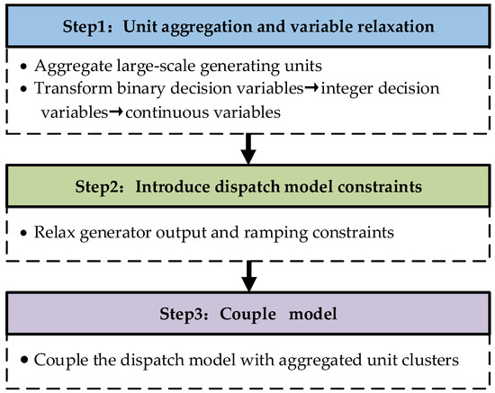
Figure 2.
Spatial clustering schematic diagram.
- Step 1: Unit aggregation and variable relaxation
First, all generating units in the classical unit commitment problem are clustered according to their operational characteristics. In this paper this characteristic refers to the maximum output power of thermal generating units. The decision variables associated with individual units are then replaced by aggregated variables representing the clustered unit groups. This approach reformulates the binary variables—which are used to indicate unit commitment and startup/shutdown status, into integer variables—.
Then, the integer decision variables are replaced with the non-negative continuous variables , representing the online capacity, startup capacity, and shutdown capacity of thermal unit cluster c. This couples the binary status/startup–shutdown variables with continuous cluster capacity variables, converting the mixed-integer linear programming (MILP) problem into a simpler linear programming (LP) problem.
The specific mathematical model is formulated as follows.
Objective Function:
The cost function of the conventional unit commitment model includes startup costs, variable operating costs, and load shedding penalty costs. represent the startup and shutdown costs per MW for thermal unit cluster c. represent the startup and shutdown status variables of the thermal unit cluster. represents the variable operating cost of thermal unit g. is the power output (MW) of thermal unit g. represents the penalty coefficient for necessary load shedding in the system. represents the necessary load shedding variable at node n in the system.
Constraints
Power balance constraint:
represent the total number of thermal units, wind units, photovoltaic units, and nodes, respectively.
Line capacity safety constraint:
G(k), W(k), V(k), L(k) represent the number of thermal units, wind units, photovoltaic units, and loads at node k. denotes the maximum allowable power flow limit of line l under normal operating conditions.
DC power flow constraints:
are the node-branch, node-thermal generator, node-wind generator, node- photovoltaic generator, and node-load matrix elements of line l, respectively. is the active power flow on branch l (with n as the power flow starting point and m as the power flow ending point).
Renewable output robustness constraints:
To represent the uncertainty of wind and photovoltaic generation, we define the output ranges and , which characterize the power uncertainty intervals at each time step t.
represent the lower and upper bounds of wind and photovoltaic power outputs at time t, respectively. These intervals reflect the uncertainty ranges of renewable generation and form the robust uncertainty set used in the dispatch problem.
Power output limit constraints:
is the minimum output rate of thermal power. First, instead of modeling the on/off statuses of individual units, the online capacity of unit cluster c is formulated and captured as , where denotes the number of on-line units within unit cluster c at time period t. is the average capacity of the units in unit cluster c. Next, integrate the cluster capacity and the operating status of the cluster into a single variable. Replace with the continuous variable to represent the online capacity within cluster c.
Ramping constraints:
and represent the hourly up and down ramp rates for thermal unit, respectively. The formulation is transformed in the same manner as the power output constraints described above.
Linkage between operational variables and startup/shutdown variables:
represent the integer startup and shutdown variables of cluster c at time t, respectively. Specifically, for individual generating units, their operating status is represented by a binary variable , where indicates that unit g is online at time t and 0 otherwise. In the clustered model, units with similar characteristics are aggregated into cluster c, and an integer variable is used to represent the number of online units in cluster c at time t, where denotes the total number of units in cluster c. Subsequently, these integer variables are integrated with unit capacity and reformulated as continuous variables to represent the total online capacity and startup/shutdown capacity of each cluster. This transformation enables a shift from a nonlinear to a linear formulation, improving the computational efficiency of the model.
Minimum startup time constraints:
Formula (11) represents the conventional startup and shutdown constraints for individual generating units in traditional unit commitment formulations. After clustering, the corresponding constraints are reformulated for each cluster c, as shown in Formula (12), which captures the startup and shutdown behavior in terms of the number of units operating or starting up within each cluster.
On the basis of the above, the integer variable is replaced by the continuous variable as described in the power output limits constraints. This transformation integrates unit count and capacity into a single variable. As a result, the constraints are reformulated into a capacity-based representation. The minimum up-time requirement is then expressed in terms of the online capacity, as shown in Formula (13).
Minimum shutdown time constraints:
The minimum down-time constraint can be derived in a similar manner to the minimum up-time constraint discussed above. The corresponding formulation is formulated as follows:
The aggregated model retains standard unit commitment formulations, simply replacing individual unit indices with cluster index c. Since all units within a cluster are assumed identical, their characteristic parameters (e.g., unit capacity, minimum load ratio, ramp rate, and minimum up/down time) are defined as cluster averages. For example, represents the average capacity of units in cluster c, calculated as . Other cluster parameters follow the same averaging principle. Additionally, indicates the required continuous operation/downtime duration at daily initialization for each cluster, subject to constraints and .
- Step 2: Introduce dispatch model constraints
Generator output and ramping constraints are relaxed by adding critical assumptions for thermal units:
- ①
- Flexibility: Thermal units can adjust power output without limits (from zero to full capacity), ignoring minimum generation thresholds.
- ②
- Instant response: Units achieve immediate startup/shutdown with negligible command-delay.
- Step 3: Model Coupling
Ensure the total output power of all thermal units in each cluster equals the input defined by the dispatch model.
4. Case Studies
4.1. Six-Bus System
After inputting the original wind power time series data, we apply K-means clustering to the time series of each individual month. This procedure allows us to extract several representative days for each month. These representative days effectively retain short-term diurnal variations while also reflecting the monthly level fluctuation patterns of the system. Subsequently, we reconstruct and merge these representative days to form a new time series that approximates the original data. By sequentially reconstructing the scenario days from the original dataset, we enable a comprehensive simulation of power system operation over time using the newly formed time series.
To demonstrate the effectiveness of this method, a six-bus system is used as the testbed. As shown in Figure 3, the test system consists of 6 key buses, interconnected by 13 transmission lines, and equipped with 4 generating units—comprising 3 thermal generators and 1 wind power unit. For easy understanding, the configuration data for the six-bus system are provided in Table A1.
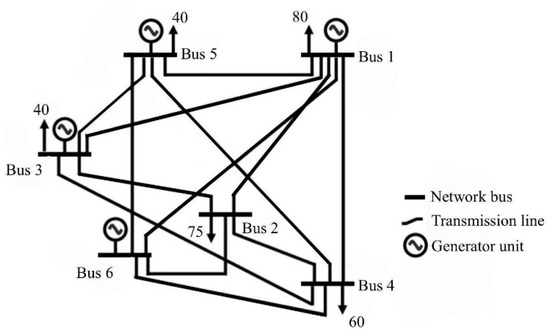
Figure 3.
Six-bus test system.
The proposed scheme (labeled as Scheme 3) is compared with two classical approaches (each scheme has been integrated into the spatial acceleration method):
- Hourly operational simulation based on the original 8760 h time series (basic scheme);
- Clustering the annual time series using K-means, then reconstructing the representative days based on the clustering results, and conducting operational simulation based on the reconstructed time series.
Figure 4 presents the optimal clustering results for each month as determined by the proposed approach. The number of representative days differs across months, with June, September, and December showing relatively higher values (5 days), indicating greater variability and randomness in the time series during those periods.
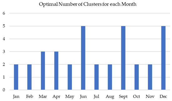
Figure 4.
Monthly optimal number for clusters.
Table 3 compares the performance of each scheme in terms of unit generation, generation cost, number of optimization variables, and solution time, with a solution gap of no more than 0.03%. All schemes exhibit small errors in total annual generation, with Scheme 2 achieving the lowest annual error of 1.0%. However, for intra-day operations, Scheme 2 shows a significantly larger error of up to 30.4%. In contrast, Scheme 3 maintains low error levels at both the annual and daily scales, with deviations of 2.3% and 0.4%, respectively, indicating high accuracy in modeling thermal generation. In terms of generation cost, both Schemes 2 and 3 yield similarly small deviations. Notably, Scheme 3 substantially reduces the number of optimization variables—only 10,082, compared to 140,227 in Scheme 1 and 44,749 in Scheme 2—greatly simplifying the problem. Moreover, Scheme 3 achieves the shortest solution time of 161 s, reflecting a significant improvement in computational efficiency.
Table 3.
Comparison of simulation results under three schemes.
Considering all aspects, Scheme 3 shows significant advantages for improving optimization efficiency while maintaining acceptable solution accuracy. These findings confirm the effectiveness of the operational simulation method proposed in this work.
Figure 5 illustrates the thermal power output profiles under the three schemes for a typical day. Figure 6 shows the monthly thermal generation across the year. In Figure 5, Scheme 2 significantly underestimates thermal generation during several hours. This output deviation is mainly due to its failure to capture the synchronous peaks in load and dips in renewable output—especially when high demand coincides with low renewable availability. In contrast, Scheme 3 closely tracks the hourly profile of Scheme 1, indicating that it successfully retains key temporal dynamics despite data reduction. Figure 6 further confirms this over the annual scale. Scheme 2 underestimates thermal generation in several months, most notably in July and August, where system reliability heavily depends on thermal support due to high load and volatile renewable output. Scheme 3, however, remains highly consistent with Scheme 1 across all months, demonstrating its ability to accurately capture the interaction between load and renewable variability.
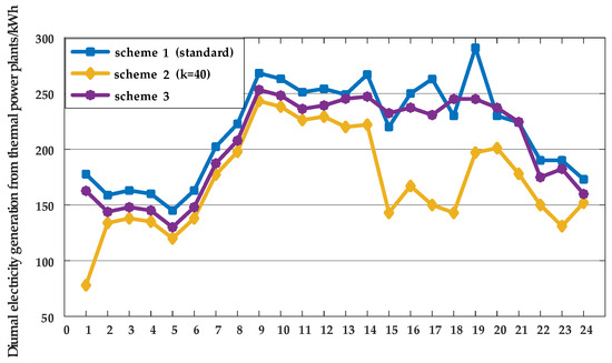
Figure 5.
Hourly thermal output on a typical day.
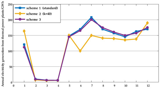
Figure 6.
Monthly thermal generation throughout the year.
Overall, the simulation outcomes clearly demonstrate that Scheme 3 achieves a balance between modeling accuracy and computational efficiency. It effectively captures the key temporal characteristics of both load and renewable generation while significantly reducing data volume and solution time, offering a more dependable foundation for power system operation and planning.
4.2. RTS79 System
To further validate the effectiveness of the proposed method, we conduct simulation experiments using the RTS79 system. To better reflect large-scale renewable integration in modern power systems, we modify the generator configuration. The updated generation portfolio includes 32 thermal units, along with 3 wind power units connected at buses 1, 21, and 23, and 3 photovoltaic units connected at buses 2, 22, and 23. All other system data remain unchanged, following the original IEEE Reliability Test System (RTS) setup [24]. The transmission network consists of 24 load/generation buses connected by 38 lines or autotransformers, operating at 138 kV and 230 kV. The topology of the RTS 79 system is shown in Figure 7.
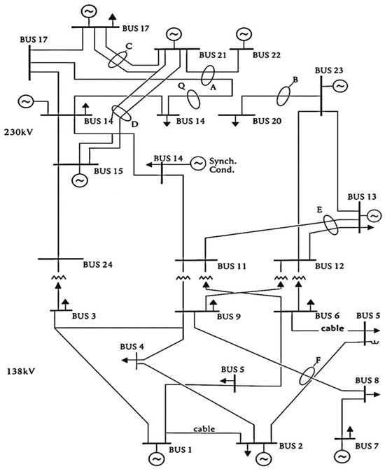
Figure 7.
RTS 79 system.
After applying monthly clustering to the time series within the RTS79 system, the results, as illustrated in the corresponding Figure 8, show that June exhibits the highest daily variability, with up to six representative days.
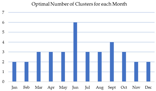
Figure 8.
Monthly optimal number for clusters.
Table 4 summarizes the simulation results of different schemes, all solved with a gap below 1%. Scheme 1, based on the full 8760 h time series, serves as the benchmark with zero cost error but incurs the highest computation time. In Scheme 2, increasing the number of clusters reduces the generation cost error but significantly increases solving time. Among them, the best accuracy (4.3%) is achieved when k = 120, but at a high cost of 2880 s. In contrast, Scheme 3 achieves a low cost error of 1.1% within 684 s of computation, offering a better trade-off between accuracy and efficiency. These results confirm the effectiveness of the proposed modeling approach.
Table 4.
Comparison of simulation results under three schemes.
4.3. Practical Large-Scale System Validation
To demonstrate the scalability of the proposed framework in practical power systems, we further apply our method to a large-scale real-world system based on data from a certain area in China. This system consists of 14,329 buses, over 1500 load buses, and spans a wide range of voltage levels from 0.04 kV to 1050 kV, covering regional backbones and local distribution grids. Due to confidentiality and privacy concerns, the detailed system topology and specific data are not disclosed. This system size significantly exceeds the RTS-79 benchmark and involves complex topologies and operational constraints under high renewable penetration.
For renewable energy configuration, the system includes the following:
- A total of 300 wind farms, with a total installed capacity of 20.06 GW;
- A total of 80,000 distributed PV plants, with a total installed capacity of 23.38 GW.
These configurations have been moderately simplified in the model to ensure computational tractability while retaining key spatial and temporal characteristics of renewable integration.
The results, illustrated in Table 5, demonstrate that the proposed temporal–spatial acceleration approach maintains high modeling accuracy while significantly reducing computational time, even under large-scale system settings. As shown in Table 3, the deviation in annual thermal generation and operational cost remains below 4% and 2%, respectively. More importantly, the proposed framework reduces the solution time of full-year optimization from 132,763 s to 4876 s, achieving a 27-fold acceleration, while maintaining a tight solution gap of 1%. These findings confirm the practicality of our method when applied to provincial- or inter-regional power systems.
Table 5.
Comparison of simulation accuracy and efficiency.
Therefore, although the case studies in Section 4.1 and Section 4.2 are based on the six-bus and RTS-79 systems, we emphasize that the same acceleration framework is also applicable to much larger systems, and the improvement in efficiency becomes even more prominent as system size increases. The performance observed in the small and medium test systems can thus be reliably extended to practical systems involving thousands of buses and generators.
5. Conclusions
This paper proposes a temporal–spatial acceleration framework to address the computational challenges in full-year operational simulations of power systems with high renewable energy penetration. The approach combines monthly K-means clustering to compress 8760 h time series data and unit aggregation with linear relaxation to reduce the binary dimensionality in unit commitment models. The proposed method preserves key seasonal and intraday variability, and reasonably simplifies the traditional model into a linear formulation, significantly reducing the computational complexity of full-year simulations.
The proposed method has been validated on both benchmark and large-scale systems. Compared with baseline approaches, it achieves high modeling accuracy while significantly reducing the number of variables and computation time. For example, in the six-bus and RTS-79 test systems, the method reduces solution time by over 90%, with cost and generation errors below 2.5%. In a real-world case with over 14,000 buses, it achieves a 27-fold acceleration while keeping key indicators within acceptable error margins.
Nonetheless, the framework has certain limitations. Firstly, unit aggregation is currently based solely on installed capacity, which may overlook operational heterogeneity. Secondly, the model does not yet include flexibility resources such as energy storage and demand response. These aspects will be addressed in future work to improve the model’s realism and applicability.
Author Contributions
Conceptualization, C.Z. and Y.Z. (Yijia Zhou); methodology, C.Z.; validation, C.Z.; formal analysis, C.Z.; writing—original draft preparation, C.Z.; writing—review and editing, Y.Z. (Yirui Zhao) and M.Y.; project administration, C.W. and Z.L. All authors have read and agreed to the published version of the manuscript.
Funding
This paper was funded by the Science and Technology Project of Central China Branch of State Grid Corporation of China, grant number 52140024000A.
Data Availability Statement
The original contributions presented in the study are included in the article; further inquiries can be directed to the corresponding author.
Conflicts of Interest
Authors Chen Wang and Zhiqiang Lu were employed by Central China Branch of State Grid Corporation of China. The remaining authors declare that the research was conducted in the absence of any commercial or financial relationships that could be construed as a potential conflict of interest. The Central China Branch of State Grid Corporation of China had no role in the design of the study; in the collection, analyses, or interpretation of data; in the writing of the manuscript, or in the decision to publish the results.
Appendix A
Table A1.
Six-bus system configuration summary.
Table A1.
Six-bus system configuration summary.
| Component | Details |
|---|---|
| Base MVA | 100 MVA |
| Number of Buses | 6 |
| Generator Capacities | G1: 40–200 MW, G2: 36–180 MW, G3: 30–150 MW |
| Generator Cost Function | Quadratic cost functions with 3-piece linearization |
| Ramp Rate | UR: 60% of Pmax, DR: 50% of Pmax |
| Renewable Profile | 1 wind farm (400 MW peak) with hourly variation |
| Load Profile | 24 h profile defined by per-unit scaling of base loads |
Table A2.
Summary of key parameters used in the optimization model.
Table A2.
Summary of key parameters used in the optimization model.
| Parameter | Description | Role in the Model |
|---|---|---|
| Thermal generator output limits | Minimum and maximum generation capacity of each thermal unit | Define the operational boundaries of thermal units |
| Startup and shutdown cost | Cost incurred when a unit starts up or shuts down | Affects overall generation cost and unit scheduling decisions |
| Ramp rate limits | Maximum allowable increase or decrease in unit output per hour | Models the flexibility of thermal units to adjust output |
| Minimum up and down time | Minimum number of hours a unit must remain on or off once started or shut down | Ensures realistic unit cycling behavior |
| Clustered unit capacity | Average capacity of thermal units within each aggregated group | Used to model the output and constraints of unit clusters |
| Wind power forecast range | Expected upper and lower bounds of wind power generation | Captures forecast uncertainty for robust dispatch |
| Photovoltaic power forecast range | Expected upper and lower bounds of photovoltaic generation | Same as above, applied to solar energy sources |
| Transmission line capacity | Maximum power flow allowed through each line | Ensures secure network operation under flow constraints |
| Network topology data | Information on how buses and lines are connected | Supports power flow calculation using network structure |
| Cluster status indicators | Continuous variables representing online capacity and transitions | Used to replace binary unit on/off states and reduce model complexity |
References
- Mills, A.; Wiser, R. Implications of Wide-Area Geographic Diversity for Short-Term Variability of Solar Power. Renew. Energy 2010, 35, 14–20. [Google Scholar] [CrossRef]
- Wang, T.; Shen, Z.; Cai, L.; Zhu, Y. A Research for the Information Loss and Its Influence of Wind Power Fluctuations in Different Time Intervals. Sustain. Energy 2016, 6, 51–61. [Google Scholar] [CrossRef]
- Boroojeni, K.G.; Amini, M.H.; Bahrami, S.; Iyengar, S.S.; Sarwat, A.I.; Karabasoglu, O. A novel multi-time-scale modeling for electric power demand forecasting: From short-term to medium-term horizon. Electr. Power Syst. Res. 2017, 142, 58–73. [Google Scholar] [CrossRef]
- Yang, Y.; Yang, P.; Zhao, Z.; Lai, L.L. A multi-timescale coordinated optimization framework for economic dispatch of micro-energy grid considering prediction error. IEEE Trans. Power Syst. 2023, 39, 3211–3226. [Google Scholar] [CrossRef]
- Renaldi, R.; Friedrich, D. Multiple time grids in operational optimisation of energy systems with short- and long-term thermal energy storage. Energy 2017, 133, 784–795. [Google Scholar] [CrossRef]
- Lin, J.; Zhang, H.; Song, Y.; Chen, G.; Ding, L.; Liang, D. Optimal investment of electrolyzers and seasonal storages in hydrogen supply chains incorporated with renewable electric networks. IEEE Trans. Sustain. Energy 2019, 11, 1773–1784. [Google Scholar] [CrossRef]
- Rager, J.M.F. Urban Energy System Design from the Heat Perspective Using Mathematical Programming Including Thermal Storage; Swiss Federal Technology Institute of Lausanne (EPFL): Lausanne, Switserland, 2015. [Google Scholar]
- Huang, Z.; Hao, H.; Du, L. Exploring the Explainability of Time Series Clustering: A Review of Methods and Practices. In Proceedings of the Eighteenth ACM International Conference on Web Search and Data Mining, Hannover, Germany, 10–14 March 2025; pp. 1005–1007. [Google Scholar] [CrossRef]
- Wu, Z.; Mu, Y.; Deng, S.; Li, Y. Spatial–temporal short-term load forecasting framework via K-shape time series clustering method and graph convolutional networks. Energy Rep. 2022, 8, 8752–8766. [Google Scholar] [CrossRef]
- Guo, W.; Li, Z.; Yin, J.; Chen, L.; Ju, P. Load profile clustering analysis based on variable density processing of time series. Power Eng. Technol. 2024, 43, 21–32. [Google Scholar]
- Maharaj, E.A.; De Giovanni, L.; D’uRso, P.; Bhattacharya, M. Deployment of renewable energy sources: Empirical evidence in identifying clusters with dynamic time Warping. Soc. Indic. Res. 2024, 175, 741–762. [Google Scholar] [CrossRef]
- Duffner, F.; Wentker, M.; Greenwood, M.; Leker, J. Battery cost modeling: A review and directions for future research. Renew. Sustain. Energy Rev. 2020, 127, 109872. [Google Scholar] [CrossRef]
- Xiao, L.; Qian, Y.; Pan, S. A relaxation method for binary optimizations on constrained Stiefel manifold. arXiv 2023, arXiv:2308.10506. [Google Scholar] [CrossRef]
- Bartmeyer, P.M.; Lyra, C. A new quadratic relaxation for binary variables applied to the distance geometry problem. Struct. Multidiscip. Optim. 2020, 62, 2197–2201. [Google Scholar] [CrossRef]
- Constante-Flores, G.E.; Conejo, A.J.; Qiu, F. AC network-constrained unit commitment via relaxation and decomposition. IEEE Trans. Power Syst. 2021, 37, 2187–2196. [Google Scholar] [CrossRef]
- Ning, X.; Chen, L.; Ma, L.; Si, Y. A Rolling Horizon Optimization Framework for Resilient Restoration of Active Distribution Systems. Energies 2022, 15, 3096. [Google Scholar] [CrossRef]
- Bischi, A.; Taccari, L.; Martelli, E.; Amaldi, E.; Manzolini, G.; Silva, P.; Campanari, D.; Macchi, E. A rolling-horizon optimization algorithm for the long term operational scheduling of cogeneration systems. Energy 2019, 184, 73–90. [Google Scholar] [CrossRef]
- Tziovani, L.; Asprou, M.; Ciornei, I.; Kolios, P.; Hadjidemetriou, L.; Lazari, A.; Tapakis, R.; Timotheou, S. Long-Term Unit Commitment with Combined-Cycle Units. In Proceedings of the 2023 IEEE Belgrade PowerTech, Belgrade, Serbia, 25–29 June 2023; pp. 01–06. [Google Scholar] [CrossRef]
- Palmintier, B. Incorporating Operational Flexibility into Electric Generation Planning: Impacts and Methods for System Design and Policy Analysis. Ph.D. Dissertation, Engineering Systems Division, MIT, Cambridge, MA, USA, February 2013. [Google Scholar]
- Yu, Z.; Zhong, H.; Ruan, G.; Yan, X. Network-Constrained Unit Commitment With Flexible Temporal Resolution. IEEE Trans. Power Syst. 2025, 40, 73–84. [Google Scholar] [CrossRef]
- Meus, J.; Poncelet, K.; Delarue, E. Applicability of a clustered unit commitment model in power system modeling. IEEE Trans. Power Syst. 2017, 33, 2195–2204. [Google Scholar] [CrossRef]
- Palmintier, B.S.; Webster, M.D. Heterogeneous unit clustering for efficient operational flexibility modeling. IEEE Trans. Power Syst. 2013, 29, 1089–1098. [Google Scholar] [CrossRef]
- Du, E.; Zhang, N.; Kang, C.; Xia, Q. A high-efficiency network-constrained clustered unit commitment model for power system planning studies. IEEE Trans. Power Syst. 2018, 34, 2498–2508. [Google Scholar] [CrossRef]
- Subcommittee, P.M. IEEE reliability test system. IEEE Trans. Power Appar. Syst. 1979, PAS-98, 2047–2054. [Google Scholar] [CrossRef]


Disclaimer/Publisher’s Note: The statements, opinions and data contained in all publications are solely those of the individual author(s) and contributor(s) and not of MDPI and/or the editor(s). MDPI and/or the editor(s) disclaim responsibility for any injury to people or property resulting from any ideas, methods, instructions or products referred to in the content. |
© 2025 by the authors. Licensee MDPI, Basel, Switzerland. This article is an open access article distributed under the terms and conditions of the Creative Commons Attribution (CC BY) license (https://creativecommons.org/licenses/by/4.0/).