Abstract
The synthesis of “green ammonia” from “green hydrogen” represents a critical pathway for renewable energy integration and industrial decarbonization. This study investigates the green ammonia synthesis process using an axial–radial fixed-bed reactor equipped with three catalyst layers. A simplified two-dimensional physical model was developed, and a multiscale simulation approach combining computational fluid dynamics (CFD) with physics-informed neural networks (PINNs) employed. The simulation results demonstrate that the majority of fluid flows axially through the catalyst beds, leading to significantly higher temperatures in the upper bed regions. The reactor exhibits excellent heat exchange performance, ensuring effective preheating of the feed gas. High-pressure zones are concentrated near the top and bottom gas outlets, while the ammonia mole fraction approaches 100% near the bottom outlet, confirming superior conversion efficiency. By integrating PINNs, the prediction accuracy was substantially improved, with flow field errors in the catalyst beds below 4.5% and ammonia concentration prediction accuracy above 97.2%. Key reaction kinetic parameters (pre-exponential factor k0 and activation energy Ea) were successfully inverted with errors within 7%, while computational efficiency increased by 200 times compared to traditional CFD. The proposed CFD–PINN integrated framework provides a high-fidelity and computationally efficient simulation tool for green ammonia reactor design, particularly suitable for scenarios with fluctuating hydrogen supply. The reactor design reduces energy per unit ammonia and improves conversion efficiency. Its radial flow configuration enhances operational stability by damping feed fluctuations, thereby accelerating green hydrogen adoption. By reducing fossil fuel dependence, it promotes industrial decarbonization.
1. Introduction
To advance the green transformation of the chemical industry by replacing fossil fuels with renewable energy and establish an environmentally friendly low-carbon modern energy system, the development of clean energy industries are being globally prioritized [1]. As a key focus of clean energy innovation, hydrogen is widely used in the chemical industry and is consumed in large quantities. Replacing fossil-derived hydrogen with sustainable water electrolysis for “green hydrogen” production could significantly reduce carbon emissions. However, challenges arise from uneven distribution of renewable energy resources, large-scale hydrogen storage, high transportation costs, inherent safety risks, and inefficient direct combustion utilization [2]. These factors necessitate the conversion of hydrogen into downstream products. Ammonia, as the primary downstream product of hydrogen and the world’s second-largest chemical by production volume, plays a critical role in the production of urea, nitric acid, and compound fertilizers. Its stable physicochemical properties and efficient storage/transportation make it an exceptional energy carrier. Consequently, synthesizing “green ammonia” from “green hydrogen” has emerged as a vital pathway to facilitate localized renewable energy utilization [3] and reduce the carbon footprint from the chemical industry. Recognizing this strategic importance, green ammonia production has been prioritized in the energy industry, based on multiple policy incentives and industrial deployment initiatives [4].
Against this backdrop, research on green ammonia technology carries substantial societal benefits and strategic importance. While green hydrogen-based ammonia synthesis forms the core of this technology, current implementations predominantly employ reactor configurations inherited from conventional gray ammonia processes. The absence of dedicated reactors for green ammonia production persists due to its current non-industrialized status and lack of large-scale implementation [5]. Although gray ammonia reactors can technically accommodate green ammonia synthesis, critical challenges emerge. The hydrogen feedstock for green ammonia relies on seasonal and intermittent renewable energy sources, resulting in significant production fluctuations over time [6]. This instability imposes stringent requirements on ammonia synthesis reactors. As the most critical equipment in chemical production, chemical reactors inherently involve complex interactions between physical processes and chemical reactions, characterized by interconnected, interdependent, and coupled relationships [7]. Any substantial fluctuation in operational variables could consequently affect system performance and reaction outcomes. A paramount challenge in green ammonia reactor development lies in maintaining high reaction conversion rates under conditions of extreme feed flow variability—an urgent issue requiring resolution in current research efforts [8,9].
Computational fluid dynamics (CFD) methods, unrestricted by physical or experimental models, offer strong adaptability and flexibility while eliminating the need for industrial-scale experimental setups, effectively reducing costs associated with large-scale chemical equipment research [10]. Multiple researchers have employed CFD for multidimensional modeling and optimization of industrial ammonia synthesis reactors: Dashti et al. [11] developed a 1D heterogeneous model incorporating internal heat exchanger coefficients, achieving alignment with industrial data; Khademi et al. [12] compared the effects of several different cooling modes on N2 conversion rates; Elnashaie et al. [13] revealed multisteady-state phenomena through a 1D heterogeneous model for catalyst activity prediction; Baddour et al. [14] analyzed stability impacts of space velocity and feed composition using the T.V.A. model; Gaines et al. [15] demonstrated enhanced production via low purge rates and H2/N2 ratios in their steady-state loop model; Panahandeh et al. [16] simulated axial–radial reactors through 2D modeling with hybrid solving methods; Zardi et al. [17] established a mathematical model for three ammonia synthesis beds with axial–radial flow, validating results against experimental data with excellent consistency; Azarhosh et al. [18] optimized horizontal reactor ammonia yield via 1D heterogeneous modeling and genetic algorithms, achieving close matches with industrial data.
This research methodology offers several advantages: (1) it enables observation of reaction progression and characteristics through configurable time-step settings [19]; (2) it facilitates flexible control over target products by modifying reaction mechanism files to artificially adjust selectivity and product conversion rates [20]; (3) it significantly reduces experimental equipment costs for reactor development and process optimization [21]. However, the aforementioned CFD studies share common limitations: first, they often rely on 1D or simplified 2D models, which struggle to fully capture the complex multiscale coupling within reactors; second, mesh generation and discretization processes are prone to errors, and in complex geometric scenarios, mesh dependency is strong, making convergence challenging; third, dynamic operating condition simulations require significant computational resources, resulting in low efficiency. Physical information neural networks address these limitations by embedding control equations into neural network training to achieve mesh-free solutions, thereby reducing mesh dependency. Additionally, they can integrate a small amount of experimental data with physical laws to significantly improve dynamic simulation efficiency while maintaining accuracy, effectively addressing the aforementioned CFD limitations [22,23].
In recent years, the rise of physics-informed neural networks (PINNs) has provided new ideas for the above problems. Unlike traditional CFD that relies on mesh discretization, PINN can solve the flow and concentration fields without explicit meshing by embedding the governing equations (e.g., Navier–Stokes equations, reaction dynamics equations) directly into the neural network training [24]. For example, Raissi et al. [25] demonstrated that PINN can effectively deal with parameter inversion problems, and Karniadakis team [26] applied it to a coupled multiphysics field scenario, significantly reducing the computational cost of dynamic simulations. For a strongly nonlinear, multi-scale coupled system such as a green ammonia reactor, PINN can fuse a small amount of experimental data with physical laws, reducing the reliance on simplifying assumptions while ensuring model generalizability. Recent studies have confirmed the advantages of mixed methods [27]. Aliakbari [28] combined CFD with PINN, significantly improving the convergence speed and accuracy of PINN. Yang [29] proposed an adaptive sampling framework based on dynamic mesh neural networks and its iterative optimization algorithm, and further combined it with PINN to construct a mobile sampling PINN. Based on CFD simulation, this study initially explores the possibility of PINN-assisted modeling, aiming to provide a theoretical framework for the subsequent optimization and real-time control of dynamic working conditions. At the same time, one of the core ideas to deal with hydrogen supply fluctuations is to delay or adapt the ammonia synthesis process through intermediate storage (including temporary storage of excess green hydrogen in hydrogen storage tanks and ammonia buffer tanks to adjust product output) or flexible operation strategies to stabilize the impact of raw material fluctuations on reaction efficiency. However, the implementation of these strategies needs to be based on the performance law of the reactor under dynamic working conditions. This further highlights the urgent need for dynamic modeling and optimization of green ammonia reactors; that is, it is necessary to accurately capture the reaction characteristics under fluctuations in flow, temperature, and other parameters, and provide theoretical support for the design of storage strategies and the regulation of operating parameters.
Therefore, this study proposes a multiscale modeling approach that combines CFD simulation, chemical reaction kinetics, and physical information neural network (PINN) to address the key challenges in green ammonia reactor design. By coupling the macroscopic flow field resolution capability of CFD, the mechanistic constraints of chemical reaction kinetics, and the meshless solving and data fusion characteristics of PINN, rapid prediction and parameter inversion of dynamic operating conditions can be realized while reducing mesh dependency. Based on the CFD simulation analysis of an existing ammonia reactor, this study further verifies the reasonableness of the 2D model and preliminarily explores the auxiliary modeling potential of PINN in complex reaction-flow coupling problems, providing a technical reference with theoretical depth and engineering feasibility for the future development of efficient and intelligent green ammonia synthesis reactors.
2. Mathematical Equations for Ammonia Synthesis Reactor Simulation
Building upon a mathematical model of three ammonia synthesis beds with axial–radial flow, this study investigates the governing equations for reactor simulation through a proposed CFD-coupled chemical reaction simulation methodology. The analysis encompasses reaction mechanisms, catalytic mechanisms, thermodynamic and kinetic principles, and transport equations.
2.1. Basic Assumptions for Simulation Calculations
In numerical simulations, achieving a 1:1 replication of real industrial ammonia synthesis reactor structures and catalyst bed environments is impractical. Industrial catalyst beds inherently exhibit localized non-uniformity under operational conditions—while such heterogeneity minimally impacts overall reaction outcomes, it introduces significant computational challenges for FLUENT setup and convergence. To streamline the model, the following assumptions are adopted:
- (1)
- Steady-state conditions.
- (2)
- Compared with the heat exchange between the reaction bed and the condenser, the heat exchange between the reaction bed and the external environment is negligible.
- (3)
- Constant porosity and bed symmetry in catalyst beds (catalysts share similar dimensions).
- (4)
- Pseudo-homogeneous catalyst system (no intra-particle temperature or concentration gradients).
- (5)
- Directional independence of equations (symmetrical around the axis in cylindrical coordinates).
- (6)
- Absence of channeling phenomena (common in industrial reactors).
2.2. Chemical Reaction Mechanism of Ammonia Synthesis
- (1)
- Reaction Mechanism.
The chemical reactions occurring in the ammonia synthesis system are summarized as follows.
Main Reaction:
This reaction is exothermic, with thermal effects dependent on temperature and pressure, calculated using the following empirical formula:
The ammonia synthesis reaction is reversible. The reaction between N2 and H2 to form NH3 cannot proceed to completion due to a dynamic equilibrium between reactants and products. As ammonia synthesis is exothermic, the equilibrium constant decreases sharply with increasing temperature. This indicates that higher temperatures shift the equilibrium toward the reverse reaction. In industrial ammonia production, to achieve higher conversion rates, the reaction must favor the forward direction. Thus, from an equilibrium perspective, ammonia synthesis is more favorable at lower temperatures.
The equilibrium constant for the ammonia synthesis reaction is expressed as follows:
Its thermodynamic relationship is defined by the following:
As the ammonia synthesis reaction is a single-gas-phase process, pressure significantly influences the equilibrium. The pressure-based equilibrium constant is represented using partial pressures:
where denotes the pressure-based equilibrium constant, and , , represent the equilibrium partial pressures of ammonia, nitrogen, and hydrogen, respectively. While remains valid near atmospheric pressure, at elevated pressures, the compressibility of the reaction mixture must be accounted for, necessitating the substitution of partial pressures with component fugacity:
where refers to the equilibrium constant expressed in terms of fugacity, which remains constant at a fixed temperature (denoted as ) and can be calculated using Equation (3). As indicated by the above equation, at a specific temperature, remains constant while decreases with increasing pressure. Consequently, increases with rising pressure, indicating that ammonia synthesis is therefore favorable under high-pressure conditions.
- (2)
- Catalytic Mechanism.
The ammonia synthesis reaction typically employs iron-based catalysts, primarily composed of iron complexes with metallic elements such as copper, chromium, cobalt, and nickel. These iron–metal complexes form distinct crystal structures and chemical properties, thereby achieving varied catalytic performance and selectivity [30]. Examples are as follows: iron–nickel complexes are commonly used in catalytic hydrocracking [31]; iron–cobalt complexes in catalytic reduction; iron–chromium complexes in catalytic hydrogenation; and iron–copper complexes in catalytic oxidation [32]. Iron-based catalysts play a pivotal role in ammonia synthesis, accelerating reaction rates, enhancing efficiency, and reducing energy consumption and operating temperatures [33].
The catalyst used in this ammonia synthesis is the A301 [34] iron-based catalyst, a domestically developed low-temperature, high-activity catalyst. According to studies, the A301 catalyst exhibits a wüstite phase with a rock salt-type face-centered cubic crystal structure, demonstrating antiferromagnetic properties, high bulk density, and superior mechanical strength. Widely adopted in Chinese current industrial infrastructure, its fundamental physical properties [35] are shown in Table 1 and Table 2:

Table 1.
Crystal structure of A301 catalyst.
Table 2.
Structural parameters of A301 catalyst.
Experimental studies [36] demonstrate that within a specific pressure range, ammonia concentration at the outlet increases linearly with rising pressure. However, considering the increased difficulty in compressing feed gas and higher energy consumption at elevated pressures, the optimal reaction pressure for this catalyst is determined as 15.0 MPa after comprehensive evaluation. Subsequent calculations and experiments identify the optimal reaction temperature as 430–480 °C under 15 MPa pressure. A high hydrogen-to-nitrogen ratio of 3:1 is recommended for high-pressure ammonia synthesis. Regarding particle size effects, experimental results show significant reduction in the outlet ammonia concentration with increasing particle size. When the particle size grows from 0.6–0.9 mm to 4.0–6.7 mm, the reaction rate decreases from 1 to 0.74–0.85.
The ammonia synthesis reaction requires exceptionally high activation energy, resulting in negligible reaction rates under natural conditions. Industrial production necessitates appropriate catalysts. When using iron-based catalysts, nitrogen and hydrogen adsorb onto the catalyst surface. Adsorbed nitrogen atoms undergo bond dissociation more readily, subsequently combining with hydrogen atoms to progressively form -NH, -NH2, and NH3 intermediates on the catalyst surface. Finally, ammonia molecules desorb to form gaseous NH3. The catalytic reaction mechanism is expressed as follows:
The kinetic equation derived from this mechanism is expressed as below:
where , are the rate constants for the forward and reverse reactions, respectively, and is an empirical constant. Under industrial conditions, .
2.3. Fundamental Transport Equations
Based on the assumptions outlined in Section 2.1, the simulation satisfies the following governing equations.
- (1)
- Mass Conservation Equation.
The physical process of ammonia synthesis involves gas flow, which adheres to the law of mass conservation and the gas-phase continuity equation:
- (2)
- Species Transport Equation.
This is solved based on mass fraction transport equations for species, with the form of species and energy equations as follows:
where represents the reaction rate, and denotes the reaction heat.
- (3)
- PDF Transport Equation.
This equation assumes chemical reactions proceed rapidly enough for all species to reach equilibrium instantaneously [37]. Reaction rates are primarily governed by mixing rates, with chemical equilibrium calculations handling the reactions. Instead of directly solving species and energy transport equations, temperature and species distributions are derived by solving mixture fraction and variance transport equations. The equation form is the following:
- (4)
- Momentum and Continuity Equations for Fluid in 2D Catalyst Beds:
2D Thermal Equation for Gas Phase in Catalyst Beds:
2D Mass Equation for Gas Phase in Catalyst Beds:
1D Thermal Equation for Catalyst Solid Phase:
1D Mass Balance Equation for Catalyst:
Pressure Drop across Catalyst Bed via Tallmadge Equation:
where denotes components, and represents the number of kinetic equations.
2.4. Physical Information Neural Network (PINN) Assisted Modeling Approach
In order to overcome the limitations of traditional CFD methods in dynamic working condition simulation and complex geometry modeling, the physical information neural network (PINN) is introduced as an auxiliary modeling tool in this study. The core idea is to learn the implicit mapping relationship between the flow field variables (velocity, pressure, component concentration) and spatial coordinates directly through the neural network, and at the same time embed the control equations into the loss function as soft constraints to achieve the synergistic optimization between the physical laws and the data-driven approach.
- (1)
- Network Architecture.
Construct a fully connected neural network , where the inputs are spatial coordinates , and the outputs contain velocity components , pressure p, and ammonia molar fraction , i.e.,:
The network contains 5 hidden layers with 50 neurons per layer, and the activation function is Tanh to balance the nonlinear fitting with gradient stability.
- (2)
- Loss function design.
The loss function consists of three parts to ensure that the network simultaneously satisfies the physical equations, boundary conditions and CFD data consistency:
Equation residual term : The residuals of the control equations (Equations (14), (15), (20), (21), and (26)) from Section 2.3 are used as constraints. Take the conservation of mass equation (Equation (15)) as an example:
Boundary condition term . Forces the inlet velocity, outlet pressure and wall temperature conditions to be satisfied. For example, the following inlet velocity constraint:
CFD Data Supervision Term . Utilizes Fluent simulation results as supervisory data to enhance the network’s prediction accuracy for critical regions (e.g., catalyst beds):
where , , are adaptive weighting coefficients used to balance the contributions.
In this study, a semi-supervised physical information neural network (PINN) framework is used to embed mass conservation, momentum transfer, and reaction dynamics equations as hard physical constraints into the neural network through the residual loss function; at the same time, a limited number of CFD data points are introduced for weakly supervised training in order to compensate for the incompletely resolved and complex physical mechanisms, such as turbulence closure, boundary layer effects, etc. The methodology: it should be emphasized that this method significantly reduces the grid dependence, but cannot completely eliminate its influence—the Fluent simulation data are inherited from the structured grid discretization process, which is essentially the theoretical boundary of “absolute grid independence”.
3. Two-Dimensional CFD Simulation of Ammonia Synthesis Reactor
This study employs computational fluid dynamics (CFD) for simulation. The reactor geometry is first simplified by removing intricate details to establish a physical model and corresponding numerical framework, including reactor dimensions, flow differential equations, chemical reaction equations, and heat transfer equations. Suitable solving methods are selected, and initial parameters such as boundary conditions are defined. Numerical calculations are performed after discretization via the finite element method, followed by result visualization. ANSYS Design Model is used to construct the reactor’s physical mo6del, ANSYS Meshing for grid generation, and Fluent 16.5 for simulation execution and result analysis. They are all built-in software modules in ANSYS Workbench 2024r2.
3.1. Research Object and Methodology
This study focuses on a three-bed ammonia synthesis reactor with radial–axial flow and two intermediate heat exchangers. The reactor is based on an industrial-scale ammonia synthesis reactor initially developed by Zardi et al. [17] and later improved by Azarhosh et al. [18], featuring intermediate coolers and simulated/optimized under two configurations: one with an intercooler and another with dual quench streams. Due to the reactor’s high axial symmetry, appropriate simplifications were applied during modeling for simulation purposes.
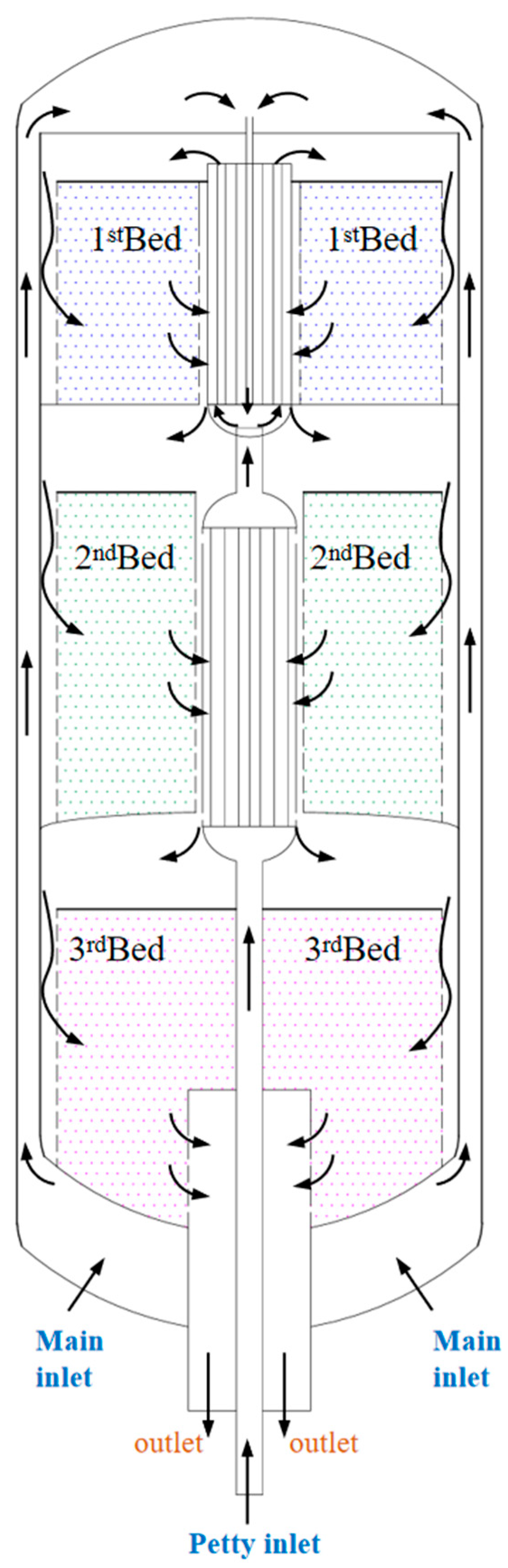
Figure 1 illustrates the schematic diagram of the ammonia synthesis reactor. The reactor feed is divided into primary (58%) and secondary (42%) streams. The primary feed enters radially from the reactor side. A smaller feed stream from the cylindrical channel at the mid-catalyst bed passes through the third bed, then flows into the second heat exchanger tubes between the second and third beds. After heat exchange with outlet gas from the second bed, the preheated stream exits the exchanger. The primary gas enters the reactor side and flows through the central tubes of the first heat exchanger. Within these tubes, heat exchange occurs between the exchanger and the secondary stream, cooling the latter. The combined feed mixture then enters the first heat exchanger tubes. Preheated by exchanging heat with outlet gas from the first bed, the feed exits the exchanger and enters the catalyst beds. A portion of the feed enters the first bed axially from the top, while the remainder flows radially into the catalyst beds through gaps between the reactor wall and the porous-bed walls. Gas traverses the beds radially and exits via the central perforated cylinder. The front 50 cm of the central cylinder and bed walls remain unperforated, enforcing axial flow in this section. All beds share identical configurations, with exceptions: the first 75 cm of the second bed and the initial 1 m of the third bed operate in axial flow. Across all three beds, gas enters axially (top) and radially (side), exiting through the central tube. After cooling in the interbed heat exchangers, gas re-enters subsequent beds. Bed lengths measure 5.7 m, 9.9 m, and 11.6 m from top to bottom.
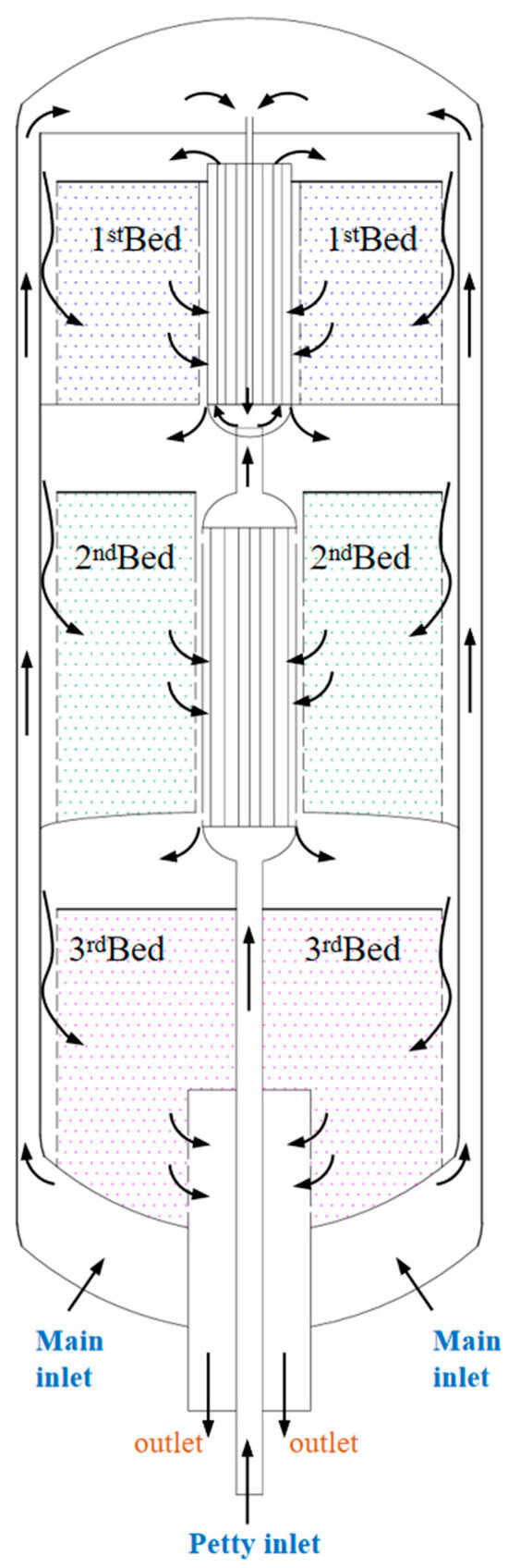
Figure 1.
Schematic diagram of the ammonia synthesis reactor.
3.2. Reactor Simplification and Modeling
Given the axial symmetry of the ammonia synthesis reactor in the two-dimensional model, the central axis is defined as the symmetry boundary, with modeling focused on the right half.
Based on the reactor prototype in Figure 1, dimensions are specified as follows: three catalyst beds with lengths of 5.7 m, 9.9 m, and 11.6 m from top to bottom, each with a width of 5.5 m on both the left and right sides. The remaining dimensions are derived from the schematic. The reactor is modeled in Design Model, comprising three regions: the top section with catalyst beds, heat exchangers with inlet piping, and the bottom section. The key dimensions are as follows.
- (1)
- Top Section and Catalyst Beds:
The two-dimensional model simplifies the original axisymmetric geometry by retaining only the right half with a symmetry axis. Total reactor height is 40 m, and width is 9 m. From top to bottom: the top dome has a diameter of 18 m; the cylindrical section spans 2 m; the elliptical section has a minor axis radius of 1 m. The three catalyst beds are positioned 0.55 m from the right-side inlet piping wall. Catalyst Bed 1 is 0.27 m from Heat Exchanger 1 on the left; Bed 2 is 0.58 m from Heat Exchanger 2; the upper half of Bed 3 is 0.5 m from the left wall, while the lower half is 2.5 m from the left wall.
- (2)
- Heat Exchangers and Inlet Piping.
The central gas inlet pipe 1 has a diameter of 0.8 m and a length of 37 m. The two lateral gas inlet pipes 2 each have a diameter of 1 m and a length of 35.3 m. The upper heat exchanger 1 has a total length of 8.5 m, featuring a semi-circular lower head (3 m diameter) and a 7 m cylindrical section. Simplified as 3 tube passes and 4 shell passes, its tube side diameter is 1 m, and shell side diameter is 0.3 m. The lower heat exchanger 2, positioned 1.5 m vertically below heat exchanger 1 and connected via inlet pipe 1, has a total length of 10 m. Both its upper and lower heads are dished (3 m diameter), with 1 m cylindrical sections at the top and bottom, and 0.5 m conical sections. Simplified as 3 tube passes and 4 shell passes, heat exchanger 1’s tube side diameter is 0.5 m (shell side: 0.3 m), while heat exchanger 2’s tube side diameter is 0.8 m (shell side: 0.3 m). The bottom of heat exchanger 2 is located 14.5 m above the reactor base.
- (3)
- Reactor Base.
Inlet pipes 1 and 2 extend 1 m outward. Pipe 2 inlet is vertically 1.7 m higher than Pipe 1 inlet. The reactor base features an arc curvature radius of 24.65 m.
The constructed sketch line bodies are selected from the completed sketch. After creating the sketch line bodies, enclosed curves are chosen to generate edge surfaces for each enclosed area. The entire model is then partitioned into five independent regions using Boolean operations tools, comprising two fluid domains and three porous media regions. Each region is subsequently named.
Given the reactor’s intricate internal structure and the non-uniform reactions within the catalyst beds, this partial heterogeneity marginally impacts the overall reaction efficacy but notably extends the iteration computation time. Hence, the study simplifies the reactor’s physical model for numerical simulations, adopting the following assumptions:
- (1)
- In the simulation calculation, the green ammonia synthesis process is regarded as a steady state process, and the operating parameters of the reactor, such as pressure, temperature and flow rate will remain constant.
- (2)
- The model regards N2 and H2 as an ideal gas mixture under high temperature and pressure. The mixing law follows the equation of state of an ideal gas, and the mass diffusion follows the molecular kinetic theory.
- (3)
- The catalyst has constant porosity and bed symmetry; it is assumed that there is no temperature and concentration gradient in the catalyst particle, and the catalyst region is regarded as a continuous porous medium.
3.3. FLUENT Simulation Setup
This study employs Fluent 16.5 for numerical simulations. The SIMPLE algorithm is utilized for equation solving, with Rhie–Chow—distance-based flux type, least squares cell based gradient handling, and second-order upwind discretization for other terms. Relaxation factors are reduced to ensure computational convergence. SIMPLE algorithm using pressure–velocity coupling (Semi-Implicit Method for Pressure-Linked Equations), achieves flow field convergence by iteratively solving the momentum and continuity equations.
In Fluent, configurations are applied to four modules: grid, definitions, boundary conditions, and solver. The specific settings are as follows.
(1) Grid: use mesh in workbench for meshing. Mesh delineation related settings: use adaptive resizing in the resizing settings with a resolution of 7 levels. The transition is slow, the span corner center is fine, and the rest remain default. The mesh quality settings change the Smooth option to High, and leave the rest as default. The insert method settings use the all triangles method, for geometry select all 5 geometries, the method is triangles, and check global settings. Finally, the Insert Encryption settings set the mesh encryption level to 3. The final total of 63,776 grid cells are divided with a mass of 0.67.
(2) Define.
General: Grid settings remain default. The solver uses a pressure-based segregated algorithm to solve the momentum equation, pressure correction equation, and component equation in sequence. The velocity field uses an absolute coordinate system format to accurately capture the Coriolis force effect of high-speed rotating fluids, which is critical in radial–axial reactors. The model settings: enable energy equation; select standard k-ε turbulence model (k represents turbulent kinetic energy, ε represents dissipation rate), by solving the two-equation closed Reynolds-averaged N-S equation system, which is applicable to fully developed industrial turbulence; retain defaults for other terms. Species settings: activate species transport; enable volumetric reactions in the reaction panel; default options for diffusion energy source terms; import ChemKin mechanism; use CHEMKIN-CFD solver for chemical reactions; set number of volumetric reactive species to 3; retain other defaults. Physical models: operating pressure and temperature are averaged from literature data on three-catalyst-bed operations, calculated as 160 bar and 700 K. Material settings: solid material uses “steel” exported from the Fluent database; mixture material is nitrogen–hydrogen–ammonia gas blend identified by the ChemKin mechanism. Cell zone conditions: fluid domains face1 and face2 retain defaults; porous media regions (porousmedia1, porousmedia2, porousmedia3) use default directional vectors. Based on reference [38], parameters for iron-based ammonia synthesis catalyst include porosity 0.3693, average particle diameter 4.45 mm, specific surface area 13.34 m2/g, bulk density 2.36 g/cm3. Inertial resistance and viscous resistance are derived from the porosity using the following formulas.
Inertia resistance:
Penetration rate:
Viscous resistance is equal to the reciprocal of permeability:
Post-calculation with input data yields inertial resistance of 9849 m−1, penetration rate: of 1.67 × 10⁻⁸ m2, and viscous resistance of 59,824,486 m−2. The catalyst in the beds exhibits isotropic properties with identical parameters in the x and y directions. Other settings retain defaults. Reaction options are checked, mechanism defaults retained; surface-to-volume ratio is calculated as 31,482,400 m−1 by multiplying the specific surface area with the bulk density.
(3) Boundary conditions.
In the boundary condition setup, configure the physical properties for walls, axis, gas inlets, and gas outlet. For walls: momentum settings retain defaults; thermal settings are modified to fixed temperature 700 K; wall material is steel with properties—density 8030 kg/m3, specific heat Cp = 502.48 J/(kg·K), thermal conductivity 16.27 W/(m·K). Outlet is set as pressure-outlet with all other options default. Axis “axis” type set to symmetry; interface and internal face settings retain defaults. Both gas inlets are configured as velocity-inlets, with molar flow rates 39,239 mol/h—calculated as v_inlet1 = 0.1553 m/s and v_inlet2 = 0.05085 m/s. Initialization parameters: gauge pressure 15,000,000 Pa, temperature 350 K; species options select component mole fractions—hydrogen 0.75, nitrogen 0.25. The CFD simulations strictly employed the Peng–Robinson real gas equation of state throughout all calculations at 15 MPa.
(4) Solve.
Set the algorithm to SIMPLE, enable the gas-phase energy equations for N2, H2, NH3, set all discretization schemes to second-order upwind, initialize parameters, define calculation steps, and start computation until convergence.
After completing the initial simulation, adjust the total gas flow rates at both inlets to 19,619.5 mol/h, 35,315.1 mol/h, 43,162.9 mol/h, 58,859.5 mol/h, 78,478 mol/h, 117,717 mol/h, 196,195 mol/h, and 313,912 mol/h (corresponding to 50%, 90%, 110%, 150%, 200%, 300%, 500%, and 800% of the baseline flow rate 39,239 mol/h). Retain all the other settings unchanged to perform the multiple simulations and collect the results.
3.4. Training Strategies and Multitasking Optimization
- (1)
- Data preparation.
Nd = 104 spatial points covering the flow, temperature, and component concentration fields were sampled from the Fluent steady-state simulation results as a supervised dataset. The boundary point Nb = 500 consists of inlet, outlet, and wall coordinates.
- (2)
- Adaptive weight adjustment.
A dynamic weight assignment strategy based on residual variance is adopted [39], where is set initially and the weights are adjusted according to the relative size of each loss term after every 1000 iterations to avoid gradient flooding.
- (3)
- Training process.
The Adam optimizer is used for initial training (learning rate 10−3), followed by switching to the L-BFGS optimizer to accelerate convergence. To enhance the ability to capture the reaction kinetics, encrypted sampling points in the catalyst bed region are prioritized.
4. Simulation Results and Analysis
4.1. CFD Simulation Accuracy Verification
As shown in Table 3, To verify grid independence and monitor changes in ammonia concentration at the outlet. When the number of grids increases to 128,935 (Fine level), the concentration change is <1.5%, indicating that 63,776 grids (Base level) have converged. Subsequent analyses are based on this optimized grid.
Table 3.
Grid sensitivity study.
For the green ammonia synthesis reactor set up with the same feed as the industrial data (containing N2: 0.2219, H2: 0.6703, CH4: 0.0542, Ar: 0.0256, ammonia: 0.0276), the results of the exit bed were verified with the CFD simulation, and the comparison between the model results and the industrial data is shown in Table 4. The simulation results are in good agreement with the industrial data in terms of bed temperature, with the maximum relative error within 2.9%. The maximum relative error in the molar fraction of ammonia is within 10%, so the model is accurate and reliable in predicting the flow field changes after changing the operating conditions of the reactor.
Table 4.
Comparison of experimental data and simulation results of the ammonia synthesis reactor.
4.2. Flow Field Distribution
From the flow field diagram in Figure 2a, it can be seen that at the middle secondary inlet, the compressed gas mixture enters the reactor at 0.1553 m/s due to the increasing temperature and gas expansion. The velocity increases slightly at first, and enters the first heat exchanger where due to the increasing diameter of the tube the velocity decreases at first, and then increases due to the increasing temperature. After entering the second heat exchanger, the gas merges with the main inlet pipe and the velocity increases further before entering the reaction region. In the reaction region, according to the trace diagram, the heated gas mixture can enter the porous media region from both axial and radial directions for reaction in the first and second reaction beds where the gas enters mainly from the axial direction. In the third reaction bed the gas enters mainly from the radial direction, and outputs from the radial direction to the outlet position. Figure 2b shows the trace diagram of fluid particles at different production loads. Influenced by the rotating airflow, the fluid particles generally rotate within the catalyst bed. The residence time of the fluid particles lengthens with decreasing load and the trajectories of the fluid particles become denser, a change that could accelerate the adsorption and diffusion processes on the catalyst surface and create more active sites for the reaction. Moreover, the radial flow pattern, characterized by gas entering from the periphery and converging towards the center, inherently promotes a more uniform distribution of flow and reactants across the catalyst bed cross-section. This uniformity contributes significantly to the reactor’s operational stability by mitigating the localized impacts of feed flow variations.
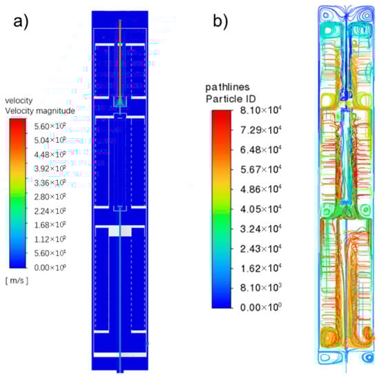
Figure 2.
Velocity field distribution in ammonia synthesis reactor. (a) Velocity distribution; (b) flow field traces.
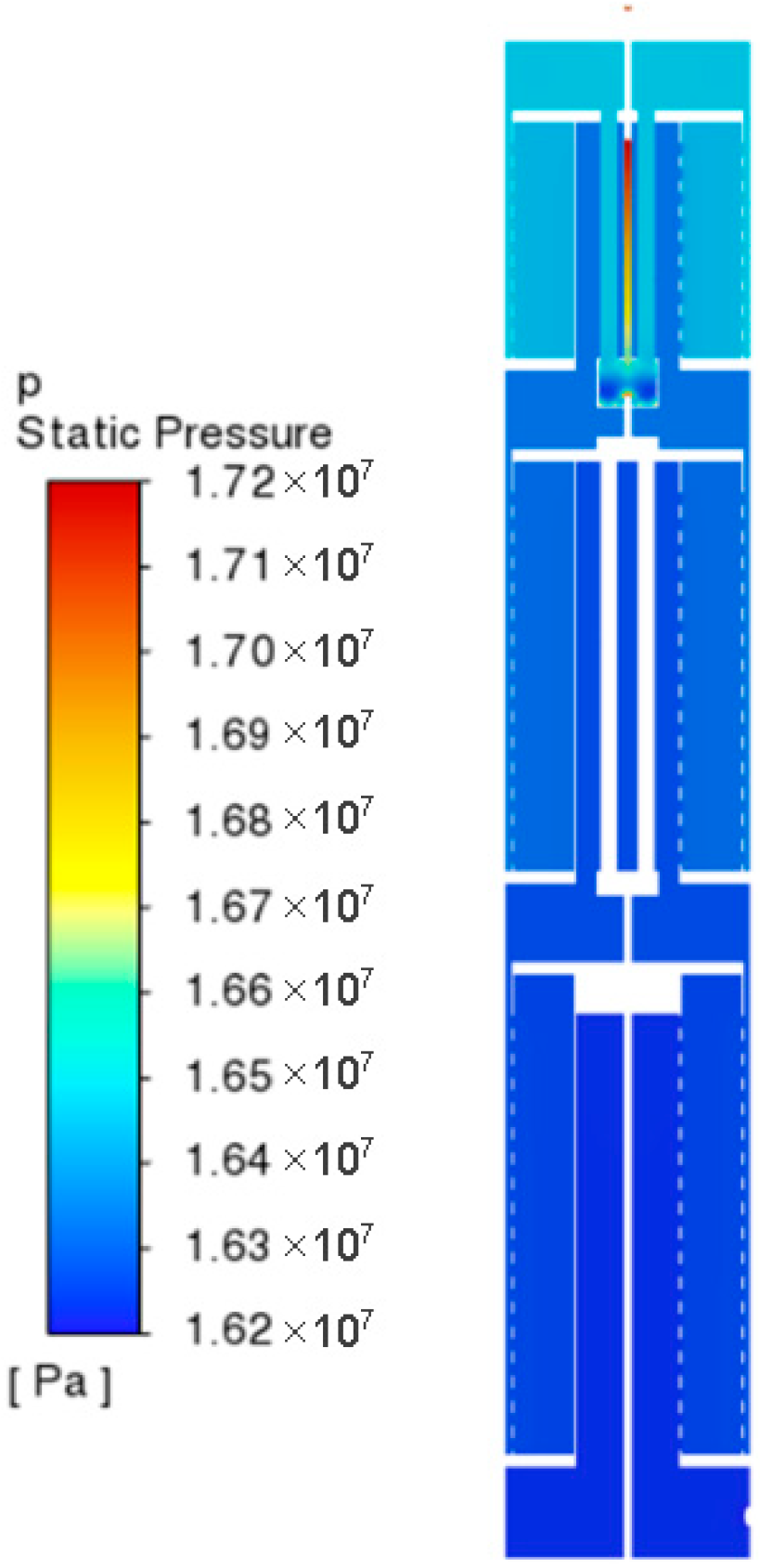
Figure 3 represents the overall pressure distribution of the ammonia synthesis reactor; this paper discusses the static pressure of the reactor as whether the pressure is uniformly distributed can directly affect the reaction process of the whole system. As can be seen from the figure, The pressure in the three catalyst beds remains uniform in the radial direction, while along the flow direction (the first to the third beds) it shows a stepwise slight decreasing trend. The reason is that the two feeds are mixed in one place in the mixing chamber and the pressure reaches a peak, and then the mixed gases flow into the three catalyst beds sequentially through the gas distributor. The fluids are continuously diverted from the openings of the distributor to make the hydrostatic pressure decrease, so the pressure remains stable in the radial direction of the catalyst beds, and the pressure along the direction of the fluid flow is also only in a slightly reduced state.

Figure 3.
Pressure distribution of ammonia synthesis reactor.
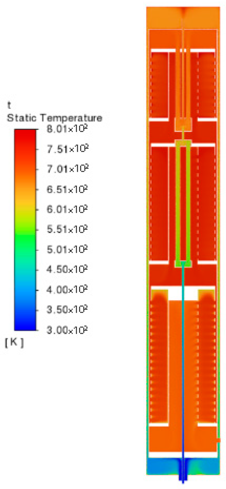
Due to the exothermic nature of the ammonia synthesis reaction and the optimal catalytic activity of the iron-based catalyst at approximately 700 K, the catalyst beds maintain a near-uniform temperature of 700 K with localized fluctuations of less than ±15 K. The feed gas mixture is rapidly preheated to the target reaction temperature before entering the catalyst beds via heat exchange with the hot product stream. At the gas outlet, the temperature decreases to 650–680 K due to heat dissipation to the ambient environment through the reactor walls.
Figure 4 reflects the temperature distribution of the reactor temperature in the region between 695–710 K. It can be seen that the vast majority of the region in the reactor is in this temperature range, the low temperature region within the temperature range is mainly concentrated in the reactor gas outlet, the gas heating section, as well as the fluid region near the heat exchanger in the reaction region. It is obvious that the gas in the reaction area is also involved in the heating of the feed gas. The high temperature region in this temperature range is mainly in the three catalyst beds, due to the exothermic reaction of the ammonia synthesis reaction. The heat released from the reaction will make the temperature of the nearby area rise. The most intense reaction will occur at the top of catalyst bed 1 when the material just enters the reaction area, so the top of catalyst bed 1 has the highest temperature. After that, the reaction will occur at the top of catalyst bed 2, which is a little inferior to that at the top of bed 1. The temperature inside the three catalyst beds is higher due to the progress of the reaction, and the reaction is more intense than that at the top of bed 1. The temperature inside the catalyst beds is significantly higher than the rest of the reactor due to the reaction.

Figure 4.
Temperature distribution of the ammonia synthesis reactor.
The distribution of the reaction product ammonia gas inside the reactor is reflected in Figure 5. In the green ammonia reactor, the feed gas enters the three catalyst beds sequentially, and the ammonia concentration increases in the axial direction of the reactor. Inside each catalyst bed, the gas enters radially from the periphery of the bed and reacts as it flows towards the central outlet duct. The combined effect of the high radial flow velocity and the relatively homogeneous catalyst packing leads to a largely uniform radial distribution of the ammonia mole fraction within each individual catalyst bed. The primary increase in ammonia concentration occurs along the axial direction as the gas sequentially passes through the three catalyst beds, resulting in a step-wise increase in concentration from Bed 1 to Bed 3. Axial variations within a single bed are minimal due to the dominant radial flow component. This behavior is attributed to the reactor design featuring closed bed tops and annular gas distributors that ensure high radial flow velocities compared to the axial component.
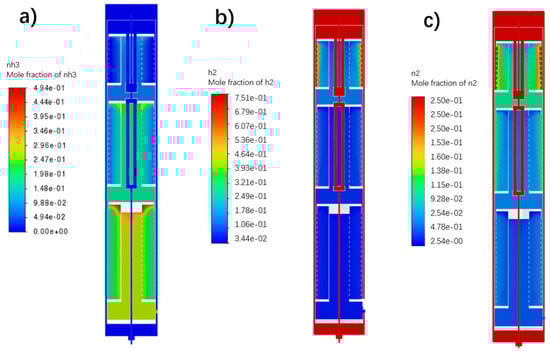
Figure 5.
Distribution of molar fraction of ammonia gas in ammonia synthesis reactor. (a) Mole fraction of NH3; (b) Mole fraction of H2; (c) Mole fraction of N2.
4.3. Validation and Efficiency Analysis of PINN-Assisted Modeling
To validate the effectiveness of the physical information neural network (PINN) in modeling green ammonia reactors, this study trains a PINN model based on steady-state flow field data generated by Fluent with an inlet gas of 39,239 mol/h and compares the consistency of its prediction results with CFD simulations, while evaluating its computational efficiency advantage under dynamic operating conditions.
- (1)
- Accuracy of flow field and component distribution prediction.
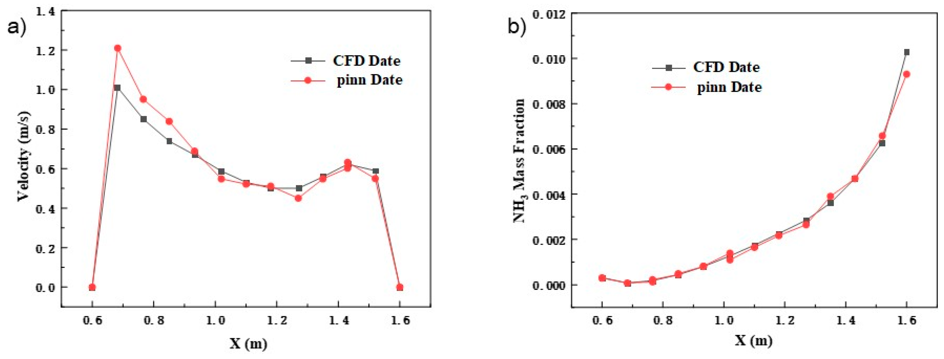
Figure 6 and Table 5 systematically verify the reliability of the PINN method in modeling the complex reaction flow field by comparing the results of axial velocity and ammonia molar fraction distribution in the catalyst bed 1 region between PINN and CFD. In terms of axial velocity distribution, PINN not only accurately reproduces the spatial distribution characteristics of the high velocity zone at the top 0.6–0.8 m and the low velocity zone at the bottom 1.4–1.6 m in the CFD simulation, but also achieves an overall prediction accuracy of 96.8%, with the maximum relative error only in the local area within 0.2 m near the wall, with a value of 4.5%—this fully satisfies the requirements of engineering applications. In terms of ammonia molar fraction prediction, the PINN simulation of the core reaction zone in the middle of the bed from 2.0–3.0 m is particularly accurate, with an average error of less than 2.8%, which accurately captures the gradient change of ammonia concentration in this zone from 45% to 78%. Notably, in the near-wall region, the prediction error rises to 6.1% due to the significant boundary layer effect and the insufficient sampling density of the training data, which mainly stems from the drastic changes in the physical field caused by the large velocity gradient at the wall and the complex reaction boundary conditions. Through further analysis, it is found that the errors in these regions are mainly concentrated near the axial position of 1.2 m to 1.4 m, which corresponds exactly to the location of the flow perturbation caused by local structures such as the support members in the catalyst bed. This phenomenon suggests that the introduction of a residual-based adaptive sampling strategy in the subsequent work, focusing on encrypting the training data points in the high-gradient regions, is expected to further reduce the overall prediction error to less than 5%, and thus enhance the applicability of PINN in the full-scale modeling of industrial reactors. Although elevated errors (∼8.7%) are observed in near-wall regions with steep velocity gradients, this stems from the trade-off between computational efficiency and local resolution. Uniform sampling was prioritized to maintain real-time prediction capability for reactor-scale dynamics. Notably, the global accuracy remains within acceptable bounds for engineering design—catalyst bed temperature deviations average 3.3% and ammonia concentration errors are below 2.8% across all scenarios, demonstrating robust performance despite localized limitations.
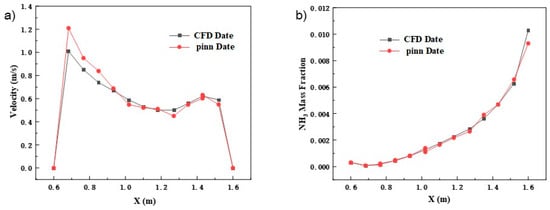
Figure 6.
Comparison of PINN and CFD axial distribution results. (a) Comparison of axial velocity distribution; (b) comparison of ammonia mole fraction distribution.
Table 5.
Comparison of PINN and CFD prediction accuracy.
In addition, the comparison results also show that the ability of PINN to capture the reaction-flow coupling features in the mainstream region is comparable to that of CFD, but it has a significant advantage in computational efficiency, with a single prediction time consuming only 1/200 of that of CFD, which provides a new technological path for real-time optimization and control of reactors. Although PINN achieves 200× acceleration during the inference phase, its upfront training cost is significantly higher than a single CFD calculation (4.5 h vs. 240 s). Therefore, its core value lies in scenarios requiring iterative iterations, such as dynamic operating condition optimization and parameter sensitivity analysis, where PINN can quickly respond to changing conditions. Especially in scenarios with fluctuating hydrogen flow rates, PINN can complete 100 parameter optimization schemes within 10 min, while CFD requires 6.7 h—this timeliness is critical for real-time control under the fluctuating conditions of renewable energy.
PINN ensures prediction reliability through physical equation residual loss, while CFD data only provides weak supervision. In areas without data (such as the center of the bed), physical constraints dominate the prediction results, with flow velocity distribution errors still <6.5%, proving that physical mechanisms are the cornerstone of accuracy, while CFD data only assists in local calibration.
- (2)
- Parameter inversion and uncertainty quantification.
Based on the embedding properties of differential equations of PINN, the inverse ability of the reaction kinetic parameters was further explored in this study. Using the test data of ammonia concentration at the outlet of catalyst bed 3, the reaction kinetics were jointly optimized by PINN in terms of the pre-factor k0 and activation energy Ea. The comparison between the optimized parameters and the actual values is shown in Table 6, and the results show that the relative error of the inversion value of the PINN is less than 7%, which not only verifies the high-precision parameter identification ability of the PINN in the strong nonlinear reaction-flow coupling problem, but also reveals its unique advantage of effectively compensating the data sparsity through physical constraints. This can be used for the green ammonia reactor under fluctuating operating conditions. This result not only verifies the high-accuracy parameter identification ability of PINN in the strong nonlinear reaction-flow coupling problem, but also reveals its unique advantage of effectively compensating data sparsity through physical constraints, which provides a reliable theoretical tool for the real-time parameter calibration and adaptive control of the green ammonia reactor under fluctuating conditions.
Table 6.
Comparison of reaction rate constant inversion results.
4.4. Analysis of the Effect of Ammonia Export Content and Intake Volume
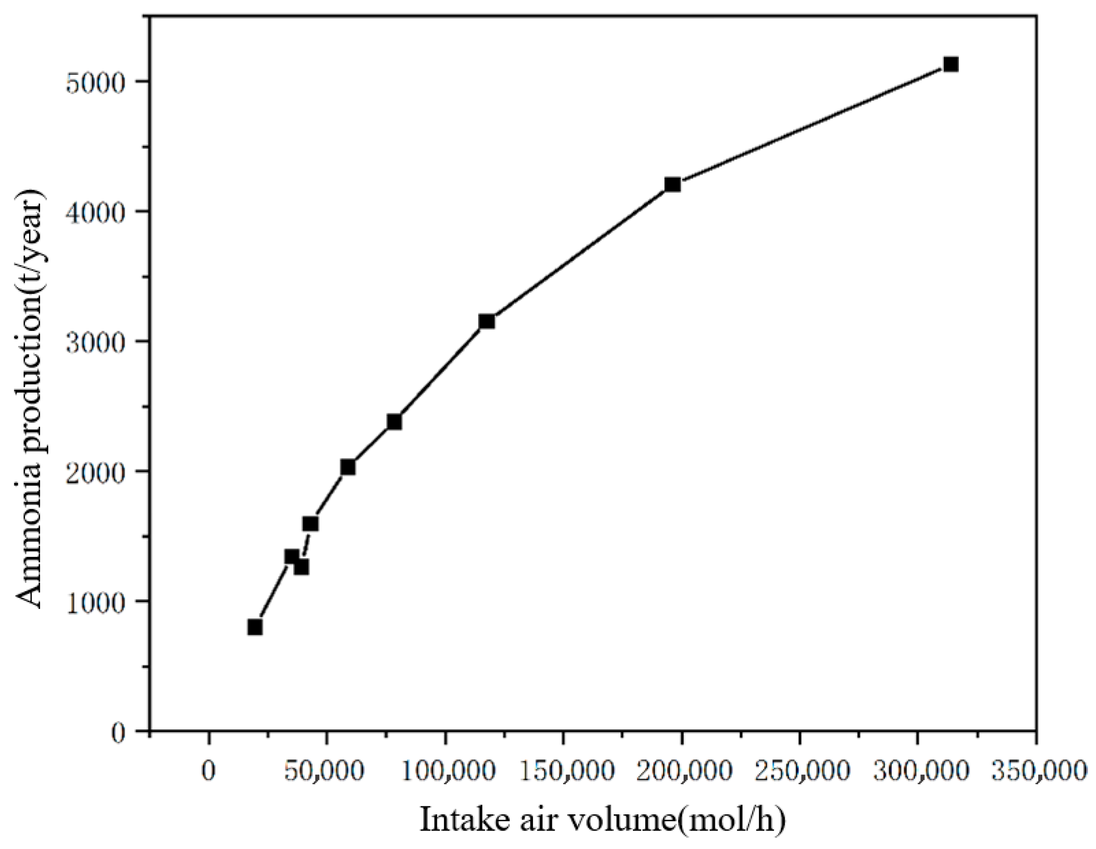
Assuming that the reactor produces 24 h a day without interruption and 300 days a year, the annual production of ammonia at this inlet volume can be calculated as below based on the inlet volume and the corresponding ammonia conversion rate.
From Figure 7, it can be concluded that the overall ammonia production is positively correlated with the inlet volume, but the growth rate of ammonia production decreases with the increase of the inlet volume: The appropriate inlet volume should be selected in industrial production after comprehensive consideration of the ammonia conversion rate and the production volume, which not only ensures sufficient production, but also reduces the wastage and lowers the cost of gas separation and recycling. When the feed gas volume is 39,239 mol/h, the annual output is 1264 tons, which achieves the annual ammonia output required in the design.
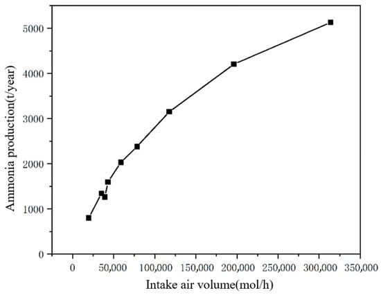
Figure 7.
Annual ammonia production versus gas intake.
5. Conclusions
Through the CFD simulation analysis and PINN-assisted modeling study of the ammonia synthesis reactor, the multi-scale coupling mechanism between flow, heat transfer, and reaction process is systematically revealed. The study shows that the flow field in the reactor is characterized by an obvious axial–radial synergistic distribution, and the axial flow velocity in the inlet section increases continuously due to thermal acceleration, while the flow in the catalyst bed tends to be stable, forming a typical distribution pattern of “fast in the middle and slow on both sides”. Pressure field analysis showed that the pressure in the non-reaction zone increased axially, while the pressure in the reaction zone showed a trend of decreasing and then increasing, while the high-pressure zone was mainly concentrated at the top and bottom of the tower. The distribution of the temperature field showed that the temperature in the reaction zone was maintained at the optimal catalytic activity range of 695–710 K, in which the catalyst bed was the obvious high temperature zone, and the temperatures around the heat exchanger and the exit area were relatively low due to the heat exchange effect.
In particular, by introducing the physical information neural network (PINN) to assist the modeling, the CFD–PINN coupling framework proposed in this study was validated for its inherent consistency through a cross-validation mechanism. The deviation between traditional CFD simulation results and key parameters of industrial benchmark data is less than 3.2%, while PINN maintains a prediction error of less than 5.5% in physically dominant regions (such as the core region of the catalyst bed) without CFD data supervision. This two-way mutual verification relationship confirms the robustness of this method in renewable energy fluctuation scenarios. At the same time, PINN successfully realized the efficient inversion of reaction kinetics parameters, with the inversion errors of the prefactor k0 and the activation energy Ea being both lower than 7%. These results fully confirm that PINN can effectively integrate experimental data and numerical simulation results under the premise of retaining the physical laws, which provides a new research idea for reactor performance optimization.
This study lays an important foundation for the development of an intelligent regulation system adapted to the fluctuating characteristics of renewable energy sources. In the future, we can realize the whole process of reactor upgrading from offline design to on-line optimization by constructing a hybrid PINN–CFD solver, which can promote green ammonia production in the direction of high efficiency and intelligence. While the model exhibits slight accuracy degradation in high-shear regions, this does not impact core reactor performance metrics. The unified resolution strategy remains justified for system-level dynamic analysis under hydrogen supply fluctuations.
Author Contributions
Conceptualization, G.H. and X.Z.; methodology, R.X. and S.Z.; software, Y.W.; validation, F.R., X.J. and W.F.; formal analysis, L.Z.; data curation, X.Z.; writing—original draft preparation, R.X.; writing—review and editing, G.H.; visualization, Y.W.; project administration, X.J.; funding acquisition, X.J. All authors have read and agreed to the published version of the manuscript.
Funding
This research was funded by the National Key Research and Development Program of China grant number 2021YFB40005 And the APC was funded by G.H. and X.J.
Data Availability Statement
The data presented in this study are available on request from the corresponding author.
Conflicts of Interest
This research was conducted in the absence of any commercial or financial relationships that could be construed as a potential conflict of interest. Authors Mrs. Ran Xu, Mr. Shibin Zhang and Mr. Fengwei Rong were employed by CNNP Rich Energy Corporation Limited. The remaining authors declare that the research was conducted in the absence of any commercial or financial relationships that could be construed as a potential conflict of interest.
Abbreviations
A list of symbols:
| Symbol | Meaning |
| A | Inertial resistance coefficient, kg·m−4 |
| av | Specific surface area of catalyst, - |
| B | Viscous resistance coefficient, kg·m−5·s−1 |
| C1 | Viscous resistance coefficient (Ergun eq.), m−2 |
| C2 | Inertial resistance coefficient (Ergun eq.), m−1 |
| Cj | Molar concentration of species j, mol·m−3 |
| Cp | Specific heat capacity, J·kg−1·K−1 |
| CFD | Computational fluid dynamics |
| PINNs | Physics-informed neural networks |
| dp | Catalyst particle diameter, mm |
| Ea | Activation energy, kJ·mol−1 |
| f | Friction factor (Tallmadge eq.), - |
| Gf | Gibbs free energy of formation, J·mol−1 |
| H | Enthalpy change, J·mol−1 |
| hf | Heat transfer coefficient, W·m−2·K−1 |
| Kf | Fugacity-based equilibrium constant, - |
| Kp | Pressure-based equilibrium constant, Pa−2 |
| k | Thermal conductivity, W·m−1·K−1 |
| Re | Reynolds number, - |
| r | Radial coordinate/Reaction rate, m/mol·m−3·s−1 |
| Si | Source term for species i, kg·m−3·s−1 |
| Sh | Energy source term, W·m−3 |
| T | Temperature, K |
| t | Time, s |
| u | Velocity vector, m·s−1 |
| ur, uz | Radial/axial velocity components, m·s−1 |
| Yi | Mass fraction of species i, - |
| ε | Porosity |
| η | Catalyst effectiveness factor |
References
- Yan, X.; Zheng, W.; Wei, Y.; Yan, Z. Current Status and Economic Analysis of Green Hydrogen Energy Industry Chain. Processes 2024, 12, 315. [Google Scholar] [CrossRef]
- Li, J.; Lin, J.; Song, Y. Capacity Optimization of Hydrogen Buffer Tanks in Renewable Power to Ammonia (P2A) System. In Proceedings of the 2020 IEEE Power & Energy Society General Meeting (PESGM), Montreal, QC, Canada, 2–6 August 2020; pp. 1–5. [Google Scholar]
- Deng, W.; Huang, C.; Li, X.; Zhang, H.; Dai, Y. Dynamic Simulation Analysis and Optimization of Green Ammonia Production Process under Transition State. Processes 2022, 10, 2143. [Google Scholar] [CrossRef]
- Zhang, Q.; Peng, J.; Jiang, S.; Xiong, H.; Fu, X.; Shang, S.; Xu, J.; He, G.; Chen, P.-C. Plasma-activated 2D CuMnO2 nanosheet catalysts with rich oxygen vacancies for efficient CO2 electroreduction. Appl. Catal. B Environ. Energy 2025, 371, 125255. [Google Scholar] [CrossRef]
- Qi, M.; Kim, M.; Dat Vo, N.; Yin, L.; Liu, Y.; Park, J.; Moon, I. Proposal and surrogate-based cost-optimal design of an innovative green ammonia and electricity co-production system via liquid air energy storage. Appl. Energy 2022, 314, 118965. [Google Scholar] [CrossRef]
- Wang, L.; Xia, M.; Wang, H.; Huang, K.; Qian, C.; Maravelias, C.T.; Ozin, G.A. Greening Ammonia toward the Solar Ammonia Refinery. Joule 2018, 2, 1055–1074. [Google Scholar] [CrossRef]
- Wu, B. Integration of mixing, heat transfer, and biochemical reaction kinetics in anaerobic methane fermentation. Biotechnol. Bioeng. 2012, 109, 2864–2874. [Google Scholar] [CrossRef]
- He, G.; Dang, Y.; Zhou, L.; Dai, Y.; Que, Y.; Ji, X. Architecture model proposal of innovative intelligent manufacturing in the chemical industry based on multi-scale integration and key technologies. Comput. Chem. Eng. 2020, 141, 106967. [Google Scholar] [CrossRef]
- Cha, J.; Park, Y.; Brigljević, B.; Lee, B.; Lim, D.; Lee, T.; Jeong, H.; Kim, Y.; Sohn, H.; Mikulčić, H.; et al. An efficient process for sustainable and scalable hydrogen production from green ammonia. Renew. Sustain. Energy Rev. 2021, 152, 111562. [Google Scholar] [CrossRef]
- Meier, A.; Ganz, J.; Steinfeld, A. Modeling of a novel high-temperature solar chemical reactor. Chem. Eng. Sci. 1996, 51, 3181–3186. [Google Scholar] [CrossRef]
- Dashti, A.; Khorsand, K.; Ahmadi Marvast, M.; Kakavand, M. Modeling and simulation of ammonia synthesis reactor. Pet. Coal 2006, 48, 15–23. [Google Scholar]
- Khademi, M.H.; Sabbaghi, R.S. Comparison between three types of ammonia synthesis reactor configurations in terms of cooling methods. Chem. Eng. Res. Des. 2017, 128, 306–317. [Google Scholar] [CrossRef]
- Elnashaie, S.S.E.H.; Mahfouz, A.T.; Elshishini, S.S. Digital simulation of an industrial ammonia reactor. Chem. Eng. Process. Process Intensif. 1988, 23, 165–177. [Google Scholar] [CrossRef]
- Baddour, R.F.; Brian, P.L.T.; Logeais, B.A.; Eymery, J.P. Steady-state simulation of an ammonia synthesis converter. Chem. Eng. Sci. 1965, 20, 281–292. [Google Scholar] [CrossRef]
- Gaines, L.D. Ammonia synthesis loop variables investigated by steady-state simulation. Chem. Eng. Sci. 1979, 34, 37–50. [Google Scholar] [CrossRef]
- Panahandeh, M.R.; Fathikaljahi, J.; Taheri, M. Steady-State Modeling and Simulation of an Axial-Radial Ammonia Synthesis Reactor. Chem. Eng. Technol. 2003, 26, 666–671. [Google Scholar] [CrossRef]
- Zardi, F.; Bonvin, D. Modeling, simulation and model validation for an axial-radial ammonia synthesis reactor. Chem. Eng. Sci. 1992, 47, 2523–2528. [Google Scholar] [CrossRef]
- Azarhoosh, M.J.; Farivar, F.; Ale Ebrahim, H. Simulation and optimization of a horizontal ammonia synthesis reactor using genetic algorithm. RSC Adv. 2014, 4, 13419–13429. [Google Scholar] [CrossRef]
- Flowers, D.; Aceves, S.; Westbrook, C.K.; Smith, J.R.; Dibble, R. Detailed Chemical Kinetic Simulation of Natural Gas HCCI Combustion: Gas Composition Effects and Investigation of Control Strategies. J. Eng. Gas Turbines Power 2000, 123, 433–439. [Google Scholar] [CrossRef]
- Bahri, P.A.; Bandoni, J.A.; Romagnoli, J.A. Effect of disturbances in optimizing control: Steady-state open-loop backoff problem. AIChE J. 1996, 42, 983–994. [Google Scholar] [CrossRef]
- Yasar, O.; Rutland, C.J. Parallelization of KIVA-II on the iPSC/860 supercomputer. In Proceedings of the Conference on Parallel Computational Fluid Dynamics ‘92: Implementations and Results Using Parallel Computers: Implementations and Results Using Parallel Computers, New Brunswick, NJ, USA, 18–20 May 1992; pp. 419–425. [Google Scholar]
- Read, N.K.; Zhang, S.X.; Ray, W.H. Simulations of a LDPE reactor using computational fluid dynamics. AIChE J. 1997, 43, 104–117. [Google Scholar] [CrossRef]
- Zhang, X.; Li, G.; Zhou, Z.; Nie, L.; Dai, Y.; Ji, X.; He, G. How to Achieve Flexible Green Ammonia Production: Insights via Three-Dimensional Computational Fluid Dynamics Simulation. Ind. Eng. Chem. Res. 2024, 63, 12547–12560. [Google Scholar] [CrossRef]
- Jalili, D.; Jadidi, M.; Keshmiri, A.; Chakraborty, B.; Georgoulas, A.; Mahmoudi, Y. Transfer learning through physics-informed neural networks for bubble growth in superheated liquid domains. Int. J. Heat Mass Transf. 2024, 232, 125940. [Google Scholar] [CrossRef]
- Haghighat, E.; Raissi, M.; Moure, A.; Gomez, H.; Juanes, R. A physics-informed deep learning framework for inversion and surrogate modeling in solid mechanics. Comput. Methods Appl. Mech. Eng. 2021, 379, 113741. [Google Scholar] [CrossRef]
- Shukla, K.; Zou, Z.; Chan, C.H.; Pandey, A.; Wang, Z.; Karniadakis, G.E. NeuroSEM: A hybrid framework for simulating multiphysics problems by coupling PINNs and spectral elements. Comput. Methods Appl. Mech. Eng. 2025, 433, 117498. [Google Scholar] [CrossRef]
- Xie, M.; Zhao, X.; Zhao, D.; Fu, J.; Shelton, C.; Semlitsch, B. Predicting bifurcation and amplitude death characteristics of thermoacoustic instabilities from PINNs-derived van der Pol oscillators. J. Fluid Mech. 2024, 998, A46. [Google Scholar] [CrossRef]
- Aliakbari, M. Physics Informed Neural Networks to Solve Forward and Inverse Fluid Flow and Heat Transfer Problems. Ph.D. Thesis, Northern Arizona University, Flagstaff, AZ, USA, 2023. [Google Scholar]
- Yang, Y.; Yang, Q.; Deng, Y.; He, Q. Moving sampling physics-informed neural networks induced by moving mesh PDE. Neural Netw. 2024, 180, 106706. [Google Scholar] [CrossRef]
- Kandemir, T.; Schuster, M.E.; Senyshyn, A.; Behrens, M.; Schlögl, R. The Haber-Bosch process revisited: On the real structure and stability of “ammonia iron” under working conditions. Angew. Chem. Int. Ed. Engl. 2013, 52, 12723–12726. [Google Scholar] [CrossRef] [PubMed]
- Kyriakou, V.; Garagounis, I.; Vourros, A.; Vasileiou, E.; Stoukides, M. An Electrochemical Haber-Bosch Process. Joule 2020, 4, 142–158. [Google Scholar] [CrossRef]
- Zhao, X.; Jia, X.; Zhang, H.; Zhou, X.; Chen, X.; Wang, H.; Hu, X.; Xu, J.; Zhou, Y.; Zhang, H.; et al. Atom-dispersed copper and nano-palladium in the boron-carbon-nitrogen matric cooperate to realize the efficient purification of nitrate wastewater and the electrochemical synthesis of ammonia. J. Hazard. Mater. 2022, 434, 128909. [Google Scholar] [CrossRef]
- Hao, D.; Wei, Y.; Mao, L.; Bai, X.; Liu, Y.; Xu, B.; Wei, W.; Ni, B.-J. Boosted selective catalytic nitrate reduction to ammonia on carbon/bismuth/bismuth oxide photocatalysts. J. Clean. Prod. 2022, 331, 129975. [Google Scholar] [CrossRef]
- Liu, H.; Hu, Z.; Li, X.; Li, Y.; Jiang, Z. Research on the performance and application of A301 type ammonia synthesis catalyst. Ind. Catal. 1994, 2, 19–26. (In Chinese) [Google Scholar]
- Boisen, A.; Dahl, S.; Nørskov, J.K.; Christensen, C.H. Why the optimal ammonia synthesis catalyst is not the optimal ammonia decomposition catalyst. J. Catal. 2005, 230, 309–312. [Google Scholar] [CrossRef]
- Palys, M.J.; McCormick, A.; Cussler, E.L.; Daoutidis, P. Modeling and Optimal Design of Absorbent Enhanced Ammonia Synthesis. Processes 2018, 6, 91. [Google Scholar] [CrossRef]
- Wang, H.F. Fully consistent Eulerian Monte Carlo fields method for solving probability density function transport equations in turbulence modeling. Phys. Fluids 2021, 33, 015118. [Google Scholar] [CrossRef]
- Liu, H. Ammonia Synthesis Catalysts: Innovation and Practice; World Scientific Publishing: Singapore, 2013; pp. 1–872. [Google Scholar]
- Wang, L.; Xie, J. Enhancing Extreme Learning Machine Robustness via Residual-Variance-Aware Dynamic Weighting and Broyden–Fletcher–Goldfarb–Shanno Optimization: Application to Metro Crowd Flow Prediction. Systems 2025, 13, 349. [Google Scholar] [CrossRef]


Disclaimer/Publisher’s Note: The statements, opinions and data contained in all publications are solely those of the individual author(s) and contributor(s) and not of MDPI and/or the editor(s). MDPI and/or the editor(s) disclaim responsibility for any injury to people or property resulting from any ideas, methods, instructions or products referred to in the content. |
© 2025 by the authors. Licensee MDPI, Basel, Switzerland. This article is an open access article distributed under the terms and conditions of the Creative Commons Attribution (CC BY) license (https://creativecommons.org/licenses/by/4.0/).