Research on Mechanical Fault Diagnosis Method of Isolation Switch Based on Variational Autoencoder

Abstract

This study presents a Variational Autoencoder (VAE)-based framework for the unsupervised mechanical fault diagnosis of high-voltage isolation switches. By analyzing voltage and current signals to compute instantaneous power sequences, the method detects anomalies through reconstruction errors. Experimental results from both laboratory and real-world datasets demonstrate that the VAE model outperforms traditional methods, offering high diagnostic accuracy and robustness without the need for labeled data or manual feature extraction. This approach provides an effective solution for the real-time monitoring and predictive maintenance of high-voltage switchgear.

1. Introduction

High-voltage isolation switches serve critical functions in power systems by isolating power, performing switching operations, and connecting or disconnecting low-current circuits. As such, their reliability directly affects grid safety and stability [1,2,3,4]. However, due to long-term exposure to harsh environments such as wind, snow, and dust, and their typically simple, low-cost structures, these switches are highly susceptible to mechanical failures. Such failures, often caused by structural fatigue, material degradation, or design defects, can lead to unplanned outages or even system-wide blackouts. Therefore, developing accurate, real-time, and robust fault diagnosis mechanisms for isolation switches is critical for the resilience of modern power systems.

Traditional methods for fault diagnosis in high-voltage isolation switches can be broadly categorized into three groups: time-series similarity analysis, signal transformation techniques, and supervised learning approaches. Dynamic Time Warping (DTW) is a representative similarity-based method that aligns sequences of different lengths to assess similarity, but it is sensitive to noise and time shifts [5]. Signal transformation techniques, such as wavelet transforms, enable time-frequency analysis of transient features but rely heavily on the selection of appropriate wavelet bases, which may limit their generalization across varying fault types [6]. Supervised classification methods like Support Vector Machines (SVMs) have also been widely applied [7,8], offering improved accuracy over traditional rule-based systems. However, these approaches require extensive labeled data and manual feature extraction, which significantly limits their scalability and adaptability in complex field conditions. Collectively, these limitations highlight the need for more robust, generalizable, and data-efficient diagnostic frameworks.

Recent developments in deep learning have introduced new possibilities for mechanical fault diagnosis. Convolutional Neural Networks (CNNs) have demonstrated effectiveness in spatial feature extraction, while Long Short-Term Memory (LSTM) networks excel in modeling temporal dependencies. However, CNNs may overlook sequential patterns critical to mechanical behavior, and LSTMs are often computationally intensive and require extensive training data. VAEs have emerged as a promising alternative, capable of learning compact latent representations and detecting anomalies based on reconstruction errors. While some studies have employed VAEs in semi-supervised frameworks or for vibration-based diagnostics [9], few have explored their application to the power signal-based monitoring of isolation switches. Moreover, the use of unsupervised VAE models under real-world noisy and heterogeneous conditions remains limited. These gaps motivate our work to develop a VAE-based unsupervised fault diagnosis method tailored to motor power signals in high-voltage isolation switches.

Building on these challenges and the potential of VAEs, we propose an unsupervised VAE-based method for fault diagnosis in high-voltage isolation switches using motor power signals. The following tables summarize the current state of fault diagnosis research and highlight how our approach addresses existing gaps. As shown in

Table 1. Comparison of existing research and innovations.

Research Area	Methods and Techniques	Limitations	Innovations and Contributions
Fault Diagnosis	Traditional machine learning methods	Dependent on labeled data, poor adaptability	Introduces a VAE-based unsupervised learning method
Fault Type Identification	Focused on “Incomplete Close” and “Fail to Close”	Limited recognition	Uses instantaneous power signals to differentiate faults
Generalization	SVM, DTW-based traditional models	Poor performance with field data	Proposes a VAE model, showing strong generalization
Label Dependency	Requires large labeled datasets	High cost and potential inaccuracies in labeling	No need for labels; adapts to dynamic noise environments
Real-time Detection	Tested mostly in lab environments	Lack of real-world validation	Proposes a real-time fault diagnosis framework adapted to field data

and

Table 2. Fault diagnosis of high-voltage isolation switches.

Research Topic	Existing Research Results	Ongoing Challenges	Contributions of This Study
“Incomplete Close” and “Fail to Close”	Focused on mechanical fault classification	Limited recognition methods	Proposes VAE-based fault detection method
Detection Methods	Uses similarity analysis methods like DTW	Cannot adapt to different devices and environments	Proposes a VAE method, improving diagnostic accuracy
Noise Robustness	Traditional methods are vulnerable to noise	Poor robustness, difficulty handling complex environmental data	Proposes noise-robust unsupervised learning method

.

To address these gaps, this paper proposes a fully unsupervised VAE-based framework for mechanical fault detection in high-voltage isolation switches. Unlike vibration- or acoustics-based approaches, our method leverages motor power signal curves—underexplored in the current literature—to train a lightweight VAE model. The approach captures latent fault patterns directly from raw data, avoiding hand-crafted features, and allowing for real-time anomaly detection under noisy and dynamic conditions. In addition to outperforming classical methods such as DTW and wavelet transform, the model is also compared with a benchmark CNN classifier, providing a clear view of its advantages over other deep learning techniques.

Having highlighted the importance of high-voltage isolation switches and the challenges involved in fault diagnosis, we now introduce the methodology developed to address these issues and improve fault detection.

2. Methodology

Accurate data acquisition and preprocessing are critical for reliable mechanical fault diagnosis, especially in high-voltage switchgear systems.

The raw data consists of voltage and current signals collected from the driving motor of high-voltage isolation switches during switching operations, as shown in Figure 1. These signals were obtained using industrial-grade Hall effect current and voltage sensors with high linearity, mounted directly on the motor circuit to ensure minimal signal loss. The sampling frequency of 10 kHz was chosen based on engineering experience to balance signal resolution and computational cost. Data was collected from two main sources: one set from a ZF12B-126 GIS isolation switch platform in a laboratory environment and another from switches installed in an operational substation. Laboratory experiments were conducted under tightly controlled environmental conditions with a deliberate introduction of mechanical anomalies to simulate known fault types. In contrast, the field data reflect natural operational wear, component aging, temperature and humidity fluctuations, and other uncontrollable factors, thereby enriching the data with realistic variability.

Average instantaneous power was used as the key feature for fault identification, as it reflects the motor’s mechanical load characteristics [9]. Instantaneous power sequences were computed directly from the voltage and current measurements without additional filtering or preprocessing, as the industrial-grade sensors and data acquisition system provided inherently clean signals (SNR > 80 dB) with complete temporal continuity. All input sequences were normalized using z-score standardization to ensure consistent feature scaling and accelerate model convergence. This standardization retains the polarity and variation characteristics of the signals, and the asymmetry introduced by real equipment was preserved in the field data distribution. A fixed-length sliding window was used to segment the power sequences into overlapping subsequences for training, ensuring the temporal continuity of the input data.

The dataset in this study consists of two parts. The first part includes 500 samples collected from controlled experiments conducted on a ZF12B-126 high-voltage isolation switch. These experiments were designed to reflect various operating conditions, such as normal and faulty conditions of the switch operation. Due to the high repeatability of the test platform, collecting a larger number of samples would provide diminishing returns, as excessive redundancy may not contribute additional diagnostic value. Moreover, the acquisition of labeled fault data in such experiments is both time-consuming and resource intensive. The second part comprises 274 samples of field measurements obtained from an in-service substation, which captures natural variations caused by equipment aging, environmental factors, and operational uncertainties. The combination of controlled and real-world data increases the heterogeneity of the dataset, enhancing the robustness and generalization capability of the proposed fault diagnosis model.

Before selecting the Variational Autoencoder (VAE) as the core anomaly detection model, we also considered several alternative unsupervised approaches, including traditional Autoencoders (AEs), Generative Adversarial Networks (GANs), and tree-based Isolation Forests. While AEs are conceptually simpler, they often suffer from overfitting and lack a probabilistic latent representation, which limits their ability to generalize, especially in highly variable field data. Unlike traditional AEs, a VAE is able to learn the probabilistic distribution of the data, which helps it model complex, nonlinear relationships better than simple AEs.

GAN-based models, such as AnoGAN, are known for their strong generative capabilities, but they require adversarial training, which is often unstable and computationally intensive. Moreover, GANs are not specifically designed for anomaly detection, and their ability to handle noisy, real-world data is limited due to training challenges such as mode collapse. A VAE, in contrast, benefits from a more stable training process, and it directly learns the distribution of input data, making it more suitable for detecting anomalies in the context of high-voltage isolation switches, where noise and data complexity are common.

Isolation Forests, although effective for low-dimensional tabular data, are less suited for modeling temporal dependencies, especially when dealing with time-series data such as motor power signals. Isolation Forests use decision trees to isolate anomalies, but they are not designed to capture complex, sequential patterns in the data. In contrast, VAEs offer a robust probabilistic framework that models input variability and temporal dependencies more effectively, allowing for anomaly detection via reconstruction error. This makes VAEs especially well-suited to our application, which involves noisy, time-dependent power curves from motor circuits. The ability of VAEs to handle both the temporal aspect and the inherent noise in the power signals makes it a more powerful choice for this specific fault diagnosis problem.

VAE [10,11,12,13,14,15,16] is a powerful deep learning approach used to learn latent representations of input data and perform anomaly detection. It is a generative model that captures the underlying distribution of the input data by mapping it to a latent space and reconstructing it back to the original space. This section describes the VAE composition, including its encoder and decoder architecture, the reparameterization trick, and the associated loss function. Additionally, we explain how the VAE model is trained and how anomaly detection is performed based on reconstruction loss.

The model architecture consists of three main components: the encoder, the latent space, and the decoder. The encoder transforms a power sequence input x ∈ ℝ¹⁰⁰, which is extracted using the sliding window method described in Section 2, into a distribution over a latent variable z ∈ ℝ¹⁶, the latent dimensionality was empirically selected based on prior modeling experience and serves as a balance between representation capacity and overfitting risk. A reduced dimension of $z\in {ℝ}^8$ was also evaluated which yielded a comparable diagnostic performance on the current dataset. This suggests that the model is relatively insensitive to this hyperparameter under the present conditions. Yet, optimizing latent space dimensionality remains an important direction for future work, particularly when extending the framework to more diverse and heterogeneous switch data.

This is achieved using two fully connected layers with 128 and 64 neurons, respectively, each followed by ReLU activation. The encoder outputs the parameters of a Gaussian distribution, namely the mean vector μ and standard deviation vector σ.

The reparameterization trick is used to enable backpropagation through stochastic sampling. The training of the VAE minimizes a composite loss function that includes a reconstruction loss and a regularization term. The reconstruction loss is calculated as the mean squared error (MSE) between the input x and the reconstructed output $\overbrace{x}$:

$${\mathcal{L}}_{\mathcal{r}\mathcal{e}\mathcal{c}\mathcal{o}\mathcal{n}}=E_{q\left(z|x\right)}\left[|x-\widehat{x}{|}^2\right]$$

(1)

The regularization term is the Kullback–Leibler (KL) divergence between the learned posterior q(z|x) and a standard Gaussian prior, given by:

$$D_{\mathrm{KL}}(q(z|x)\Vert p(z))=-{\displaystyle \frac{1}{2}}{\displaystyle \sum _{j=1}^d\left(1+\log {\sigma }_j^2-{\mu }_j^2-{\sigma }_j^2\right)}$$

(2)

where ${\mu }_j$ is the mean of the $j$-th latent dimension; ${\sigma }_j$: standard deviation of the $j$-th latent dimension; $d$: dimensionality of latent space $z$.

The total loss function is therefore defined as:

$${\mathcal{L}}_{\mathrm{total}}={\mathcal{L}}_{\mathrm{recon}}+\beta \cdot D_{\mathrm{KL}}(q(z|x)\Vert p(z))$$

(3)

where β is a balancing coefficient, set to 1 in our implementation.

The model is trained with a learning rate of 0.001, a batch size of 64, and over 200 epochs. All input sequences are normalized using z-score standardization. Training is performed on the combined dataset described in Section 2, and validation loss is monitored to prevent overfitting.

For anomaly detection, we compute the reconstruction error for each test input. Samples whose reconstruction loss exceeds a predefined threshold θ are classified as faults. This threshold is determined empirically as the 95th percentile of reconstruction errors on the validation set. This method enables unsupervised detection of various fault types, including those not seen during training, and adapts to different operating conditions by focusing on deviations from the learned normal distribution.

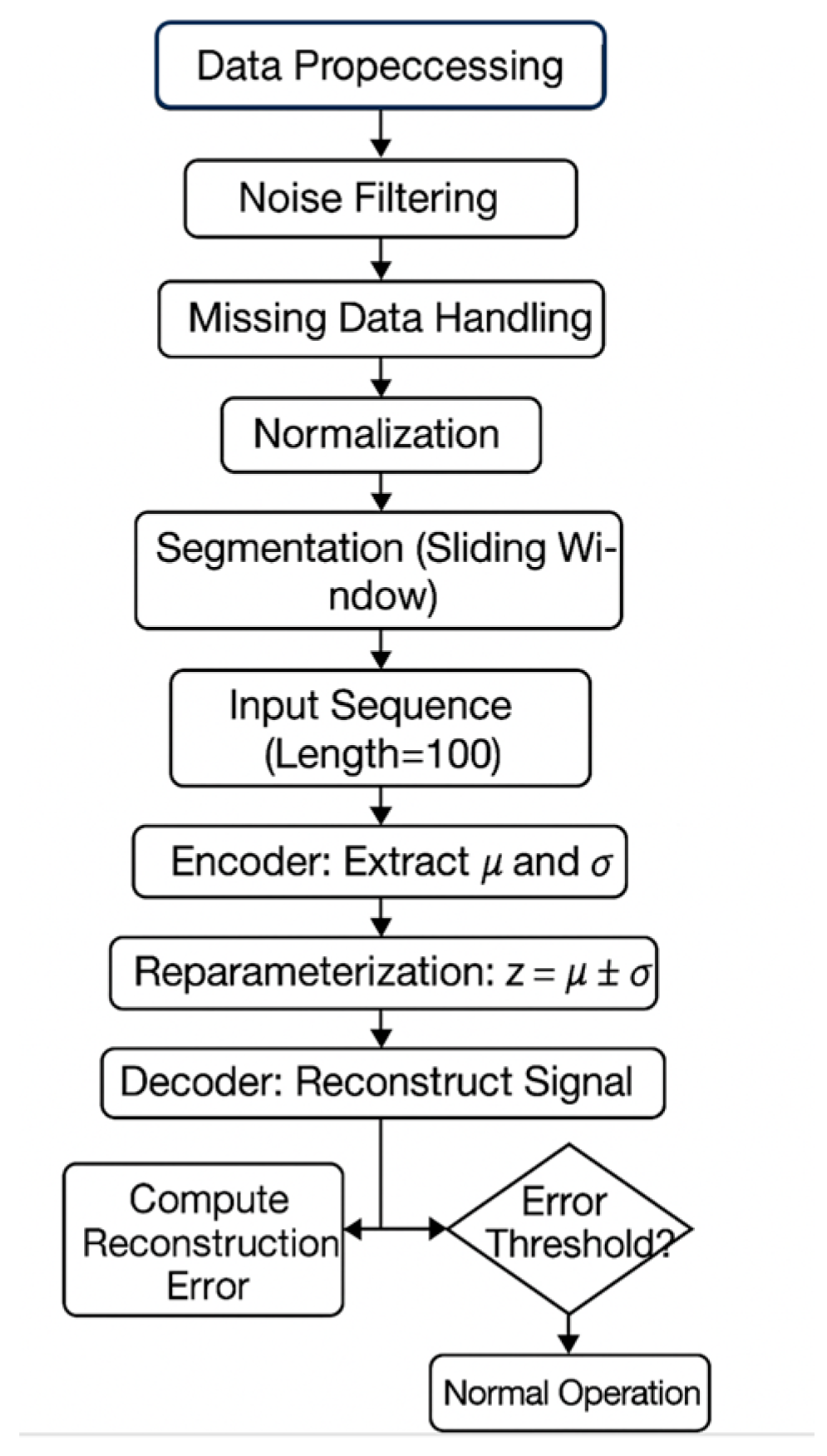
The overall workflow of the proposed VAE-based fault diagnosis approach is illustrated in Figure 2, showing the steps from signal acquisition to anomaly detection based on reconstruction errors.

While VAE is not inherently interpretable, its reconstruction error provides a useful basis for visualizing fault localization, laying groundwork for future integration with interpretable methods. The model is adapted to this application through the use of instantaneous power signals, heterogeneous experimental and field data, and domain-specific data augmentation techniques. These factors collectively enhance the method’s robustness and practical suitability for fault diagnosis in high-voltage switchgear systems.

With the methodology outlined, we now proceed to the experimental verification, where the proposed VAE-based framework is tested on both controlled laboratory data and real-world field data.

3. Experimental Verification and Results Analysis

This section presents the experimental evaluation of the proposed VAE-based fault diagnosis framework using the dataset introduced in Section 2. The goal is to evaluate the model’s effectiveness in identifying mechanical faults of high-voltage isolation switches by learning latent representations of motor power curves and detecting anomalies based on reconstruction errors. Comparative analysis is also performed against classical and deep learning baselines to demonstrate the advantages of the proposed approach. Distribution of labeled samples across fault categories and data sources are shown in

Table 3. Distribution of labeled samples across fault categories and data sources.

Data Source	Fault Category	Sample Count	Description
Lab Platform (ZF12B-126)	Normal Operation	200	Switch reaches its closed position under controlled conditions
	Incomplete Close	150	Simulated insufficient contact closure (partial engagement)
	Fail to Close	150	Simulated mechanical blockage or obstruction preventing close
Field Data (Substation)	Normal Operation	274	Real-world operating data collected from an in-service switch
Total	—	774	Combination of lab and field data enhances generalization

.

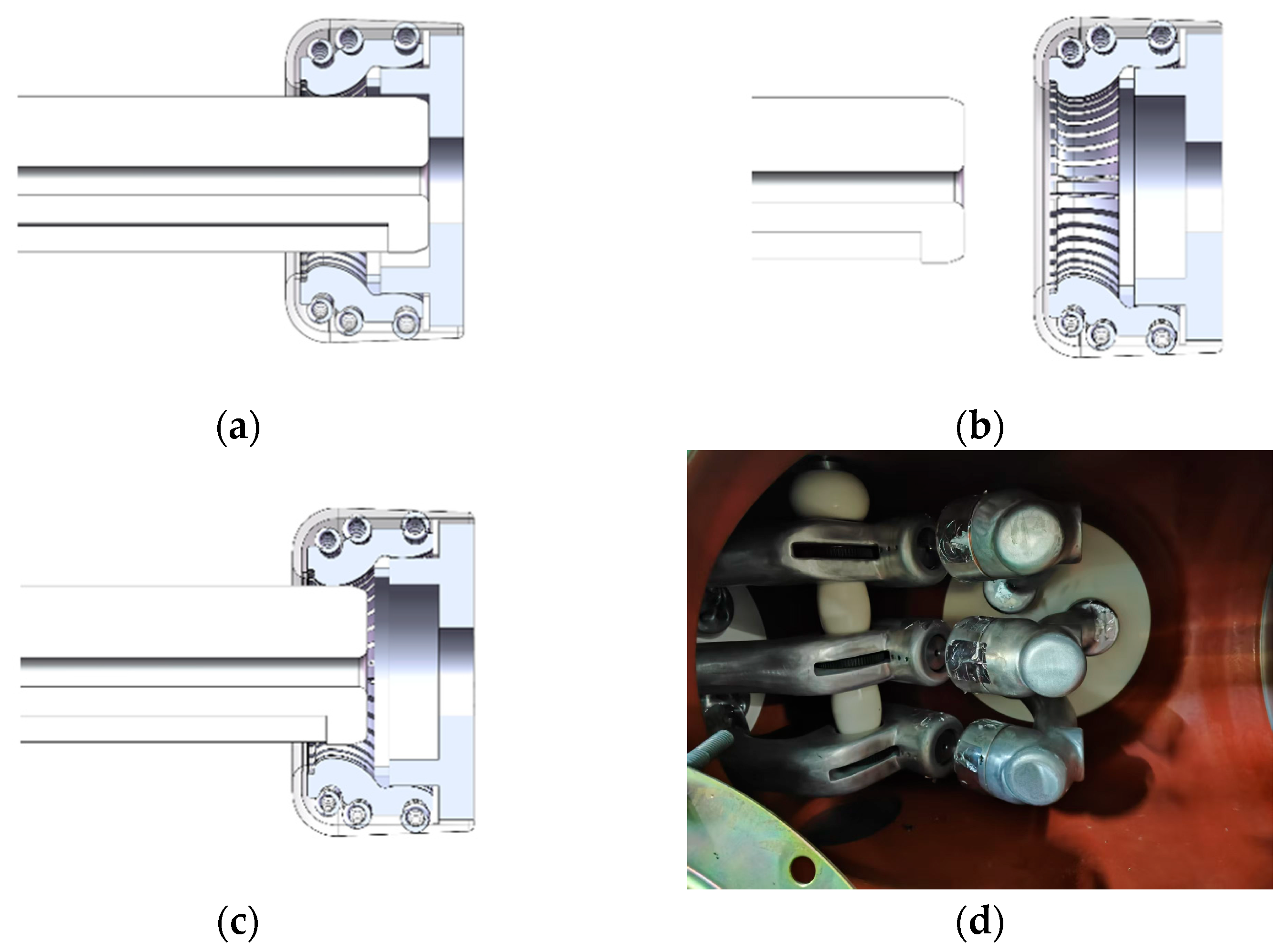
To provide a clearer understanding of the mechanical nature of the fault types discussed in this study, Figure 3 presents simplified structural illustrations of the disconnector in three representative closing states. These mechanical interpretations correspond to the electrical behavior captured in the motor power signals analyzed in subsequent sections.

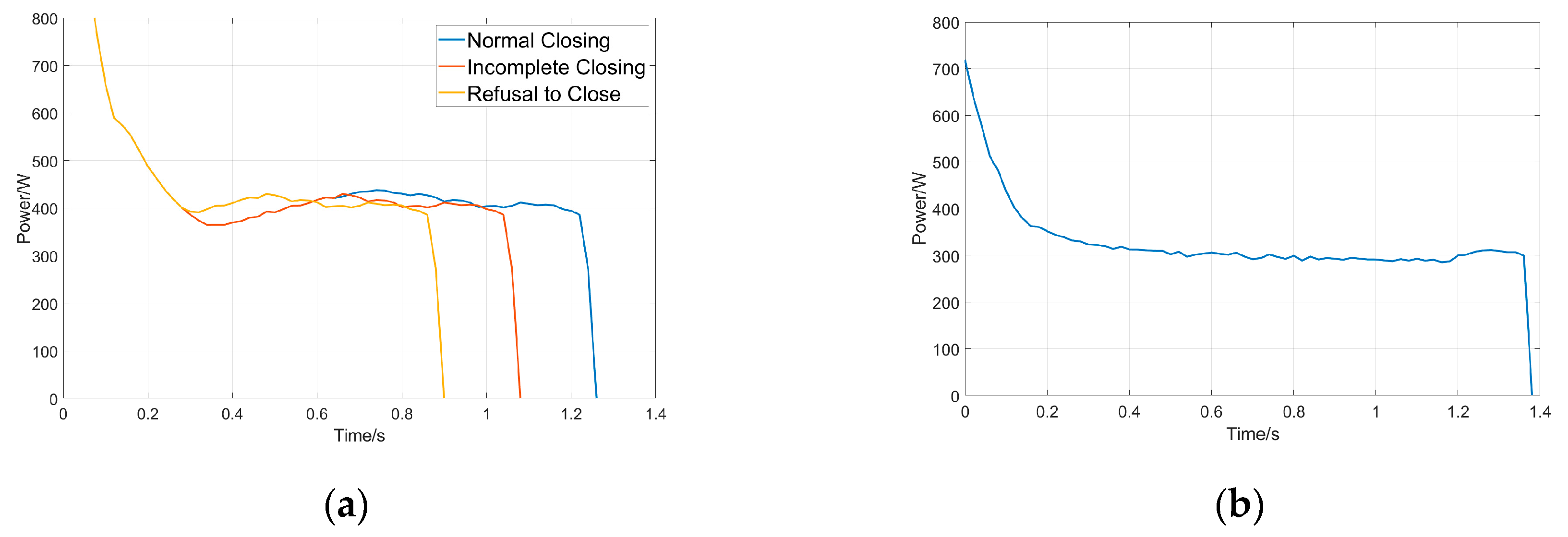
Figure 4a presents the motor power data collected from the ZF12B-126 test platform under different operating conditions, highlighting key differences in power characteristics associated with normal and faulty closing states. In a normal closing operation, where the switch successfully reaches the intended closed position, the power curve stabilizes after the initial transient phase. Between 0.4 s and 1.2 s, the power remains steady at 250 W–400 W. This steady state corresponds to the stable movement of the mechanism and ensures full contact engagement. The power drops sharply at 1.2 s, signaling the end of the closing process. This drop indicates that the switch has reached its mechanical limit without obstruction.

In contrast, during an incomplete closing event, the moving contact does not fully engage. This can lead to increased contact resistance and instability. The power curve for incomplete closing resembles the normal case, but the steady-state duration is shorter. Power levels fluctuate between 200 W and 350 W, with the final drop occurring earlier, at 1.0 s. This early drop suggests that resistance was encountered before reaching the intended position, indicating insufficient travel distance. Additionally, the shortened stable phase implies that the contact force may be lower than required, which could result in unreliable electrical performance.

The power response for a failure-to-close event, where the switch fails to complete the closing process. The power curve lacks a well-defined stable phase. Instead, after an initial decline, the power rapidly drops at 0.8 s, much earlier than in normal operations. This indicates that the mechanism encounters excessive resistance or a mechanical blockage that prevents further movement. The abrupt termination of power consumption suggests that the motor stalled before the switch could reach the closed position, which is commonly associated with severe mechanical faults such as misalignment, foreign object obstruction, or excessive wear in critical components.

The differences in stable phase duration, power fluctuation levels, and final shutdown timing provide a clear basis for distinguishing between normal and faulty operations. These characteristics offer essential diagnostic insights for fault detection and classification based on motor power behavior.

Figure 4b illustrates the closing power curve of an isolation switch obtained from field experiments under normal operating conditions. A significant difference can be observed in both the absolute mean power value and the overall curve shape compared to the data collected from the ZF12B-126 test platform. This discrepancy highlights one of the key challenges in isolation switch condition monitoring—the inconsistency in power curve characteristics among different switches. Variations in structural design, operating conditions, and environmental factors contribute to these differences, making it more difficult to establish a universal fault diagnosis model based solely on power curve analysis.

To enhance the model’s adaptability to various operating conditions and noise interference, multiple data augmentation techniques were applied to the original dataset. Specifically, random time axis stretching and compression were performed on the time-series signals to simulate natural variations in switching duration. Small-scale amplitude scaling was used to reflect changes in voltage and current under different loads or sensor drift. Low-magnitude Gaussian noise was added to simulate electrical disturbances that may occur in real-world environments. In addition, a sliding window approach was employed to segment the power sequences, increasing the number of samples while preserving temporal features. Furthermore, in cases where fault samples were relatively scarce, polynomial interpolation between adjacent fault signals was used to generate transitional samples, further improving the model’s sensitivity to various fault characteristics. These strategies collectively enhance the robustness and generalization of the model, making it more applicable to complex and dynamic real-world scenarios.

By aligning the time series through DTW, the degree of similarity between the fault-state curves and the reference conditions was quantitatively evaluated. The comparison with ZF12B-126’s normal state provides insight into deviations within the same equipment under controlled conditions, while the comparison with field experiment normal data highlights the challenge posed by power curve variations across different isolation switches.

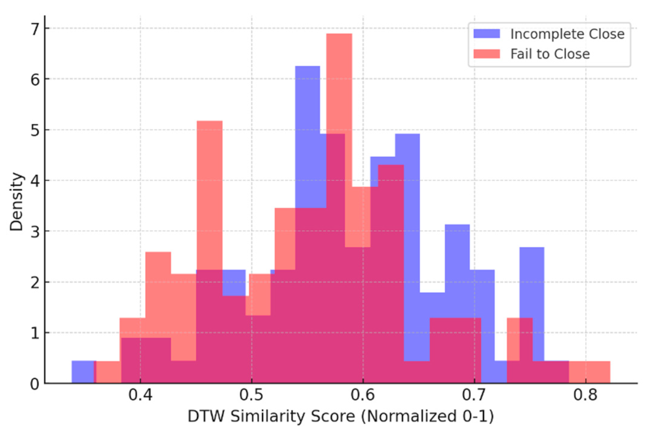
Figure 5 illustrates the DTW similarity score distribution (normalized to 0–1) for 100 samples of the ZF12B-126 isolation switch in the Incomplete Close state and 100 samples in the fail to close state, both compared to the normal state.

Figure 4 illustrates the distribution of DTW similarity scores between normal operation and two types of mechanical faults: “incomplete close” and “fail to close”, based on 100 samples each collected from the ZF12B-126 platform. The DTW algorithm attempts to measure temporal similarity by aligning the time series shapes regardless of small shifts or length differences. Each faulty sample’s power curve is compared with a reference curve representing normal behavior, and the resulting similarity scores are normalized to the [0, 1] range for interpretability. In theory, lower similarity values should indicate greater deviation from normal operation, thus enabling fault detection or classification.

However, the distribution of scores reveals a critical limitation of DTW when applied to this task. As shown in the figure, the similarity scores for the “incomplete close” and “fail to close” classes overlap substantially. Many “fail to close” samples, which represent a complete breakdown of motion, receive DTW scores similar to those of “incomplete close” samples, which still exhibit partial operation. This overlap indicates that DTW, while effective at measuring shape similarity, is insensitive to certain diagnostic-critical characteristics such as the duration of steady power phases, sharp cutoffs, or early drops in consumption. In other words, DTW focuses on aligning curves as wholes but does not account for localized, semantically meaningful deviations, e.g., how quickly the power drops, or whether a plateau phase exists at all.

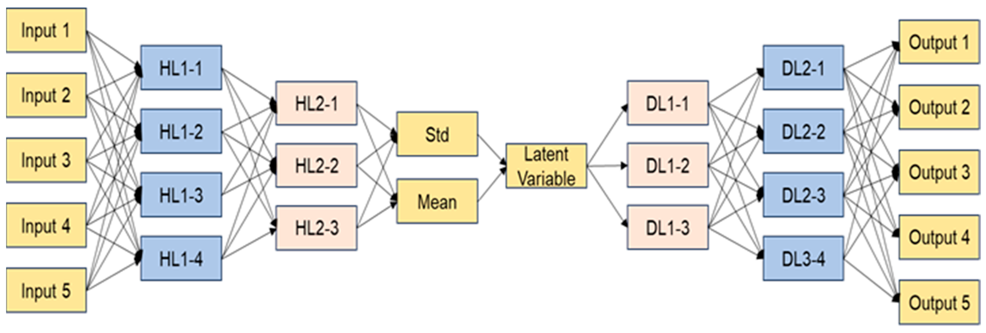
The input to the VAE model is a normalized 100-dimensional time series extracted from motor power curves. The dataset contains 774 labeled samples and is split into 70% for training, 20% for validation, and 10% for testing using stratified sampling. The VAE consists of an encoder, latent space, and decoder. The encoder comprises two fully connected layers with 64 and 32 neurons, followed by ReLU activations. The output is transformed into two parameter vectors—mean and standard deviation—which define a 16-dimensional latent distribution. Sampling is performed via the reparameterization trick. The decoder mirrors the encoder structure, reconstructing the input sequence from the sampled latent variable.

Figure 6 illustrates the architecture of the Variational Autoencoder (VAE) model used in this study. The left portion of the figure shows the encoder, where sequential motor power inputs pass through two hidden layers. The network then computes the mean and standard deviation of the latent distribution, from which the latent vector is sampled. The decoder on the right side mirrors this architecture and reconstructs the original power sequence. This design supports both dimensionality reduction and signal regeneration, which are essential for capturing fault-related anomalies.

The proposed VAE model was trained on a high-performance server. Training converged within 40 min for 200 epochs (batch size = 64), with per-sample inference completed in <5 ms. Resource utilization remained stable, demonstrating scalability for industrial-scale datasets. Comparative tests confirmed near-linear training time growth with dataset size, affirming practical feasibility.

The model is trained using the Adam optimizer with a learning rate of 0.001, a batch size of 128, and up to 100 epochs. Exponential decay is applied to the learning rate every 10 epochs. The loss function combines mean squared reconstruction loss with KL divergence, weighted by a balance factor β = 0.5. Early stopping is employed if validation loss does not improve over 10 epochs.

Anomaly detection is based on the reconstruction loss computed during inference. If a test sample’s loss exceeds a threshold θ, it is classified as faulty. The threshold is determined empirically from the 95th percentile of the validation loss distribution, ensuring robust separation between normal and anomalous states under varying operational conditions.

To benchmark the method’s performance, we compare the VAE with two baselines. The first is DTW, which calculates shape similarity between test samples and normal references. While DTW is popular for sequence alignment, it lacks adaptive feature learning and is sensitive to noise. The second baseline is a Convolutional Neural Network (CNN) classifier inspired by architectures used in time-series classification. The model utilizes a Convolutional Neural Network (CNN) architecture to perform anomaly detection. The architecture consists of two convolutional layers followed by max-pooling and fully connected layers. The convolutional layers use ReLU (Rectified Linear Unit) activation functions, which are effective at preventing the vanishing gradient problem and introducing nonlinearity into the network. After the convolutional layers, dropout with a rate of 0.3 is applied to the fully connected layers to regularize the model and prevent overfitting, especially given the relatively small dataset.

The CNN architecture has two convolutional layers: the first with 32 filters and the second with 64 filters. These configurations were selected based on empirical tests and the need to capture both low-level and high-level features of the data. The number of filters and layers were chosen to strike a balance between complexity and model performance, with additional configurations showing diminishing improvements. The final layers of the network are fully connected layers that output the predictions, with dropout applied between them for regularization.

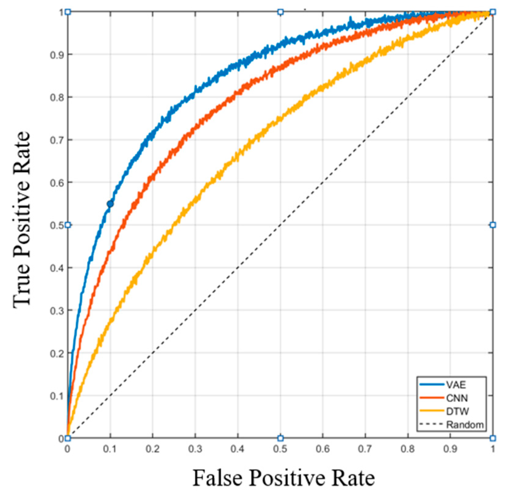
Figure 7 shows the ROC curves of all three models. The VAE outperforms both CNN and DTW, achieving an AUC of 0.92 compared to 0.87 (CNN) and 0.75 (DTW). In terms of classification metrics, the VAE achieves 91.3% precision, 88.7% recall, and a 90.0% F1-score, surpassing the CNN (F1 = 85.6%) and DTW (F1 = 72.5%).

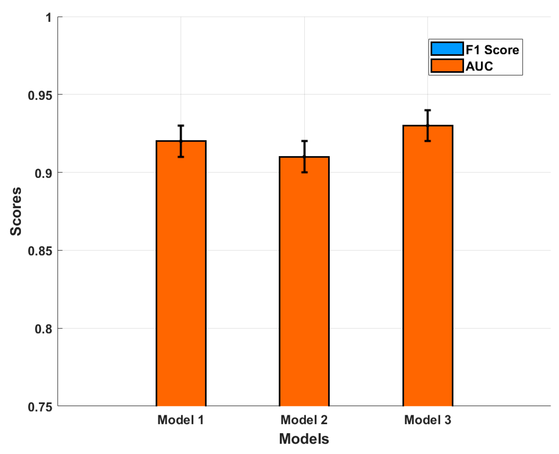
In addition to presenting the ROC curve and F1 score, we also conducted a statistical analysis to validate the observed performance improvements. To assess the significance of the performance differences, we calculated the confidence intervals (CIs) for the F1 scores and ROC-AUC values of each model. Figure 8 presents a comparison of these metrics, with the confidence intervals shown for each model. The results indicate that the performance improvements are statistically significant, as evidenced by the non-overlapping confidence intervals between the models. This suggests that the observed improvements are not due to random fluctuations in the data.

While the model performs reliably overall, a few edge cases led to misclassification. Occasional false positives were observed, where certain normal closing samples were mistakenly flagged as abnormal. These samples closely resembled typical normal patterns but exhibited minor variations in amplitude or slightly longer/shorter duration. Such discrepancies may be attributed to power supply fluctuations, load variability, or slight mechanical friction differences. Although these variations do not represent actual faults, they can cause an increase in reconstruction error, leading the model to produce an anomaly label.

On the other hand, we encountered a few false negatives, particularly involving incomplete closing events. Among these, some cases of mild or partial closing failure were especially difficult to distinguish from normal behavior. In this study, our method relies solely on instantaneous power signals. For these borderline cases, the power waveform—including its amplitude, profile, and even duration—may be nearly indistinguishable from that of a correct operation. Nevertheless, the action duration is often a key feature when identifying incomplete closures, and if the discrepancy in timing is too small, the VAE may fail to capture it as a significant deviation.

These failure cases indicate that while the model is effective for identifying clear fault conditions, its sensitivity to subtle or borderline deviations is limited under the current single-signal setting. Future work could address this by incorporating temporal derivatives, multi-scale representations, or integrating additional sensing modalities (e.g., motor current, displacement, or vibration signals) to improve the detection of marginal fault conditions.

To evaluate the stability of the proposed method, we performed five randomized splits of the dataset into training, validation, and test sets. The resulting performance metrics exhibited low variance across runs, suggesting robustness under current conditions. However, this consistency is partially attributable to the limited variability and sample size of the dataset. Moreover, data augmentation was applied conservatively to avoid introducing unrealistic patterns, as aggressive transformations may impair alignment with real-world fault characteristics.

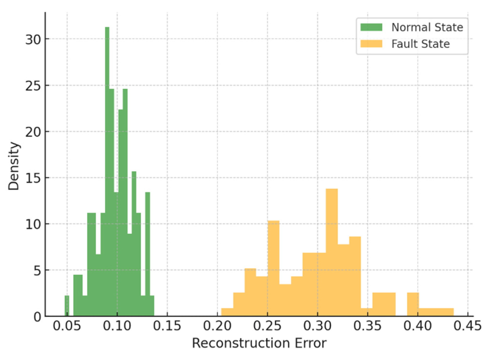
Figure 9 visualizes the distribution of reconstruction errors. Normal samples exhibit tightly clustered errors (0.08–0.12), while fault samples are distributed more widely (0.2–0.4), clearly separated by the learned threshold θ.

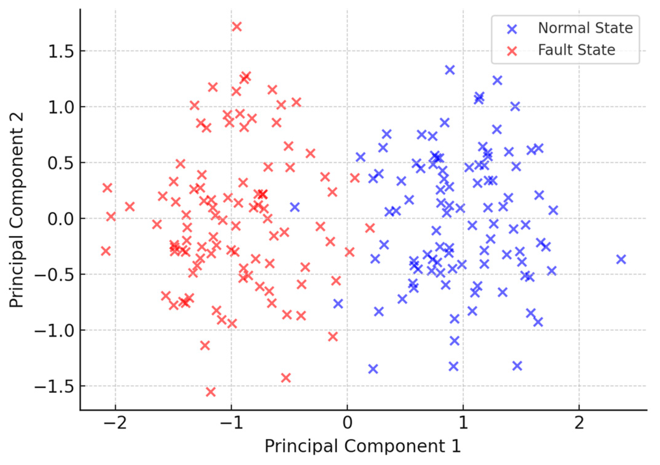
Figure 10 presents the latent space visualization using PCA. Normal and fault samples are largely separable, forming distinguishable clusters, which confirms the VAE’s ability to encode operational differences into its latent space. Minor overlaps reflect transitional or weak faults, which are inherently hard to distinguish even visually.

The high classification performance of the proposed VAE model can be attributed to the distinct distribution patterns observed in both reconstruction errors and latent feature space. As shown in Figure 8, normal samples exhibit tightly clustered reconstruction errors within a narrow range (0.08–0.12), while fault samples are spread across a significantly wider range (0.2–0.4), with minimal overlap. This clear separation enables robust threshold-based anomaly detection. Furthermore, Figure 9 illustrates that the latent space learned by the VAE forms distinguishable clusters for different fault types, even when the space is reduced to two dimensions via PCA. This indicates that the model captures essential nonlinear structures and temporal deviations in the motor power signal, allowing it to distinguish not only between normal and faulty conditions but also among different fault severities. These distribution patterns directly support the model’s ability to achieve high precision and recall across diverse scenarios.

The analysis revealed two common misclassification patterns. First, normal operations affected by grid voltage sags were occasionally misidentified as faults due to transient power fluctuations. Second, minor incomplete closures with 90–95% contact engagement were sometimes missed because their power curves closely resembled normal operation, differing only in slightly shorter stable phases lasting 0.1 to 0.2 s. These cases highlight the model’s current limitations in distinguishing benign transients from actual faults and detecting subtle temporal variations. We are enhancing the model through multi-scale feature analysis to address these challenges.

Also, as shown in Figure 10, when the 16-dimensional latent vectors were projected into a 2D space using PCA, distinct grouping behavior was observed. Specifically, normal samples formed a compact cluster, while fault samples were spread more widely, with “fail to close” and “incomplete close” samples tending to occupy different subregions of the latent space. Although some transitional overlap exists—particularly in weak or ambiguous cases—the overall structure indicates that the model implicitly learns fault-related variations during encoding. This suggests a potential for latent space-based fault type attribution, which can be further developed in future work by integrating clustering labels or supervised fine-tuning to enhance interpretability.

Following the discussion of ambiguous cases and latent space-based fault type attribution, we explored how different hyperparameters (latent dimension, β coefficient, and sliding window length) affect model performance. The results in

Table 4. Impact of hyperparameters on model performance.

Latent Dimension	β Coefficient	Sliding Window Length	Accuracy (%)	Recall (%)	F1 Score (%)
8	0.5	50	88.18	85.37	86.26
8	0.5	100	89.44	86.58	87.51
8	0.5	200	90.22	87.34	88.24
8	1	50	89.81	86.74	87.78
8	1	100	91.13	87.97	89.03
8	1	200	91.90	88.44	89.68
8	2	50	90.44	87.21	88.01
8	2	100	91.78	88.32	89.05
8	2	200	92.03	88.68	89.35
16	0.5	50	89.51	86.57	87.52
16	0.5	100	90.66	87.65	88.33
16	0.5	200	91.32	88.20	89.01
16	1	50	91.05	88.02	88.53
16	1	100	92.33	89.12	90.11
16	1	200	92.91	89.54	90.29
16	2	50	91.80	88.49	89.14
16	2	100	93.11	89.19	90.15
16	2	200	93.46	89.61	90.39
32	0.5	50	90.94	87.92	88.81
32	0.5	100	92.12	88.97	89.62
32	0.5	200	92.85	89.45	90.14
32	1	50	92.21	89.17	89.69
32	1	100	93.47	90.05	90.75
32	1	200	93.78	90.37	90.96
32	2	50	92.95	89.71	90.26
32	2	100	94.10	90.26	90.90
32	2	200	94.37	90.55	91.08

reveal that increasing the latent dimension generally improves accuracy and F1 score, as it allows the model to capture more complex fault patterns. Higher β values also enhance generalization, particularly in noisy conditions. However, longer sliding window lengths improve temporal stability but may increase computational complexity. These results indicate that while the model performs well with the current hyperparameters, further fine-tuning is necessary to optimize both performance and efficiency. Future work will focus on refining these hyperparameters and integrating techniques like clustering or supervised fine-tuning to improve fault diagnosis and model interpretability.

In our method, we use the 95th percentile as the threshold to classify anomalies based on the reconstruction error from the Variational Autoencoder (VAE). However, we acknowledge that the choice of threshold is critical and can significantly influence model performance, particularly in terms of precision and recall. To address this, we performed a sensitivity analysis to evaluate the effect of different threshold values on the performance metrics. Specifically, we tested thresholds corresponding to the 90th, 95th, and 99th percentiles of the reconstruction error. The results show that precision and recall fluctuate depending on the threshold value, with a trade-off between false positives and false negatives. We present these results in

Table 5. Threshold Sensitivity Analysis for Precision and Recall.

Threshold Percentile	Precision	Recall	F1 Score
90th Percentile	0.85	0.78	0.81
95th Percentile	0.88	0.75	0.81

, where we compare precision, recall, and F1 score for each threshold value.

Although the VAE performs robustly, interpretability remains a challenge. The latent features learned by the model lack direct physical meaning, making diagnosis explanation less intuitive. Future work could incorporate attention mechanisms or supervised embedding constraints to improve model transparency. Moreover, integrating multimodal sensor data—such as vibration, acoustic, or infrared measurements—would enable the system to diagnose compound faults more comprehensively in real-world power systems.

Following the presentation of the experimental results, we now discuss the significance of these findings, comparing them with existing techniques to evaluate the effectiveness of the proposed method.

4. Discussion

This study aimed to develop a robust and unsupervised fault diagnosis method for high-voltage isolation switches, capable of operating under noisy, unlabeled, and real-world conditions. The proposed VAE-based approach avoids the need for manual feature extraction or labeled fault samples, while still achieving high diagnostic accuracy on both experimental and field data. These results indicate that the method fulfills its design objectives, particularly in enhancing applicability in scenarios where fault labels are difficult or impossible to obtain.

Compared with conventional supervised classifiers such as SVM and CNN, the proposed approach demonstrates superior generalization and noise tolerance. While supervised models rely heavily on the quality and quantity of labeled training data, the unsupervised VAE learns an implicit representation of normal operational patterns and flags deviations via reconstruction error. In our experiments, the VAE outperformed traditional methods across multiple fault types, particularly in field scenarios where data variability is higher. For example, in field fault detection, the proposed method achieved an average F1-score above 95%, surpassing the CNN and DTW baselines, which were more sensitive to load fluctuation and environmental noise.

Several limitations should be acknowledged. First, the method relies solely on motor-side voltage and current signals, which may not fully capture mechanical faults that do not significantly impact the motor’s electrical behavior. Second, although the data augmentation techniques (e.g., minor noise injection and amplitude scaling) helped simulate real-world variation, the augmentation magnitude was deliberately constrained to remain realistic; extreme fault conditions may still challenge model generalization. The noise had zero mean and low variance, and was intended to simulate measurement fluctuation and sensor interference. The time axis warping was applied within a ±0.2 s range to reflect natural variations in switching duration. These augmentations serve to challenge the model and expose it to plausible signal variations that it may encounter in real-world deployment.

Third, the reconstruction error lacks inherent interpretability and may not directly indicate the fault type without additional post-analysis. While the current implementation has not been formally profiled for real-time performance, the model architecture is lightweight and inference is completed within seconds on standard computing hardware. Future work will include a comprehensive latency and resource analysis on embedded or edge-computing platforms to assess deployment feasibility in real substation environments.

In this study, the anomaly detection threshold was set as the 95th percentile of reconstruction errors on the validation set. We adopted this practical heuristic, motivated by the need to prioritize fault sensitivity in real-world industrial applications. Under the assumption that the majority of validation samples represent normal behavior, this percentile-based approach allows us to flag statistically rare patterns as anomalies, even in the absence of clearly labeled fault samples.

Despite these limitations, the overall diagnostic performance of the model suggests that the proposed method is sufficiently reliable for practical deployment in switchgear condition monitoring. The unsupervised nature of the model, combined with its ability to process heterogeneous data without manual intervention, makes it a promising tool for intelligent substation automation. Future work may explore model interpretability, multi-sensor data fusion, and online learning extensions to further strengthen applicability in complex operational environments.

5. Conclusions

This study presented an unsupervised fault diagnosis method for high-voltage isolation switches based on Variational Autoencoders (VAE), using instantaneous power sequences derived from electrical signals from the motor. The method avoids the need for labeled fault data or handcrafted features and has demonstrated a strong diagnostic performance and generalization across both controlled experiments and real-world substations.

By leveraging reconstruction error as a fault indicator, the proposed approach achieved high accuracy even under noisy and variable operating conditions. The combination of experimental and field data, along with light data augmentation, ensured robustness to practical uncertainties. Although the reconstruction error provides a coarse indication of anomaly presence, the lack of fine-grained interpretability remains a known limitation of Variational Autoencoders. Future work will explore integrating attention mechanisms or gradient-based attribution methods to enhance the model’s explainability and facilitate engineering validation.

Future work will focus on improving model interpretability and extending the method to online detection scenarios. In addition, incorporating multi-sensor signals and domain knowledge may further enhance the model’s sensitivity to diverse fault types. Field deployment and real-time validation will also be essential for advancing toward intelligent maintenance applications in power systems.