Predictive Framework for Membrane Fouling in Full-Scale Membrane Bioreactors (MBRs): Integrating AI-Driven Feature Engineering and Explainable AI (XAI)

Abstract

Membrane fouling remains a major challenge in full-scale membrane bioreactor (MBR) systems, reducing operational efficiency and increasing maintenance needs. This study introduces a predictive and analytic framework for membrane fouling by integrating artificial intelligence (AI)-driven feature engineering and explainable AI (XAI) using real-world data from an MBR treating food processing wastewater. The framework refines the target parameter to specific flux (flux/transmembrane pressure (TMP)), incorporates chemical oxygen demand (COD) removal efficiency to reflect biological performance, and applies a moving average function to capture temporal fouling dynamics. Among tested models, CatBoost achieved the highest predictive accuracy (R² = 0.8374), outperforming traditional statistical and other machine learning models. XAI analysis identified the food-to-microorganism (F/M) ratio and mixed liquor suspended solids (MLSSs) as the most influential variables affecting fouling. This robust and interpretable approach enables proactive fouling prediction and supports informed decision making in practical MBR operations, even with limited data. The methodology establishes a foundation for future integration with real-time monitoring and adaptive control, contributing to more sustainable and efficient membrane-based wastewater treatment operations. However, this study is based on data from a single full-scale MBR treating food processing wastewater and lacks severe fouling or cleaning events, so further validation with diverse datasets is needed to confirm broader applicability.

1. Introduction

Membrane bioreactor (MBR) technology has emerged as a crucial innovation in the wastewater treatment industry, offering significant advantages over conventional activated sludge processes. MBRs combine biological treatment with membrane filtration, resulting in high-quality effluent suitable for various reuse applications [1,2]. The process is characterized by its compact footprint, reduced sludge production, and superior removal of contaminants, including micropollutants and pathogens [3]. These benefits have led to the widespread adoption of MBRs in both municipal and industrial wastewater treatment facilities worldwide. However, MBR technology faces a persistent challenge: membrane fouling [4,5]. Fouling results from the accumulation of particles, colloids, and dissolved substances on or within the membrane, causing decreased permeability, increased energy consumption, and more frequent cleaning or replacement. It is influenced by factors such as influent wastewater characteristics, operational conditions, and biomass properties [6,7,8], ultimately impacting operational efficiency and significantly increasing maintenance costs. As the industry evolves, innovative solutions and predictive tools are needed to address fouling and optimize MBR performance for long-term sustainability.

The prediction of membrane fouling in MBR processes has become increasingly crucial for optimizing operational efficiency and reducing maintenance costs. Accurate fouling prediction allows operators to implement proactive measures, such as adjusting operational parameters or scheduling cleaning interventions, to mitigate the negative impacts of fouling on system performance [9,10,11,12,13,14]. Effective treatment of diverse wastewaters requires optimizing process design and operational conditions to minimize membrane fouling. Given its flux-driven nature, operating at excessively high flux may reduce cleaning frequency temporarily but accelerate fouling, raising long-term costs and risks [9]. Accurate fouling prediction enables the selection of operating conditions that balance productivity, effluent quality, cleaning needs, and overall cost. This highlights the role of predictive tools in achieving sustainable and economical MBR operation. Traditional approaches to fouling prediction have relied on empirical models and laboratory-scale experiments, which often fail to capture the complex dynamics of full-scale MBR systems. In recent years, researchers have explored various advanced techniques to enhance fouling prediction accuracy [10,11]. Mechanistic models based on principles of fluid dynamics, mass transfer, and biofilm formation have been developed to simulate the intricate interactions between biomass, suspended solids, and membrane surfaces, providing insights into fouling mechanisms [12]. Statistical and data-driven approaches, including time-series analysis and multivariate techniques, have also been used to identify correlations and detect trends in membrane performance [13,14]. Additionally, researchers have investigated the use of online monitoring tools and sensors to provide real-time data on key fouling indicators, such as transmembrane pressure (TMP) and permeate flux [15,16]. While these methods have shown promise in specific applications, they often face limitations when applied to the diverse and dynamic conditions encountered in full-scale MBR operations. The complexity of the fouling process, influenced by numerous interrelated factors, poses a significant challenge to developing universally applicable prediction models. Moreover, the time-dependent nature of fouling and the potential for sudden changes in influent characteristics or operational conditions further complicate prediction [17,18]. As a result, there is a growing recognition of the need for more sophisticated and adaptable approaches to membrane fouling prediction in MBR systems.

Artificial intelligence (AI) has emerged as a powerful tool for predicting membrane fouling in MBR systems, offering several advantages over traditional methods [19,20,21,22,23,24]. AI-based approaches, particularly machine learning algorithms, can effectively handle complex non-linear relationships between multiple variables and capture hidden patterns in large datasets [25,26,27,28]. These techniques have demonstrated superior predictive performance compared to conventional statistical models, especially when dealing with the dynamic and multifaceted nature of MBR fouling. However, most previous applications have been validated primarily under controlled laboratory or pilot-scale conditions, with limited demonstration in the noisy and dynamic environments of full-scale MBRs. Various AI algorithms have been applied to MBR fouling prediction, including artificial neural networks (ANNs), support vector machines (SVMs), random forests, and, more recently, deep learning models [19,20,21,22,23,24]. These models typically utilize a range of input parameters to predict fouling indicators, such as TMP or permeate flux. Common input variables include operational parameters (e.g., aeration rate, flux, MLSS concentration), influent characteristics (e.g., chemical oxygen demand (COD), nutrients, temperature), and membrane properties. Some studies have also incorporated advanced feature engineering techniques to enhance model performance, such as principal component analysis (PCA) for dimensionality reduction or wavelet transforms for time-series analysis [25,26]. The selection of appropriate input parameters and target variables is crucial for developing accurate and robust AI models. Researchers have explored various combinations of parameters, with some focusing on easily measurable online data, while others incorporate more comprehensive sets of physicochemical and biological indicators [27,28].

Despite the promising results achieved by AI-based fouling prediction models, several limitations and challenges persist, particularly regarding their robustness and generalizability when transitioning from controlled experimental settings to real-world full-scale MBR operations. One significant drawback is the “black box” nature of many AI algorithms, particularly deep learning models, which can make it difficult for operators to understand and trust the predictions [29,30,31]. This lack of interpretability can hinder the adoption of AI models in practical MBR operations, where operators need to make informed decisions based on model outputs. Another challenge lies in the quality and representativeness of the data used to train AI models. Many studies rely on data collected from well-controlled laboratory experiments or pilot-scale systems, which, unlike real-world full-scale MBR operations, often lack the noise, missing values, and operational variability encountered in practice. As a result, AI models developed under such conditions may not perform reliably when applied to real-world data, highlighting the need for approaches validated in actual operational environments. The issue of data scaling and normalization is also critical, as different input parameters often have vastly different ranges and units, potentially leading to biased or inaccurate predictions if not properly addressed. This is especially true considering the significant variability in the characteristics of wastewater treatment plant data [32,33]. Membrane fouling exhibits a time-dependent nature not only in MBR processes, but also in most membrane processes [34,35,36]. To capture the time-dependent nature of fouling, AI models must use feature engineering that accounts for both current and historical operational data. Most existing methods overlook the cumulative effects of past conditions, underscoring the need for advanced techniques that incorporate temporal dependencies and long-term trends in MBR performance. Another consideration is the choice of target parameter for fouling prediction. To date, the most commonly used representative target parameters (i.e., outputs) for predicting membrane fouling based on AI are TMP and flux [37,38,39,40]. In the case of TMP, when the operation mode of the MBR process is constant flux mode, it increases as membrane fouling progresses; conversely, in the case of flux, when the operation mode is constant pressure mode, it decreases as membrane fouling progresses [41,42,43]. In most cases, MBR processes are operated in constant flux mode [44,45]. However, due to inflow variability and changing environmental conditions, both flux and TMP often fluctuate even under constant flux operation. Therefore, it is important to select target parameters that reflect these simultaneous variations. Further research should focus on identifying such parameters to provide more accurate and practical insights into membrane fouling and to improve prediction performance. Continued efforts to enhance model interpretability, data quality, and feature engineering are essential for advancing AI-based fouling prediction and its practical application in MBR operations.

The primary objective of this study is to develop a predictive framework for membrane fouling in full-scale MBRs by integrating AI-driven feature engineering and explainable AI (XAI). To achieve this, the research focuses on innovative modeling strategies that enhance both prediction accuracy and practical applicability under real-world operating conditions. This study prioritizes parameters measurable in resource-constrained field environments, avoiding reliance on idealized or synthetic data. The proposed AI-driven feature engineering techniques (e.g., moving averages) explicitly address challenges like sensor noise and infrequent sampling, ensuring relevance to real-world MBR operations. This approach is distinguished by several innovative elements. First, diverse feature engineering techniques are employed to extract meaningful information from raw data, effectively capturing the complex relationships between operational parameters and fouling behavior. Additionally, specific flux (flux/TMP), which is physically equivalent to membrane permeability, is introduced as the target parameter. This dynamic indicator comprehensively reflects membrane performance by simultaneously accounting for variations in both flux and transmembrane pressure. Furthermore, COD removal efficiency is incorporated as an input parameter, reflecting the biological performance of the MBR system and its potential impact on fouling. To account for the time-dependent effects of biological reactions on membrane fouling, a moving average concept is implemented in the selection of input–output data pairs. Moreover, explainable AI models are utilized to enhance operator decision support, thereby improving the interpretability and trustworthiness of fouling predictions. The applicability of the model is demonstrated using over six months of real-world data collected from an operational MBR process, rather than a designed MBR process for this study. This ensures the model’s relevance to the actual data conditions and the non-ideal circumstances present in the field. While physics-based models provide a fundamental understanding of fouling mechanisms and traditional sensing tools offer real-time monitoring, the proposed AI framework complements these approaches by translating complex operational data into actionable insights for proactive control. By integrating with existing sensor networks, the framework can enhance decision making without replacing established physical models, thereby creating a more robust MBR management system. For example, the AI model can receive real-time sensor data (e.g., TMP, DO) and dynamically adjust input parameters for physics-based simulations, enabling adaptive and responsive fouling prediction. By combining AI predictions with traditional fouling indicators, a hybrid alarm or decision support system can be established, leveraging the strengths of both data-driven and mechanistic approaches. Overall, this research makes a significant contribution to the field by presenting a robust and interpretable predictive framework for membrane fouling in full-scale MBRs, integrating AI-driven feature engineering and explainable AI. This approach lays the foundation for more effective membrane fouling management and supports sustainable improvements in MBR operations.

2. Materials and Methods

2.1. MBR Process (Data Collection)

A schematic diagram illustrating the full-scale food processing wastewater treatment process located in Beijing is presented in Figure 1. The treatment train comprises a settling tank, grate tank, equalization tank, two sequential micro-aerobic reactors, a membrane bioreactor (MBR) system, and an effluent tank. Figure 1 also delineates—in red text—the specific parameters and locations at which operational and water quality data were collected. These parameters represent the measurement points utilized for the development of the AI-driven fouling analytic and predictive framework in this study. In this study, the primary focus is placed on the membrane bioreactor (MBR) system, and the AI-driven fouling analytic and predictive framework was developed exclusively using data directly associated with the MBR process. Therefore, detailed descriptions of other unit processes depicted in Figure 1, apart from the MBR system, are not provided. It is noteworthy that all data were compiled from routine field operations under real-world conditions, rather than from laboratory or specially designed experimental scenarios. This approach ensures the practical relevance and applicability of the data for predictive modeling in full-scale MBR systems. The MBR system has a daily treatment capacity of 150 m³/d, which meets the processing requirements of the food processing plant. The main components of the MBR system include the membrane module, influent and effluent systems, aeration system, and recirculation system. Polyethylene-embedded hollow fiber membranes with a pore size smaller than 0.4 μm are used in the MBR module. These membranes have an inner and outer diameter of 0.41 mm and 0.65 mm, respectively, with an elongation rate (i.e., the maximum strain the hollow fiber membrane can withstand before failure) of less than 17%. The filtrable surface area of a single membrane group is 200.7 m², with a total of 9 membrane groups in operation. The average influent flow rate to the MBR system is 114 m³/d, with a hydraulic retention time (HRT) of approximately 0.75 days. The dissolved oxygen (DO) concentration is 5.43 mg/L, and the mixed liquor suspended solids (MLSSs) concentration ranges from 5000 to 9000 mg/L. During the monitoring period, no intentional sludge wasting was performed, and the system operated with a stable MLSS concentration. As a result, solid retention time (SRT) was not explicitly controlled or recorded. Intermittent filtration of the effluent is performed by pumps, with a pumping cycle of 10 min on and 5 min off. Membrane cleaning cycle is scheduled when the TMP increases by more than 30% from its baseline value, or when it exceeds 60 kPa, in line with most common submerged MBR operational practice [4,5]. However, no chemical cleaning events, such as chemical-enhanced backwash (CEB) or cleaning in place (CIP), occurred during the 194-day monitoring period because TMP did not exceed the established cleaning thresholds. Thus, the predictive modeling framework does not include data related to chemical cleaning events as input variables.

Samples obtained from the mixed liquor of the MBR reactor were filtered through a 0.45 μm mixed cellulose filter (Advantec, Tokyo, Japan) for COD analysis. The COD was measured according to the guidelines outlined in the Standard Methods for the Examination of Water and Wastewater [46] published by the American Public Health Association (APHA). The concentrations of the COD before and after treatment were measured using a COD meter (DR1010, HACH, Loveland, CO, USA). pH and temperature (Temp.) were quantitatively analyzed using a portable multifunctional electrode (Multi 3630, Munich, Germany) equipped with a meter-matching network. Dissolved oxygen (DO) concentrations were measured using a portable multimeter (PHB-4, Zsynet, Shanghai, China). The MLSS concentration was determined using the gravimetric method. The TMP and flow rate were monitored and recorded daily using pressure gauges and flow meters connected to the operational MBR system. The sludge volume (SV30), sludge volume index (SVI), food-to-microorganism ratio (F/M), and flux were analyzed according to standard methods.

All measurements were collected on a daily basis over a period of 194 days, ensuring a comprehensive dataset for model development. Parameters such as F/M, SV30, SVI, MLSSs, and COD were measured once per day and recorded as daily data points, while variables monitored continuously by online sensors—including DO, pH, temperature, TMP, and flowrate—were processed as daily average values to ensure consistency and comparability across the dataset. Data collection was conducted under actual field conditions typical of real-world MBR operations, where manual sampling and sensor limitations constrained the availability of high-frequency data. Accordingly, variables such as F/M, SV30, SVI, MLSSs, and COD were sampled once daily, and continuously monitored parameters were averaged to daily values to ensure data completeness and comparability. While this approach may obscure short-term fluctuations relevant to fouling dynamics, a moving average transformation (see Section 2.3.2) was applied to key features to better capture temporal dependencies and mitigate the loss of meaningful trends associated with short-term variability. These limitations, along with their implications, are discussed earlier in this section (see also Section 2.1). If high-frequency data become available in future work, visualizing intra-day trends could further enhance the analysis and interpretation of fouling behavior. The target parameters were either TMP or specific flux (Spec. Flux). Spec. Flux (=flux/TMP) is used as a target variable because it directly represents membrane permeability, a key indicator of fouling severity. In actual MBR operations, even under constant flux mode, both flux and TMP are subject to variation due to operational and environmental fluctuations [37,38]. Thus, Spec. Flux captures these simultaneous changes more effectively than either parameter alone, making it a more practical and robust indicator for predictive modeling. As fouling progresses, TMP increases for a given flux, resulting in a decrease in Spec. Flux. This inverse relationship is well established in membrane science [38,39,40]. To systematically compare model performance, four different cases were defined based on the inclusion of COD removal efficiency (COD RM) as an additional feature and the choice of the target parameters (

Table 1. Cases for model comparison based on MBR process data and target parameters.

Cases	Factors	Target
Case I	F/M, SV30, SVI, MLSSs, DO, pH, Temp.	TMP
Case II	F/M, SV30, SVI, MLSSs, DO, pH, Temp., COD RM	TMP
Case III	F/M, SV30, SVI, MLSSs, DO, pH, Temp.	Spec. Flux
Case IV	F/M, SV30, SVI, MLSSs, DO, pH, Temp., COD RM	Spec. Flux

).

2.2. Exploratory Data Analysis (EDA)

Exploratory Data Analysis (EDA) was conducted to examine the distribution, relationships, and underlying patterns in the dataset. The analysis included descriptive statistics, visualization techniques, correlation analysis, and normality tests to assess the characteristics of the features and target parameters before model development.

2.2.1. Operational Feature Statistics

Descriptive statistical measures, including mean, median, standard deviation (std), minimum, and maximum values, were calculated for all features and target variables. This analysis provided an overview of the central tendency and variability of the data, ensuring that potential anomalies or outliers could be identified.

2.2.2. Pair Plot

To investigate the pairwise relationships between features and target parameters, a pair plot was generated. This visualization provides insights into potential linear or non-linear correlations, clustering patterns, and outliers, facilitating a deeper understanding of the dataset before model development. Pair plots were constructed using the Seaborn library (0.13.2) in Python (3.13.1), incorporating regression lines to observe possible linear trends and confidence intervals to assess variability.

2.2.3. Scatter Plot

Individual scatter plots were used to explore the relationship between specific input features and target parameters (TMP and Spec. Flux). These plots helped in detecting possible linear or non-linear trends, as well as outliers that might influence model performance.

2.2.4. Pearson Correlation

The Pearson correlation coefficient (r) was computed to quantify the linear relationship between each feature and the target parameters. A correlation matrix was constructed to visualize the strength and direction of the associations. The analysis helped in feature selection by identifying highly correlated variables that could impact model performance.

2.2.5. Normality Check

To assess the normality of the dataset, the Shapiro–Wilk test was conducted for all features and target variables. The test evaluates whether a given dataset follows a normal distribution, with the null hypothesis (H₀) assuming normality and the alternative hypothesis (H₁) suggesting deviation from normality. The Shapiro–Wilk test examines statistic ranges from 0 to 1, with values approaching 1 indicating a closer resemblance to a normal distribution. A p-value threshold of 0.05 was used to assess statistical significance. If the p-value exceeded 0.05, the null hypothesis was not rejected, confirming that the data followed a normal distribution.

2.3. Preprocessing and Feature Engineering

To enhance data consistency and improve model performance under non-ideal field conditions, robust scaling and moving average transformations were applied. Robust scaling and moving averages were applied to simulate realistic field conditions, where data quality is often compromised. These methods ensure model resilience to outliers and temporal gaps, critical for industrial deployment. The following subsections detail these techniques.

2.3.1. Robust Scaling

Robust scaling was applied to normalize the dataset while reducing the influence of extreme values. Unlike standard normalization methods, which are sensitive to outliers, robust scaling centers the data around the median and scales it using the interquartile range (IQR, Q3–Q1). This method ensures that the distribution of variables with different scales remains comparable.

The transformation was performed using the following Equation (1).

$$x_{robust scaled}={\displaystyle \frac{x-Median}{Q3-Q1}}$$

(1)

2.3.2. Moving Average

In MBR processes, the removal of contaminants requires a specific processing time, leading to a time delay between influent and effluent characteristics. It should be noted that the time delay concept applied in this study is a data-driven feature engineering method designed to optimize input–output data pairing for model training, rather than a direct representation of HRT or physical process lag. This approach enables the identification of the most effective temporal alignment for fouling prediction under the given operational and data conditions. To incorporate this time-dependent behavior, a moving average transformation was applied to all features, improving the model’s ability to capture long-term trends while minimizing the effect of short-term fluctuations.

Additionally, the moving average reduces the influence of extreme values, making it particularly effective for datasets with high noise levels. The transformed value was computed as follows (Equation (2)).

$${MA}_t={\displaystyle \frac{x_{n-t+1}+x_{n-t+2}+\cdots +x_n}{t}}={\displaystyle \frac{1}{t}}{\sum }_{n-t+1}^n{x}_i$$

(2)

2.4. Models

To develop predictive models for membrane fouling, both statistical regression models and machine learning models were employed. The statistical models aimed to capture linear relationships between input features and target parameters, while machine learning models leveraged non-linear patterns to enhance predictive accuracy.

2.4.1. Statistical Models

• Linear Regression

Linear regression is a fundamental statistical approach used to model the relationship between a dependent variable Y and multiple independent variables Xi. The model is represented as follows (Equation (3)):

$$Y={\beta }_0+{\beta }_1{X}_1+{\beta }_2{X}_2+\cdots +{\beta }_p{X}_p+ϵ$$

(3)

where β₀ is the intercept, β₁ to β_p are the regression coefficients, and ϵ represents the error term. This model assumes a linear relationship between predictors and the target parameters.

2.

Lasso Regression

Least Absolute Shrinkage and Selection Operator (Lasso) regression introduces an L1 regularization term to the linear regression model, effectively performing feature selection by penalizing the absolute magnitude of regression coefficients. The objective function is defined as follows (Equation (4)):

$${\mathrm{m}\mathrm{i}\mathrm{n}}_{\beta }{\sum }_{i=1}^n{(y_i-{\beta }_0-{\sum }_{j=1}^p{\beta }_j{\beta x}_{ij})}^2+\lambda {\sum }_{j=1}^p\left|{\beta }_j\right|$$

(4)

where λ is the hyperparameter controlling the strength of regularization. Lasso regression helps mitigate overfitting by shrinking some coefficients to zero, thereby selecting only the most relevant features.

3.

Ridge Regression

Ridge regression extends linear regression by incorporating an L2 regularization term, which penalizes large regression coefficients and reduces model variance. The objective function is given by (Equation (5)).

$${\mathrm{m}\mathrm{i}\mathrm{n}}_{\beta }{\sum }_{i=1}^n{(y_i-{\beta }_0-{\sum }_{j=1}^p{\beta }_j{\beta x}_{ij})}^2+\lambda {\sum }_{j=1}^p{\beta }_j^2$$

(5)

Ridge regression is particularly useful in addressing multicollinearity issues, ensuring model stability and improved generalization.

4.

Elastic Net Regression

Elastic net regression combines L1 (Lasso) and L2 (Ridge) regularization techniques, leveraging the advantages of both. The objective function is formulated as follows (Equation (6)):

$${\mathrm{m}\mathrm{i}\mathrm{n}}_{\beta }{\sum }_{i=1}^n{(y_i-{\beta }_0-{\sum }_{j=1}^p{\beta }_j{\beta x}_{ij})}^2+\lambda (\alpha {\sum }_{j=1}^p\left|{\beta }_j\right|+{\displaystyle \frac{1-\alpha }{2}}{\sum }_{j=1}^p{\beta }_j^2)$$

(6)

where α controls the balance between L1 and L2 penalties and λ determines the overall regularization strength. This model is particularly effective when dealing with high-dimensional datasets with correlated features.

2.4.2. Machine Learning Models

The machine learning (ML) model employed in this study follows a systematic multi-stage workflow designed to ensure both predictive accuracy and interpretability. The key procedural steps are outlined as follows:

• Input: Preprocessed features, including variables such as the F/M ratio, MLSSs, and moving averages of operational parameters, are fed into the algorithm.
• Training: The algorithm iteratively builds decision trees, optimizing for minimal prediction error while penalizing overfitting.
• Output: Predictions of specific flux (flux/TMP) are generated, directly quantifying fouling severity.
• Interpretation: Shapley Additive Explanation (SHAP) values quantify the contribution of each input variable to predictions, enabling operators to identify actionable levers (e.g., adjusting MLSS levels).

In addition, key strategies for preventing overfitting in the predictive modeling process are detailed as follows:

• Cross-validation: Five-fold cross-validation was used during hyperparameter tuning to ensure robust performance estimation, which is especially important for small datasets.
• Early stopping: For CatBoost and XGBoost, early stopping based on validation loss was applied to halt training when performance ceased improving.
• Hyperparameter tuning: Grid search was used to optimize model parameters such as tree depth, learning rate, and regularization terms.
• Model complexity control: Maximum tree depth and minimum child weight were constrained to avoid overfitting complex patterns in limited data.

• XGBoost

eXtreme gradient boosting (XGBoost) is an optimized tree-based boosting algorithm designed for parallel computation and enhanced model efficiency. The objective function is expressed as follows (Equation (7)):

$${\sum }_{i=1}^{n}l\left(y_i,{\widehat{y}}_i^{\left(t\right)}\right)+{\sum }_{k=1}^K\left[\gamma T+{\displaystyle \frac{1}{2}}\lambda {\left|\right|\omega \left|\right|}^2\right]$$

(7)

where y_i represents the true values, ${\widehat{y}}_i^{\left(t\right)}$ denotes the predicted values at iteration t, and T corresponds to the number of leaf nodes, while ω represents their weights. The hyperparameters γ and λ control model complexity and regularization.

2.

CatBoost

Category boosting (CatBoost) is a gradient-boosting algorithm developed by Yandex and designed to efficiently handle categorical features and mitigate prediction shift through ordered boosting. The objective function is given by the following (Equation (8)):

$${\sum }_{i=1}^{n}l\left(y_i,{\widehat{y}}_i^{\left(t\right)}\right)+{\sum }_{k=1}^K\left[\gamma T+{\displaystyle \frac{1}{2}}\lambda {\left|\right|\omega \left|\right|}^2\right]+R_{ordered}(D)$$

(8)

where R_ordered(D) is an additional regularization term introduced through ordered boosting, addressing the issue of gradient estimation bias.

2.5. Explainable AI

To enhance the interpretability of machine learning models and improve trust in their predictions, explainable AI (XAI) techniques were employed. Feature importance analysis and Shapley Additive Explanations (SHAP) were utilized to assess the contribution of individual features to model predictions. These methods allow for a deeper understanding of how different variables influence membrane fouling predictions, thereby increasing the transparency of the predictive framework [31].

2.5.1. Feature Importance

Feature importance quantifies the contribution of each input variable to the model’s predictions. By identifying the most influential features, this analysis provides insights into which parameters play a crucial role in predicting TMP and Spec. Flux.

2.5.2. Shapley Additive Explanations

Shapley Additive Explanations (SHAP) is an XAI technique based on game theory, designed to fairly allocate contributions among features in a predictive model. SHAP values quantify the marginal contribution of each feature to the model’s output by computing the difference in prediction when a feature is included versus when it is omitted from all possible feature subsets.

The Shapley value ${\varphi }_i$ for a feature $i$ is computed as follows (Equation (9)):

$${\varphi }_i(f)={\sum }_{S\subseteq N\left\{i\right\}}{\displaystyle \frac{\left|S\right|!\left(n-\left|S\right|-1\right)!}{n!}}\left[f_x(S\cup \left\{i\right\})-f_x\left(S\right)\right]$$

(9)

where ${\varphi }_i$ represents the Shapley value for feature $i$, which quantifies its average contribution to the model’s predictions. $N$ denotes the set of all features, while $S$ refers to a subset of features that excludes feature iii. The function $f_x\left(S\right)$ represents the model’s prediction when only the subset $S$ of features is used. The factorial terms account for all possible feature–subset combinations, ensuring a fair distribution of contributions across features.

3. Results

3.1. Data Distribution and Correlation Analysis

3.1.1. Descriptive Statistics

Descriptive statistical analysis was conducted to summarize the central tendency, dispersion, and overall distribution of the dataset from MBR process (

Table 2. Summary of descriptive statistics for MBR process parameters.

Features	Count	Mean	Std	Min	25%	50%	75%	Max
F/M (kgCOD/(kgMLSS·d))	194	0.012	0.004	0.003	0.009	0.011	0.014	0.024
SV30 (%)	194	95.8	8.9	30.0	96.0	98.0	99.0	99.0
SVI (mL/g)	194	125.1	18.9	82.6	112.5	122.4	135.0	182.7
MLSS (mg/L)	194	7813	1361	3390	7080	7900	8628	11,980
DO (mg/L)	194	5.43	0.79	3.62	4.90	5.30	5.98	7.55
pH	194	8.11	0.40	5.02	7.85	7.98	8.45	8.97
Temp (℃)	194	26.4	4.5	13.0	25.0	28.3	29.7	31.6
Flux (LMH)	194	2.65	0.52	0.60	2.45	2.73	2.92	3.87
COD RM (%)	194	64.7	16.9	18.7	56.4	70.8	76.6	87.6
TMP (kPa)	194	51.0	6.8	37.08	46.3	50.5	55.0	69.0
Spec. Flux (LMH/kPa)	194	0.053	0.013	0.012	0.046	0.055	0.062	0.099

). Among the input features, MLSS exhibited the highest variability, with a mean of 7813 mg/L and a standard deviation of 1361 mg/L. The minimum and maximum values were 3390 mg/L and 11,980 mg/L, respectively. These values indicate substantial fluctuations in MLSS within the MBR process, likely influenced by variations in influent characteristics and microbial activity, which could impact membrane fouling rates.

The DO concentration ranged from 3.62 mg/L to 7.55 mg/L, with a mean of 5.43 mg/L and a standard deviation of 0.79 mg/L. The quartile values (25%, 50%, and 75%) were 4.90 mg/L, 5.30 mg/L, and 5.98 mg/L, respectively, indicating that most observations were concentrated within a relatively narrow range. This suggests stable aeration conditions, ensuring sufficient oxygen availability for biological processes within the MBR.

The pH levels remained relatively stable, with a mean of 8.11 and a standard deviation of 0.39, demonstrating minimal fluctuations. The recorded pH values ranged from 5.02 to 8.97, with the 25th, 50th (median), and 75th percentiles recorded at 7.85, 7.98, and 8.45, respectively. These results confirm that the system maintained a controlled pH environment, which is critical for microbial activity and membrane stability.

The Temp. of the MBR varied between 13.0 °C and 31.6 °C, with a mean of 26.4 °C and a standard deviation of 4.5 °C. The quartile values (25%, 50%, and 75%) were 25.0 °C, 28.3 °C, and 29.7 °C, respectively, indicating that temperature fluctuations occurred within a moderate range. Since biological processes in MBRs are temperature-sensitive, this variation may influence microbial activity and system efficiency.

The F/M exhibited relatively low variability, with a mean of 0.012 kgCOD/(kgMLSS·d) and a standard deviation of 0.004 kgCOD/(kgMLSS·d). The values ranged from 0.003 kgCOD/(kgMLSS·d) to 0.024 kgCOD/(kgMLSS·d), while the 25th, 50th (median), and 75th percentiles were 0.009 kgCOD/(kgMLSS·d), 0.011 kgCOD/(kgMLSS·d), and 0.014 kgCOD/(kgMLSS·d), respectively. This suggests that organic loading conditions remained relatively stable throughout the study period, ensuring a consistent microbial response in the system.

The SVI varied from 82.6 mL/g to 182.7 mL/g, with a mean of 125.1 mL/g and a standard deviation of 18.9 mL/g. The quartiles were 112.5 mL/g, 122.4 mL/g, and 135.0 mL/g, respectively. Given that SVI is a key parameter in assessing sludge settling characteristics, these results suggest that the system experienced moderate variability in sludge settleability.

Regarding target parameters, the TMP, which is a critical fouling parameter, ranged from 37.0 KPa to 69.0 KPa, with a mean of 51.0 KPa and a standard deviation of 6.8 KPa. The 25th, 50th (median), and 75th percentiles were 46.3 KPa, 50.5 KPa, and 55.0 KPa, respectively. This suggests that the membrane system experienced moderate levels of fouling, with periodic variations likely due to changes in influent conditions or operational adjustments.

Similarly, flux, which represents the filtration rate, had a mean of 2.65 LMH (i.e., L/m²·h) and a standard deviation of 0.52 LMH, with values ranging from 0.60 LMH to 3.87 LMH. The quartile values were 2.45 LMH, 2.73 LMH, and 2.92 LMH, respectively, indicating moderate variations in filtration performance.

Lastly, the specific flux (Spec. Flux), which normalizes flux with respect to TMP, had a mean of 0.053 LMH/kPa and a standard deviation of 0.013 LMH/kPa, with a range from 0.012 LMH/kPa to 0.099 LMH/kPa. The quartile values were 0.046 LMH/kPa, 0.055 LMH/kPa, and 0.062 LMH/kPa, suggesting relatively stable filtration efficiency across different operating conditions.

The descriptive statistical analysis provided insights into the variability of key operational parameters within the MBR process, enabling an initial assessment of their potential impact on membrane fouling and filtration performance. These findings serve as a foundational basis for subsequent correlation analysis and predictive modeling aimed at identifying the primary factors contributing to membrane fouling. Furthermore, the results will inform the development of optimization strategies for process control and operational improvements, enhancing overall system efficiency and sustainability.

3.1.2. Pair Plot Analysis

To investigate the relationships between key operational parameters and membrane fouling indicators, a pair plot analysis was performed, as shown in Figure 2. The pair plot provides a comprehensive visualization of bivariate relationships among process variables, including influent characteristics, operational conditions, and performance indicators such as TMP and Spec. Flux.

The results reveal several notable trends. A negative correlation is observed between TMP and DO concentration, suggesting that higher oxygen availability is associated with lower TMP values. This trend may be attributed to the role of aeration in mitigating biofilm accumulation and reducing membrane clogging. Conversely, TMP exhibits a weak positive correlation with MLSS, indicating that elevated MLSS levels may contribute to increased TMP, potentially due to intensified membrane fouling caused by higher suspended solid concentrations. A strong negative relationship between TMP and Spec. Flux is evident, confirming that, as membrane fouling progresses, TMP increases while filtration performance declines.

Similarly, Spec. Flux demonstrates a moderate positive correlation with COD RM, suggesting that higher organic matter removal may enhance filtration performance by minimizing membrane biofouling. However, Spec. Flux exhibits a weaker association with MLSSs, indicating that MLSS variations alone may not directly impact filtration efficiency under the given operational conditions.

Further analysis of feature interdependencies highlights a strong positive correlation between MLSSs and SVI, which is consistent with expectations, as increased MLSSs typically leads to greater sludge settleability. Additionally, a weak positive association between DO and pH is detected, implying that pH fluctuations may be influenced by aeration levels and microbial activity. The relationship between COD RM and flux suggests that higher organic removal efficiency may contribute to improved membrane performance, likely due to reduced organic fouling.

These preliminary findings underscore the complex interactions between operational parameters and membrane fouling dynamics, necessitating further quantitative correlation analysis (e.g., Pearson correlation).

3.1.3. Pearson Correlation Analysis

To quantitatively assess the relationships between key operational parameters and membrane fouling indicators, Pearson correlation coefficients were computed, as summarized in

Table 3. Pearson correlation coefficients between operational and target parameters in the MBR system.

	F/M	SV30	SVI	MLSS	DO	pH	Temp.	Flux	COD RM	TMP	Spec. Flux
F/M	1.00	0.09	0.01	0.03	−0.28	−0.13	0.11	0.45	0.46	−0.30	0.52
SV30	0.09	1.00	0.08	0.54	−0.31	−0.27	−0.04	0.15	0.23	−0.14	0.20
SVI	0.014	0.08	1.00	−0.77	0.01	0.25	0.26	−0.22	−0.21	0.34	−0.33
MLSS	0.03	0.54	−0.77	1.00	−0.19	−0.38	−0.25	0.26	0.32	−0.36	0.39
DO	−0.28	−0.31	0.01	−0.19	1.00	−0.06	−0.70	−0.33	−0.10	0.20	−0.36
pH	−0.13	−0.27	0.25	−0.38	−0.06	1.00	0.42	0.22	−0.54	0.42	−0.05
Temp.	0.11	−0.04	0.26	−0.25	−0.70	0.42	1.00	0.25	−0.18	0.07	0.16
Flux	0.45	0.15	−0.22	0.26	−0.33	0.22	0.25	1.00	−0.13	−0.18	0.85
COD RM	0.46	0.23	−0.21	0.32	−0.10	−0.54	−0.18	−0.13	1.00	−0.41	0.11
TMP	−0.30	−0.14	0.34	−0.36	0.20	0.42	0.07	−0.18	−0.41	1.00	−0.65
Spec. Flux	0.52	0.20	−0.34	0.39	−0.36	−0.05	0.16	0.85	0.11	−0.65	1.00

.

Among the operational parameters, TMP exhibited the strongest positive correlation with pH (r = 0.42), suggesting that higher pH levels may be associated with increased TMP. This relationship could be attributed to pH-induced changes in microbial activity or the solubility of inorganic scaling compounds, both of which can contribute to membrane fouling. Conversely, TMP demonstrated a strong negative correlation with Spec. Flux (r = −0.65), reinforcing the well-established inverse relationship between membrane fouling and filtration performance. As TMP increases due to progressive membrane fouling, Spec. Flux declines, indicating reduced permeability and increased hydraulic resistance.

Additionally, TMP showed moderate negative correlations with MLSS (r = −0.36) and COD RM (r = −0.41). These findings suggest that higher biomass concentrations and improved organic removal efficiency may contribute to lower TMP values, possibly by reducing the accumulation of fouling precursors on the membrane surface.

In contrast, Spec. Flux exhibited the strongest positive correlation with F/M (r = 0.52), indicating that higher organic loading rates may enhance filtration performance. This could be attributed to improved microbial metabolism and sludge settleability under optimal F/M conditions, reducing membrane clogging. Furthermore, Spec. Flux displayed a moderate positive correlation with MLSSs (r = 0.39), suggesting that microbial concentration plays a role in maintaining filtration efficiency. Moreover, Spec. Flux demonstrated a negative correlation with DO (r = −0.36), implying that higher oxygen availability may contribute to reduced filtration performance. This may be due to increased biofilm formation at elevated DO levels, leading to enhanced membrane fouling. Additionally, the inverse correlation between specific flux and TMP (r = −0.65) aligns with the expected trend, where increasing membrane fouling results in reduced filtration efficiency.

The observed correlation patterns provide a foundational understanding of the key parameters influencing membrane fouling and filtration performance in MBR systems. The strong correlations between TMP, Spec. Flux, and key operational parameters highlight the importance of multivariate analysis in predictive modeling. These findings emphasize the necessity of incorporating multiple interacting factors into membrane fouling prediction models to improve forecasting accuracy and guide operational strategies.

3.1.4. Application of Normality Check

To assess the distributional properties of the dataset, a Shapiro–Wilk normality test was conducted for each feature, and the results are presented in Figure 3. The test statistic ranges from 0 to 1, where values closer to 1 indicate a stronger resemblance to a normal distribution. A p-value threshold of 0.05 was used to determine statistical significance, with p-values greater than 0.05 indicating failure to reject the null hypothesis, thereby confirming normality.

The results indicate that F/M is the only variable that satisfies normality assumptions (p = 0.0518), as its p-value exceeds the 0.05 threshold. All other features, including SV30, SVI, MLSSs, DO, pH, temperature, flux, COD RM, TMP, and Spec. Flux, exhibit p-values below 0.05, indicating statistically significant deviations from normality. These findings suggest that most variables in the dataset do not conform to a normal distribution, necessitating appropriate data preprocessing techniques to account for skewness and non-normality.

The results of the normality check highlight the importance of incorporating appropriate feature transformations and preprocessing techniques when developing predictive models.

3.2. Application of Robust Scaling and Moving Average

3.2.1. Application of Robust Scaling

Given the presence of non-normal distributions and extreme values, robust scaling was applied to standardize the dataset while minimizing the influence of outliers. Figure 4 illustrates the data distribution before and after robust scaling. The original dataset (Figure 4a) exhibits high variability among features, with some variables (e.g., MLSSs) having significantly larger magnitudes than others, potentially leading to disproportionate model weightings.

Robust scaling was employed to normalize feature distributions while preserving their relative structure. Unlike standard scaling (which standardizes based on the mean and standard deviation), robust scaling centers the data around the median and scales it based on the interquartile range (IQR: Q3–Q1). This transformation ensures that variables with heavy-tailed distributions and extreme outliers do not unduly affect model performance.

After robust scaling (Figure 4b), all features are transformed to a similar scale, with a median centered around zero. The distribution of each variable is more comparable, preventing dominant features from skewing model predictions. Additionally, while outliers remain detectable, their impact is substantially reduced, ensuring a more stable and generalizable modeling approach.

By implementing robust scaling, the dataset is better suited for machine learning applications, where scale-invariant transformations enhance model convergence and interpretability. This preprocessing step ensures that feature importance is derived from underlying patterns rather than numerical disparities, ultimately improving model robustness and predictive performance.

3.2.2. Application of Moving Average

Membrane fouling in MBR systems progresses gradually due to the accumulation of operational conditions and microbial activity rather than occurring instantaneously. Therefore, incorporating time-dependent features is essential to capture the underlying patterns in fouling dynamics. Water quality and operational data often exhibit short-term fluctuations due to measurement variability. Applying moving average helps reduce noise and highlight long-term trends, leading to a more stable and reliable dataset.

Furthermore, predictive models should account for the historical impact of operational conditions on current membrane fouling rather than relying solely on individual time-point measurements. This approach is particularly crucial in machine learning (GBM, XGBoost). Therefore, it will be applied to Section 3.3.2. to preprocess time-series data by smoothing fluctuations and capturing long-term trends, enabling the model to learn cumulative effects of operational conditions on membrane fouling dynamics. The optimal moving average window was selected by systematically evaluating different day-shifting periods for each input feature within a one-week period and comparing model performance (R² and RMSE) for each; the most effective window was then applied for subsequent analysis.

3.3. Model Performance Evaluation

To assess the predictive accuracy of different models for TMP and Specific Flux, various machine learning and statistical models were trained and evaluated across four different cases.

3.3.1. Model Performance Based on Raw Data

In Case I (

Table 4. Model performance (Case I: F/M, SV30, SVI, MLSSs, DO, pH, Temp. → TMP).

Model	R-Squared	MAE	MAPE	MSE	RMSE
Linear	0.3439	4.9834	0.1008	35.6655	5.9721
Ridge	0.3168	5.1590	0.1037	37.1352	6.0939
Lasso	0.3396	5.0665	0.1021	35.8953	5.9913
ElasticNet	0.3292	5.1052	0.1028	36.4606	6.0383
XGBoost	0.6769	3.0784	0.0602	17.5643	4.1910
CatBoost	0.7088	2.9686	0.0591	15.8281	3.9785

, the prediction of TMP without COD RM), traditional statistical models such as linear regression, Ridge, Lasso, and ElasticNet exhibited poor predictive performance with R² values below 0.35. XGBoost (R² = 0.6769) and CatBoost (R² = 0.7088) significantly outperformed the statistical models, with CatBoost achieving the lowest root mean square error (RMSE = 3.9785), demonstrating superior prediction accuracy. Other evaluation metrics such as mean absolute error (MAE), mean absolute percentage error (MAPE), and mean square error (MSE) are also listed in Table 4.

For Case II (

Table 5. Model performance (Case II: F/M, SV30, SVI, MLSSs, DO, pH, Temp., COD RM → TMP).

Model	R-Squared	MAE	MAPE	MSE	RMSE
Linear	0.3439	4.9834	0.1008	35.6655	5.9721
Ridge	0.3457	5.0564	0.1016	35.5654	5.9637
Lasso	0.3769	4.9247	0.0992	33.8710	5.8199
ElasticNet	0.3563	5.0050	0.1007	34.9865	5.9149
XGBoost	0.6922	3.1245	0.0610	16.7314	4.0904
CatBoost	0.7059	3.1014	0.0626	15.9842	3.9980

, the prediction of TMP with COD RM), the inclusion of COD RM slightly improved model performance, with CatBoost (R² = 0.7059) and XGBoost (R² = 0.6922) remaining the top-performing models. However, the RMSE improvement was marginal (from 3.9785 to 3.9980), indicating that COD RM contributes to TMP prediction but does not drastically enhance overall accuracy.

In Case III (

Table 6. Model performance (Case III: F/M, SV30, SVI, MLSSs, DO, pH, Temp. → Spec. Flux).

Model	R-Squared	MAE	MAPE	MSE	RMSE
Linear	0.6117	0.0068	0.1521	0.0001	0.0083
Ridge	0.3951	0.0084	0.1770	0.0001	0.0104
Lasso	0.2497	0.0094	0.1980	0.0001	0.0116
ElasticNet	0.3070	0.0090	0.1858	0.0001	0.0111
XGBoost	0.5797	0.0063	0.1347	0.0001	0.0087
CatBoost	0.7317	0.0058	0.1237	0.0000	0.0069

, the prediction of Spec. Flux without COD RM), linear regression (R² = 0.6117) performed better than Ridge, Lasso, and ElasticNet, suggesting that Spec. Flux exhibits stronger linear relationships with input features. Among machine learning models, CatBoost (R² = 0.7317) and XGBoost (R² = 0.5797) demonstrated superior predictive performance, with CatBoost achieving the lowest RMSE (0.0069), making it the most reliable model.

For Case IV (

Table 7. Model performance (Case IV: F/M, SV30, SVI, MLSSs, DO, pH, Temp., COD RM → Spec. Flux).

Model	R-Squared	MAE	MAPE	MSE	RMSE
Linear	0.6200	0.0068	0.1500	0.0001	0.0082
Ridge	0.4349	0.0079	0.1685	0.0001	0.0100
Lasso	0.2513	0.0094	0.1976	0.0001	0.0115
ElasticNet	0.3070	0.0090	0.1858	0.0001	0.0111
XGBoost	0.6555	0.0059	0.1304	0.0001	0.0078
CatBoost	0.7710	0.0054	0.1149	0.0000	0.0064

, the prediction of Spec. Flux with COD RM), the addition of COD RM improved model performance across all models, particularly for boosting models. CatBoost (R² = 0.7710) showed the highest accuracy with the lowest RMSE (0.0064), confirming that COD RM significantly enhances the prediction of Spec. Flux. This aligns with recent studies, where ensemble methods (e.g., gradient boosting) outperformed traditional models in fouling prediction due to their capability to capture non-linear interactions [20]. Notably, the framework developed in this study achieved comparable accuracy (R² > 0.77) using fewer input parameters than typical sensor-intensive approaches [27], demonstrating efficiency for resource-limited MBR plants. XGBoost (R² = 0.6555) also performed well, but CatBoost consistently outperformed all models across all cases.

Overall, gradient-boosting models (XGBoost and CatBoost) consistently outperformed traditional statistical models, with CatBoost emerging as the best-performing model in all cases. The inclusion of COD RM improved prediction accuracy, particularly for Spec. Flux, highlighting its relevance in membrane fouling dynamics. These results highlight the effectiveness of the proposed predictive framework, which integrates advanced feature engineering and explainable AI, in capturing complex fouling mechanisms and prioritizing key operational parameters for the prediction of Spec. Flux in full-scale MBRs.

3.3.2. Enhanced Model Performance with Robust Scaling and Moving Average

To further refine the predictive accuracy of the models, robust scaling and moving average were applied to the dataset in Case IV (F/M, SV30, SVI, MLSSs, DO, pH, Temp., COD RM → Spec. Flux). The impact of these preprocessing methods on model performance is summarized in

Table 8. Model performance for Case IV with robust scaling.

Model	R-Squared	MAE	MAPE	MSE	RMSE
Linear	0.6344	0.0066	0.1477	0.0001	0.0081
Ridge	0.6356	0.0066	0.1478	0.0001	0.0081
Lasso	−0.0048	0.0112	0.2392	0.0002	0.0134
ElasticNet	0.2953	0.0095	0.2077	0.0001	0.0112
XGBoost	0.6555	0.0059	0.1304	0.0001	0.0078
CatBoost	0.7969	0.0050	0.1074	0.0000	0.0060

and

Table 9. Model performance for Case IV with robust scaling and moving average (5 says).

Model	R-Squared	MAE	MAPE	MSE	RMSE
Linear	0.6623	0.0065	0.1445	0.0001	0.0078
Ridge	0.6617	0.0065	0.1460	0.0001	0.0078
Lasso	−0.0048	0.0112	0.2392	0.0002	0.0134
ElasticNet	0.3145	0.0093	0.2022	0.0001	0.0110
XGBoost	0.7404	0.0055	0.1168	0.0000	0.0068
CatBoost	0.8374	0.0042	0.0863	0.0000	0.0054

.

Robust scaling was first applied to mitigate the influence of extreme values and improve model stability (Table 8). This transformation led to noticeable performance improvements, particularly for gradient-boosting models such as CatBoost and XGBoost. CatBoost exhibited the best predictive performance, achieving an R² value of 0.7969 and the lowest RMSE of 0.0060, demonstrating strong generalization capabilities. XGBoost also benefited from scaling, with an R² value of 0.6555, although it remained less accurate than CatBoost. Linear and Ridge regression models showed moderate improvements, with R² values around 0.63, whereas ElasticNet and Lasso regression continued to perform poorly, especially when dealing with complex relationships.

Recognizing that membrane fouling progresses cumulatively over time, a 5-day moving average was introduced to incorporate temporal dependencies into the predictive models (Table 9). As described in Section 3.2.2, the 5-day window was selected as optimal by systematically evaluating different day-shifting periods for each input feature within a one-week span and comparing model performance (R² and RMSE); the configuration yielding the best predictive accuracy was then applied for subsequent analysis. This adjustment led to further refinements in model performance. CatBoost improved further, reaching an R² value of 0.8374 and a reduced RMSE of 0.0054, highlighting the effectiveness of incorporating historical trends. This supports the findings of the previous study [12], which emphasized the cumulative impact of operational conditions on fouling. While prior statistical models struggled with temporal dependencies [14], the moving average approach in this study explicitly addresses time-delayed fouling dynamics, resulting in a >10% R² improvement over raw data models. XGBoost also demonstrated a significant increase in accuracy, with an R² value of 0.7404, benefiting from the smoothing effect of the moving average. Linear and Ridge regression models also showed slight but consistent improvements, with R² values around 0.66, suggesting that the moving average contributed to more stable feature representation even in simpler models.

The results confirm that applying robust scaling improved model performance by reducing the impact of extreme values, particularly for non-linear machine learning models. Additionally, incorporating a moving average further enhanced predictive accuracy, effectively capturing the time-dependent nature of membrane fouling. Because all models were evaluated on the same real-world time-series dataset from a single full-scale MBR, statistical tests such as t-tests or confidence intervals—which require independent repeated samples—are not applicable in this context. Therefore, model comparison in this study emphasizes consistent performance and interpretability under actual operational conditions, rather than statistical significance based on repeated random sampling. CatBoost consistently outperformed all other models, confirming its robustness in handling complex non-linear relationships in MBR systems. XGBoost also benefited significantly from these refinements, reinforcing the importance of feature engineering in fouling prediction.

3.4. Final Prediction Performance

To evaluate the final predictive capability of the developed model, CatBoost was applied to Case IV with robust scaling and moving average (5 days). The dataset was split chronologically, with the first 80% of records used for training and the remaining 20% for testing, to preserve temporal dependencies. The time-series plot in Figure 5 presents the actual and predicted values for Spec. Flux in the test dataset, illustrating the ability of the model to capture temporal variations in membrane fouling. In accordance with standard time-series modeling practices, the dataset was divided chronologically, with the first 80% (155 records) used as training data and the last 20% (39 records) as test data. For visualization, instead of displaying individual points for the training and test sets, predicted data points were connected with dashed lines. This approach was selected because the relatively small number of data points would make point-based plots less effective at conveying overall trends. Using dashed lines allows for a clearer comparison of the trends and characteristics between the training and test sets, providing a more intuitive assessment of model performance across the entire period. The time-series visualization highlights the strong predictive performance of the model, as the predicted values (dashed red line) closely follow the actual values (solid blue line).

The performance metrics indicate that CatBoost achieved an R² score of 0.7712, with a low RMSE of 0.0064 and a minimal MAE of 0.0054. These metrics are calculated exclusively on the test set (20% of the data), providing an unbiased assessment of model performance on unseen data. Additionally, the mean absolute percentage error (MAPE) was only 0.11%, demonstrating the high accuracy of the model in predicting Spec. Flux. These results confirm that CatBoost effectively captures the complex non-linear dependencies between operational parameters and membrane fouling behavior. Although the dataset comprises 194 daily records, the application of advanced feature engineering (e.g., moving averages) and robust models (e.g., CatBoost) enabled effective prediction. Larger datasets would further enhance model generalizability, and future work should validate the framework with extended datasets.

The model successfully tracks fluctuations in Spec. Flux, especially during peak variations, indicating its ability to generalize well under dynamic operational conditions. However, minor deviations are observed in certain regions, particularly during rapid fluctuations, suggesting that additional temporal dependencies or lagged features could further refine the model. While the dataset does not include severe fouling or cleaning events, it reflects typical operational variability and moderate fouling progression encountered in stable full-scale MBR operations. Should future datasets include more diverse event data, the proposed framework can readily incorporate these to further enhance its generalizability and event prediction capabilities.

3.5. Explainable AI (XAI) for Membrane Fouling Prediction

To enhance the interpretability of the machine learning model and understand the contribution of individual features to membrane fouling prediction, XAI techniques were applied. Specifically, feature importance was assessed using built-in feature importance, permutation importance, and SHAP values, as summarized in

Table 10. Feature importance comparison using built-in, permutation, and SHAP values.

Feature	Built-In (%)	Permutation (%)	SHAP (%)
F/M	12.05	16.19	13.23
SV30	2.55	1.39	3.21
SVI	3.40	2.16	2.83
MLSS	9.22	12.18	10.03695
DO	4.26	0.82	7.06
pH	3.92	2.06	2.96
Temp.	5.18	3.70	6.19
COD RM	6.79	1.64	4.16
F/M_MA5	22.65	33.70	26.17
SV30_MA5	5.30	3.28	3.04
SVI_MA5	4.47	1.25	2.54
MLSS_MA5	3.56	2.37	3.05
DO_MA5	2.93	1.51	3.38
pH_MA5	9.16	11.03	7.19
Temp._MA5	4.55	6.71	4.95

. Additionally, Figure 6 and Figure 7 provide visual representations of feature importance from different perspectives, allowing for a more comprehensive analysis.

3.5.1. Feature Importance Analysis

The feature importance values obtained from the CatBoost model (Table 10) highlight that F/M_MA5 (five-day moving average of F/M ratio) had the highest contribution across all three importance metrics, with 22.65% (built-in), 33.70% (permutation), and 26.17% (SHAP). This confirms that short-term variations in F/M ratio play a crucial role in membrane fouling behavior. Similarly, F/M, MLSSs, and pH_MA5 were also identified as key predictive factors, suggesting that both operational conditions and moving-average-based features significantly impact membrane performance.

The permutation importance method (Figure 6) further emphasizes the dominance of F/M_MA5, showing that removing this feature leads to the most significant drop in model performance. Other notable features include MLSSs, pH_MA5, and Temp., indicating their substantial influence on fouling dynamics.

3.5.2. SHAP Analysis

The SHAP summary plot in Figure 7 provides additional insights into the feature contributions by illustrating how individual feature values influence the model output. Higher F/M_MA5 values (shown in red) positively contributed to predicting membrane fouling severity, while lower values (shown in blue) had the opposite effect. This trend was also observed for F/M and MLSS, reinforcing the importance of biomass concentration and organic loading in fouling progression. The XAI techniques revealed critical insights into fouling mechanisms, identifying F/M ratio and MLSSs as dominant factors, consistent with conventional fouling studies [7,45]. Unlike purely empirical models [40], the framework proposed in this study provides both high accuracy (R² = 0.8374) and interpretability, enabling operators to prioritize actionable parameters like F/M control.

Furthermore, the SHAP values for pH_MA5 and temperature reveal that lower pH values tend to increase membrane fouling risk, aligning with the previous study on microbial activity and biofilm formation [7]. Critically, the XAI analysis in this study quantitatively validated F/M ratio and MLSSs as dominant factors (contributing > 25% to predictions), corroborating mechanistic models in the previous study [1] that identified these parameters as primary drivers of sludge viscosity and cake layer formation. Similarly, higher temperatures correlated with increased flux stability, suggesting that thermal conditions impact filtration performance.

3.5.3. Implications for MBR Optimization

The integration of XAI techniques demonstrates that time-dependent features (moving averages) enhance the model’s predictive power, particularly for short-term fluctuations in fouling indicators. This suggests that incorporating temporal dependencies in real-time monitoring systems could improve predictive accuracy and operational decision making. Additionally, the identification of F/M_MA5 and MLSSs as key variables indicates that process control strategies should focus on optimizing these parameters to mitigate membrane fouling risk. The CatBoost model was identified as the most suitable approach for AI-based analysis of membrane fouling factors and the prediction of specific flux in this study. Its predictive performance was further enhanced when combined with advanced techniques such as robust scaling and moving averages. These methods are expected to enable the application of the CatBoost model across a wide range of MBR scenarios. Furthermore, the incorporation of such preprocessing and feature engineering techniques is expected to improve the performance of other AI-based analysis and predictive models as well. Therefore, as demonstrated in this study, the universality and scalability of analysis and predictive models for MBR fouling can be significantly improved by applying appropriate feature engineering, robust scaling, and moving average methods tailored to the characteristics of real-world field data.

These results confirm that CatBoost, combined with XAI methodologies, provides a reliable and interpretable approach for membrane fouling prediction in MBR systems. By leveraging feature importance insights, practitioners can refine operational strategies, prioritize sensor deployments, and enhance the sustainability of membrane-based wastewater treatment.

4. Conclusions

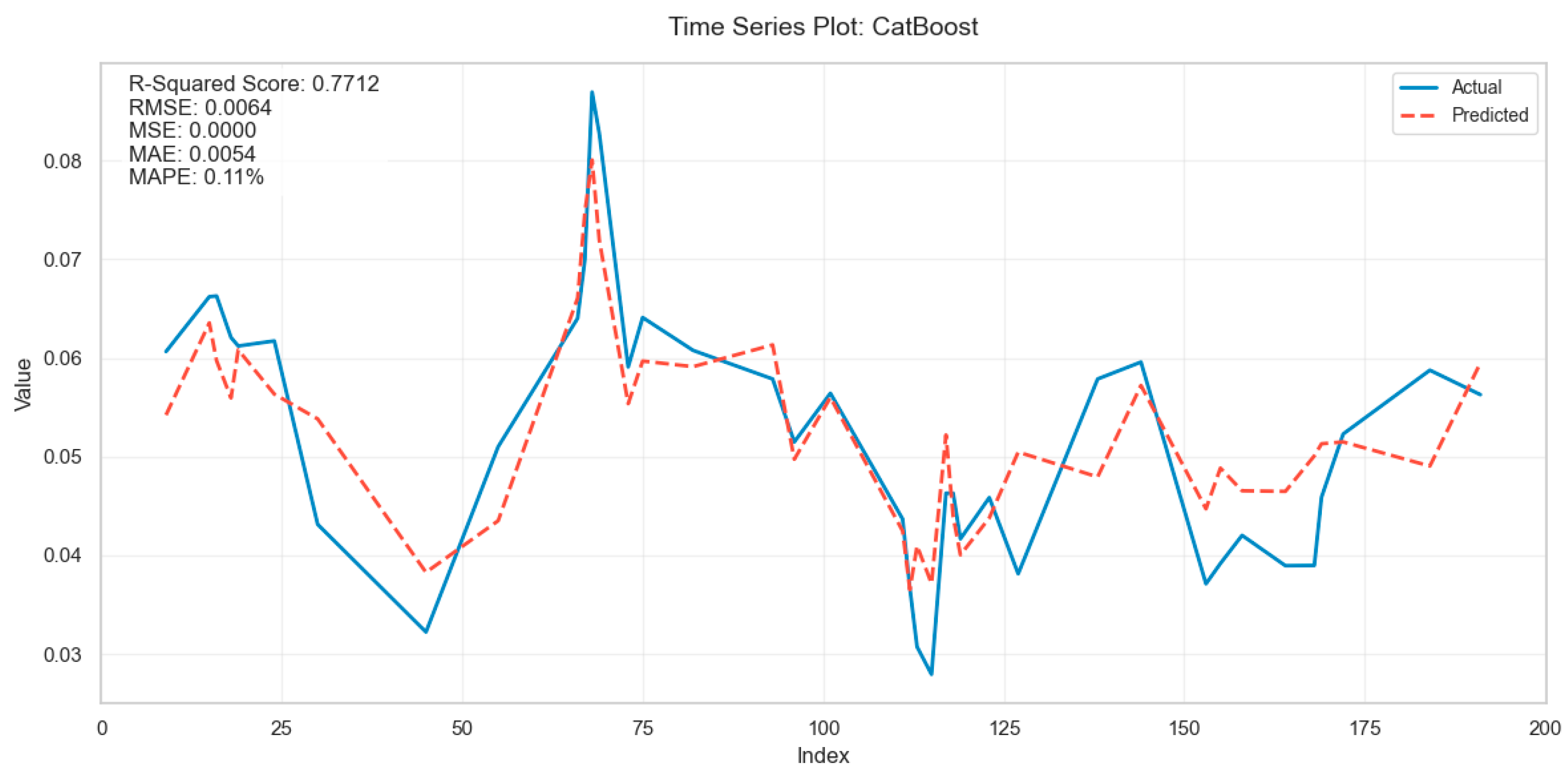
This study presents a predictive framework for membrane fouling in full-scale MBR systems by integrating AI-driven feature engineering and explainable AI (XAI). The developed predictive framework is intended for direct application in real MBR plants. By utilizing parameters routinely measured in operational settings and incorporating robust interpretable AI models, the framework supports proactive fouling management and operational decision making. By refining the target parameter to specific flux (Flux/TMP) and incorporating COD removal efficiency as a biological performance indicator, the model captures the dynamic interplay between operational parameters and fouling behavior. The application of moving average techniques further enhanced temporal feature representation, addressing the cumulative effects of fouling progression. Among tested models, CatBoost demonstrated superior predictive accuracy, outperforming traditional statistical and machine learning approaches.

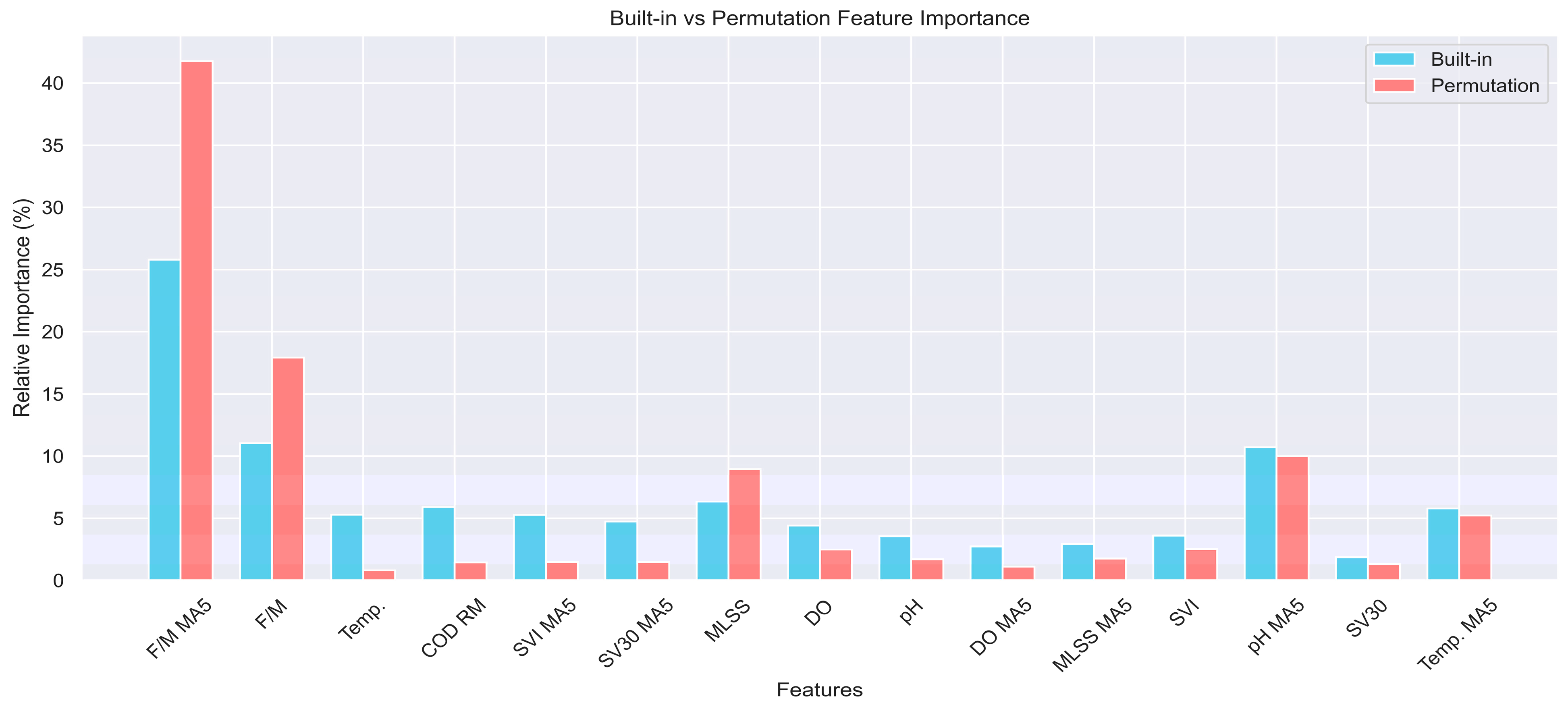
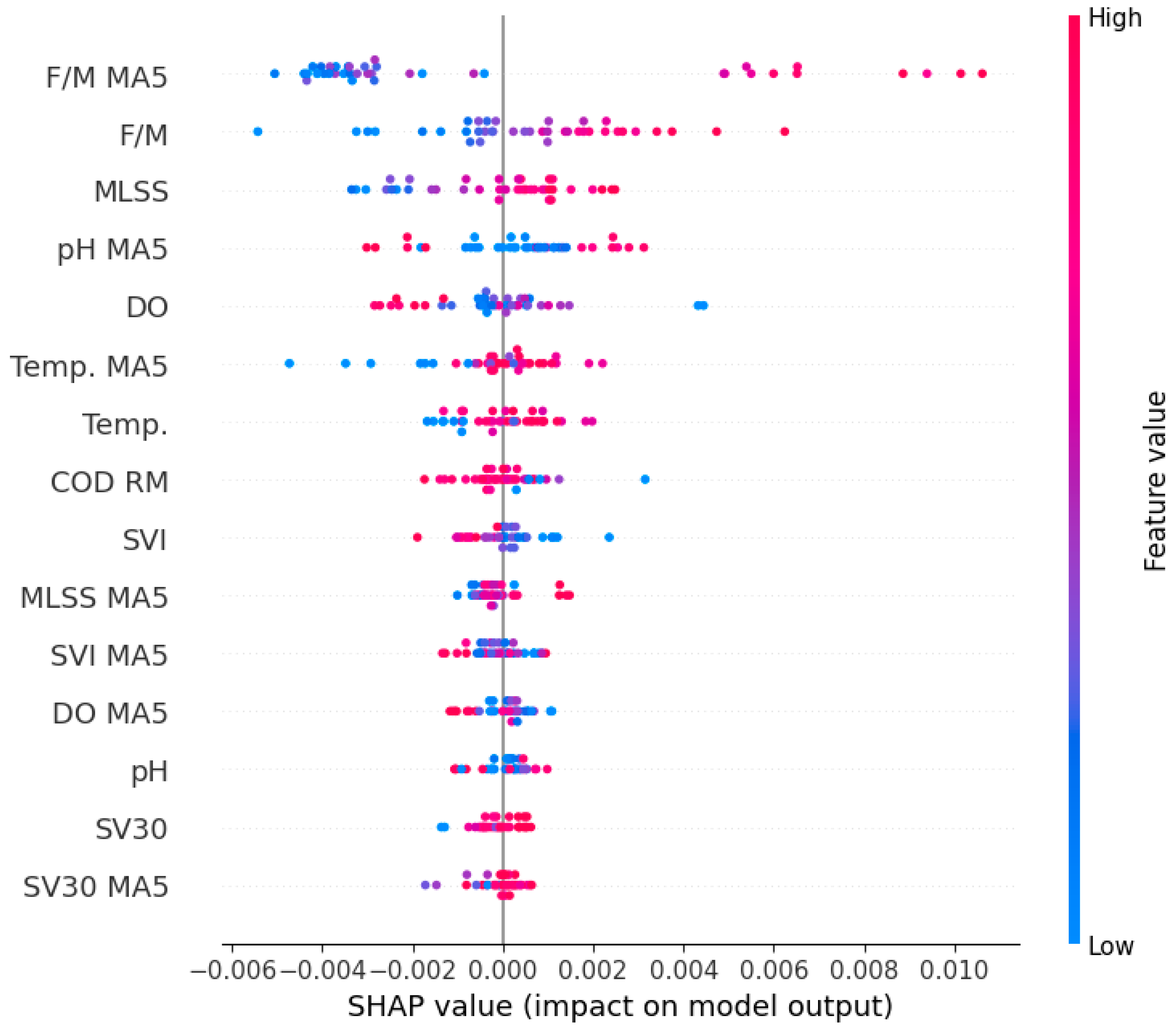
XAI techniques revealed critical insights into fouling mechanisms, identifying F/M ratio and MLSSs as dominant factors influencing fouling dynamics. These findings underscore the importance of real-time monitoring and adaptive control strategies, such as optimizing organic loading and biomass concentration, to mitigate fouling risks. While the proposed framework is not intended to replace physics-based control models, its predictive capability and interpretability provide critical decision support inputs for optimizing maintenance schedules and informing adaptive control strategies in full-scale MBR operations. The framework’s validation using real-world data from an operational MBR highlights its practical applicability under non-ideal conditions. The framework synergizes with physics-based models (e.g., biofilm dynamics simulations) by providing data-driven refinements to fouling predictions, while its compatibility with low-cost sensors bridges gaps in traditional monitoring tools. This integration enables adaptive control strategies that dynamically adjust operational parameters (e.g., aeration intensity, sludge retention) based on real-time fouling risk assessment. However, the relatively small dataset limits the generalizability of the model. Future studies should validate the framework using larger and more diverse datasets to enhance robustness and applicability across different MBR configurations.

This work demonstrates that prediction and interpretation of fouling behavior is achievable even under suboptimal data conditions, providing a critical bridge between academic research and industrial practice. In addition, this work bridges the gap between complex AI models and operational interpretability, offering a robust tool for proactive membrane management. Future research should prioritize the integration of these AI-based models with sensor networks and adaptive control systems, thereby enabling the dynamic optimization of operational parameters such as aeration, sludge retention, and filtration protocols in real time. Such efforts are expected to enhance the overall efficiency of MBR processes, reduce energy consumption, and contribute to the extension of membrane lifespan. The methodology’s adaptability also holds promise for broader applications in membrane-based processes, including desalination and industrial wastewater treatment, fostering sustainable advancements in water resource management. The core principles of this framework—dynamic target parameters (e.g., specific flux), temporal feature engineering, and XAI interpretability—are transferable to other membrane processes like reverse osmosis (RO). For instance, RO fouling is similarly time-dependent and influenced by operational fluctuations (e.g., pressure, flux variations). Adaptations would require domain-specific adjustments (e.g., incorporating scaling indices for mineral fouling), but the methodology’s foundation in handling noisy real-world data and capturing cumulative effects remains broadly applicable across membrane technologies. Future work will focus on integrating the model with online monitoring systems for real-time prediction and adaptive control in full-scale facilities.