Abstract
Aerosol uniformity in the mixing chamber is one of the key factors in evaluating performance of aerosol samplers and accuracy of aerosol monitors which could output the direct reading of particle size or concentration. For obtaining high uniformity and a stable test aerosol sample during evaluation, a portable mixing chamber, where the sample and clean air were dual-vortex turbulent mixed, was designed. By using computational fluid dynamics (CFD), particle motion within the mixing chamber was illustrated or explained. By adjusting critical structure parameters of chamber such as height and diameter, the flow field structure was optimized to improve particle mixing characteristics. Accordingly, a novel portable aerosol mixing chamber with length and inner diameter of 0.7 m and 60 mm was developed. Through a combination of simulations and experiments, the operating conditions, including working flow rate, ratio of carrier/dilution clean air, and mixture duration, were studied. Finally, by using the optimized parameters, a mixing chamber with high spatial uniformity where variation is less than 4% was obtained for aerosol particles ranging from 0.3 μm to 10 μm. Based on this chamber, a standardized testing platform was established to verify the sampling efficiency of aerosol samplers with high flow rate (28.3 L·min−1). The obtained results were consistent with the reference values in the sampler’s manual, confirming the reliability of the evaluation system. The testing platform developed in this study can provide test aerosol particles ranging from sub-micrometers to micrometers and has significant engineering applications, such as atmospheric pollution monitoring and occupational health assessment.
1. Introduction
Aerosols are liquid or solid particles suspended in a gas medium. Based on their sources, aerosols in the environment are categorized into natural origin [1,2,3,4,5] and anthropogenic origin [6,7,8,9,10]. Aerosols have a significant impact on the climate [11,12,13] by reflecting solar radiation or absorbing heat and altering the Earth’s energy balance. Also, they can act as cloud condensation nuclei to change cloud properties, lifetimes, and precipitation efficiency. At the same time, aerosols present a high health risk [14,15,16,17]. Particles with an aerodynamic diameter ≤ 2.5 µm (PM2.5) can enter the lungs and harm the respiratory system. Bioaerosols such as pollen can interfere with the immune system. In addition, aerosols affect the Earth’s ecosystems [18,19]. Aerosols containing sulfates and nitrates can form acid rain, damaging forests, lakes, and river ecosystems.
Consequently, extensive research has been conducted on aerosols. Laboratory investigations primarily employ experimental measurement techniques and numerical simulation approaches to study aerosol flows. Experimental methodologies encompass non-intrusive optical diagnostics, including Phase Doppler Particle Analyzers (PDPA) [20,21] and Particle Image Velocimetry (PIV) [22], alongside in-situ sampling techniques such as Scanning Mobility Particle Sizers (SMPS) [23] and impaction samplers [24]. Widely adopted numerical methods [25,26,27,28] feature Euler–Lagrangian frameworks utilizing Discrete Phase Models (DPM) and Discrete Element Methods (DEM), Euler–Euler frameworks implementing Multi-Fluid Models (MFM), and high-fidelity turbulence resolution techniques including Direct Numerical Simulation (DNS) and Large Eddy Simulation (LES). These combined approaches enable quantitative characterization of aerosol concentration, particle size distribution, and velocity fields, thereby establishing fundamental insights into aerosol behavior and transport mechanisms.
To respond to climate change and safeguard public health, regular monitoring of ambient aerosols is required. There are several kinds of instruments for monitoring ambient aerosols, including aerosol samplers [29], real-time monitors [30], composition analyzers [31], and remote sensing devices [32]. These instruments can monitor common aerosols in the environment, typically ranging from 0.1 to 20 μm. Due to different operating principles and techniques employed for those instruments, performance differences might occur and therefore calibration is required to ensure the accuracy of these instruments’ detection results.
Generally, to calibrate those above instruments, test aerosols with a single component and fixed concentration should be generated in the lab [33,34]. To obtain test aerosols with suitable particle size and uniform concentration, choosing the appropriate methods for aerosol generation and mixture is a critical step. Aerosol generators can be classified into different types [35,36,37,38] according to their working principles, including pneumatic atomization, ultrasonic atomization, vibrating orifice, dust or powder generators, condensation growth, etc. The suitable aerosol generator should be selected based on the characteristics of the target test aerosol such as particle size, concentration, and dispersion. Commonly used aerosol-mixing devices are mainly wind tunnels and aerosol mixing chambers. Wind tunnels [39,40,41] are devices designed to study the movement, diffusion, and settling of particles in a controlled airflow environment. Although wind tunnels can generate high-uniformity aerosols at different wind speeds (0.5–10 m/s), generally, more space and expense are needed. By contrast, aerosol mixing chambers [42,43] could provide homogeneous aerosols rapidly, with lower operating costs and a smaller footprint than wind tunnels.
Horender conducted extensive research on aerosol mixing chambers in 2019 [43]; they designed a chamber with a total length of four meters and an inner diameter of 16.4 cm. It operates at a flow rate of 180 L·min−1 and can mix particles ranging from 100 nm to 10 μm. Experiments showed that it achieves spatial uniformity better than 6% for 3 μm polystyrene latex (PSL) particles. In 2021 [44], they reduced the chamber’s height to 2.1 m and tested the particle mixing effect using sodium chloride (50 nm) and ISO A2 dust (micron-level polydisperse particles), concluding that the chamber’s spatial uniformity was within ±3%. This optimized chamber was used for calibrating PM2.5 and PM10 sensors [45] and mass spectrometers [46]. To improve the portability of the calibration system, in 2022 [42], they developed a portable aerosol mixing chamber with a height of 0.8 m and airstream flowrate of 60 L·min−1; by using this chamber, homogeneous aerosol samples (a spatial uniformity of less than 4%) with particles less than 5 μm could be obtained, and the laser scattering monitors with less than 5L/min sampling rate could be calibrated. In this research, techniques of particle mixing by using a chamber have been developed and great progress has been achieved. However, the performance of instruments for aerosols in the large particle size range, typically up to 10 μm or even larger, needs to be evaluated and calibrated on site. Moreover, due to their large sampling flow rate (typically up to 28.3 L/min), it is necessary to develop portable particle mixing chambers or calibration systems which have good mixing effects on large particles and can be applied to high flow samplers/monitors. For example, it has been shown that the particle counting efficiency of OPC or OPS is not consistent across their full particle size range, and since many OPCs are used for online monitoring of cleanliness, establishing a portable particle calibration system for online calibration of such instruments is particularly important. Meanwhile, the Andersen sampler is a multi-stage, cascade-type solid impaction-based sampler commonly used for the graded collection of airborne particles of different sizes, which is used as a standard sampling method in many fields. It is an effective way to evaluate and calibrate sampling efficiency for each stage to ensure the reliability of measurement results.
For aerosol mixing chambers, an effective way to enhance its portability is by reducing the volume and airstream working flowrate; however, this can result in a reduced mixing effect on larger particles. The aerosol mixing chamber primarily relies on the turbulent principles for particle mixing [42]. When particle size increases, the particle mass increases with diameter, leading to enhanced inertial effects—manifested as a greater resistance to changes in the state of motion induced by the fluid. Within a fixed turbulence field (constant k, ε), larger particles exhibit extended relaxation times due to increased size, allowing inertia to govern their motion. This makes such particles more likely to maintain their direct initial movement. Consequently, these particles tend to mainly distribute directly beneath the particle inlet (at the center of the sampling plane), thereby leading to uneven distribution of particles across the sampling plane.
To achieve an optimal mixing effect in chamber for particles up to 10 μm, and further for calibration of instruments with large sampling flowrate, this study proposes a mechanism for dual-vortex turbulent mixing. By combining CFD simulations with experiments, the structure and operating conditions of the mixing chamber were optimized. The aerosol mixing chamber, with a height of 0.7 m, achieved a great mixing effect of particles ranging from 0.3 to 15 μm (spatial uniformity better than 4%). The chamber was applied to evaluate the performance of an Anderson eight-stage cascade impactor sampler. The designed aerosol mixing chamber can calibrate the performance of different aerosol instruments, providing stable test aerosols for fundamental research.
2. Simulation Approach
2.1. 3D Model
The geometric model of the aerosol mixing chamber with a diameter of 59 mm and total length of 700 mm is shown in Figure 1a. The top section contains one aerosol inlet pipe and three carrier gas inlet pipes; three dilution gas inlet pipes located at approximately 160 mm below the top are arranged at 60° inclination angles, evenly distributed along the chamber’s side walls. An exhaust outlet with a diameter of 59 mm is positioned 80 mm above the chamber’s base.
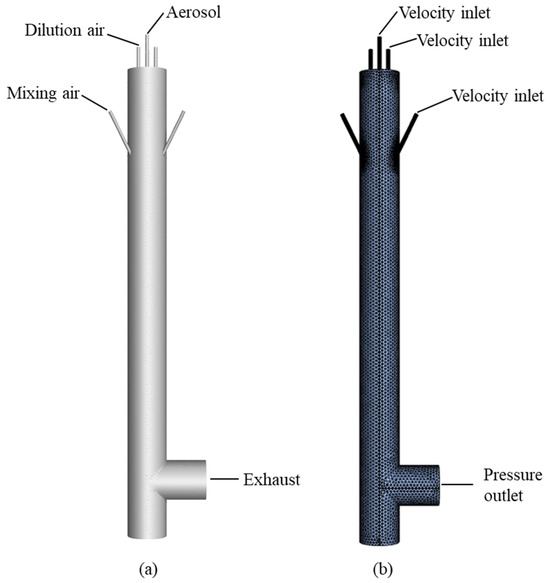
Figure 1.
Design of the aerosol mixing chamber. (a) Geometric model, (b) grid strategy.
In this study, tetrahedral elements were employed for model discretization, as shown in Figure 1b. Considering the significant impact of mesh density on computational accuracy and convergence, a grid independence verification was conducted across four mesh configurations: 367,664, 640,101, 962,381, and 1,177,334 elements. As detailed in Table 1, the mass flow rate on the sampling plane stabilized when using 640,101 elements with a relative error (RE) below 0.5%. Consequently, this mesh configuration was selected for subsequent CFD simulations to effectively balance computational accuracy with resource efficiency.

Table 1.
Mass flow rate of sampling planes at different mesh number.
2.2. Turbulence Modeling
The computational domain predominantly featured laminar flow except at the gas and aerosol inlets where localized turbulence developed. The SST k-ω model was adopted for its enhanced capability to capture adverse pressure-gradient-induced separation, combined accuracy from integrating k-ε and k-ω formulations, and advantages in computational stability, cost-effectiveness, and convergence behavior.
The SST k-ω transport equations are as follows:
where and denote the effective diffusivity of turbulent kinetic energy (k) and dissipation rate (ω); and denote the production of k and ; and denote the dissipation of k and .
Additionally, in the downstream section of the dilution gas inlet, the velocity of both gases and particles gradually decreases. The flow transitions from turbulent to laminar, with the flow behavior and particle distribution stabilizing. This results in uniform particle distribution at the sampling plane, preventing discrepancies in particle concentration during simultaneous sampling by multiple instruments.
2.3. Discrete Phase Model (DPM)
This study investigates the flow and mixing processes of particles in the aerosol mixing chamber. Since the particle volume is significantly smaller than that of the gas, the Discrete Phase Model (DPM) is employed to calculate the trajectories of particles within the flow field. In the DPM framework, the Eulerian approach is used to describe the continuous phase, while the Lagrangian method is adopted for the discrete phase. The mathematical model governing particle trajectories is formulated as follows:
The first term on the right-hand side represents the drag force, where denotes the gas velocity (m·s−1) and denotes the particle velocity (m·s−1). The second term represents the gravitational force, where denotes the gravitational acceleration (m·s−2), denotes the particle density (kg·m−3), and denotes the gas density (kg·m−3). The third term, F, corresponds to additional forces acting on the particle, including the added mass force and the Saffman lift force.
The expression for is formulated as follows:
where denotes the air viscosity (Pa·s−1), denotes the particle density (kg·m−3), denotes the particle diameter (m), denotes the drag coefficient, and Re denotes the relative Reynolds number.
The parameters related to DPM set in the experiment are shown in Table 2. The test aerosol used in the experiment was polystyrene, which has a density of 1050 kg·m−3 and is available in five particle sizes: (0.3, 1, 5, 10, and 15) μm. The simulation parameters were set to be consistent with these experimental values. The particle mass flow rate was set to (2.47 × 10⁻¹⁸–3.09 × 10⁻¹⁰) kg·s−1. This range was determined by converting the particle number concentration to mass flow rate. Given a number concentration of 1 × 10⁴ #·min−1 (consistent with experimental conditions) and particle sizes ranging from 0.3 to 15 μm, the corresponding mass flow rate falls within the range of (2.473 × 10⁻¹⁸–3.091 × 10⁻¹⁰) kg·s−1. The particle release time was set to (1–60) s to reduce computational demands, as the total simulation time was configured for a maximum of 60 s.
Table 2.
DPM parameters.
2.4. Boundary Condition
The boundary condition is set to three velocity inlets and one pressure outlet, and the specific parameters are shown in Table 3.
Table 3.
Boundary condition parameters.
2.5. Solver Setting
The solver is set up with the SIMPLEC algorithm for pressure–velocity coupling, PRESTO! for pressure discretization, and second-order upwind scheme for momentum, turbulent kinetic energy, and specific dissipation rate discretization. The solution is carried out via a transient solver with a time step of 0.005 s and a total computation time of 30 s, with convergence criteria of residuals below 10−4 for all equations.
3. Experimental Methods
3.1. Equipment
There were three components in our experimental equipment, i.e., an aerosol generation system, an aerosol mixing chamber, and an aerosol detection system, as illustrated in Figure 2. In this study, test aerosols with particle sizes ranging from 0.3 to 10 μm were generated using an atomizer generator (Kanomax, Suita, Japan) and a dust generator (Beijing Huironghe, Beijing, China) to produce aerosols in the 0.3–6 μm and 6–10 μm ranges, respectively. The atomizer generator obtains aerosol samples by impacting a suspension of polystyrene with airflow to produce droplets, which are subsequently dried into solid particles. This method could achieve polystyrene aerosol samples with high concentrations and exhibits high efficiency for generating small-sized polystyrene particles. The dust generator disperses solid samples into the air by adjusting vibration frequency, and the samples are then diluted and mixed with airflow to form aerosols. This demonstrates higher efficiency for generating large-sized particles.
Figure 2.
Aerosol homogeneity testing and instrument calibration equipment.
The aerosol mixing chamber was custom-made for this study. It was modeled in SolidWorks 2022 software and subsequently manufactured. The aerosol detection system consists of an isokinetic sampling device and particle detection instruments. The isokinetic sampling probe, made of stainless steel, incorporates two nozzles with different inner diameters to enable sampling for instruments operating at varying flow rates. Depending on experimental objectives, either a real time instrument (e.g., an optical particle counter operating at 2.83 L·min−1) or a sampler (e.g., an Andersen eight-stage sampler at 28.3 L·min−1) can be connected for testing.
3.2. Aerosol Concentration Uniformity Evaluation Method
The sampling plane in this study is a 59 mm diameter circular plane. To assess the uniformity of aerosol concentration across this sampling plane, five monitoring points were selected: the plane’s center and four additional positions at radial distances of 8 mm, 13 mm, 18 mm, and 23 mm from the center. These points are labeled as m0, m1, m2, m3, and m4 (Figure 3).
Figure 3.
Locations of five sampling points on the sampling plane.
During the CFD simulation, aerosol concentrations at each sampling point were recorded at 0.1 s intervals. Following the simulation, the cumulative aerosol number concentration over a 30 s period was calculated. The simulation data were used to determine the relative standard deviation (RSD) of aerosol concentrations across the sampling plane. In the experimental setup, two optical particle counters (OPCs) were utilized to measure aerosol concentrations at those five points: one positioned at point m0 and the other sequentially at points m1 to m4. Measurements were performed over a 30 s period with three replicate trials under identical conditions. After the experiments, aerosol concentrations at all sampling points were normalized to the reference concentration at point m0. The RSD of cumulative aerosol concentrations across the plane was calculated to evaluate uniformity.
3.3. Andersen Sampler Sampling Efficiency Evaluation Method
The physical sampling efficiency of the Andersen sampler (Model TE-20-800; Tisch Environmental, Inc., Cleves, OH, USA) was evaluated experimentally using the upstream-downstream method. Based on its operational range, 18 kinds of monodisperse polystyrene particles ranging from 0.3 to 12 μm were selected for the study. This method measures aerosol concentrations upstream and downstream of the sampler and quantifies the particles collected by the sampler.
The experimental procedure comprised three key steps: (1) generating aerosol particles, (2) homogenizing the aerosol within a mixing chamber, and (3) collecting samples via an isokinetic sampling head attached to the chamber’s base. The sampling system was integrated with both an optical particle counter (OPC) and an Andersen sampler. By alternating the valves, the OPC sequentially measured aerosol concentrations upstream and downstream of the Andersen sampler. All experiments were conducted in triplicate under identical conditions.
To evaluate the sampling efficiency of the eight-stage Andersen sampler, the efficiency of each stage was measured individually. During the initial testing, the entire sampler was connected to the system, and then each stage was removed step-by-step to assess the efficiency of the corresponding stage. There is a nominal flow rate of 28.3 L·min−1 for the Andersen sampler, and pressure drop might be changed after each stage removal, which could cause the variation of sampling flow rate. For maintaining the required flow rate, a flowmeter and an orifice valve were used to adjust and monitor the pumped flow rate.
4. Results and Discussion
4.1. Particle Motion Process Analysis
The pathlines of particles entering the mixing chamber at different times are illustrated in Figure 4a. The figure shows pathlines at different time points from 0.8 s to 20 s. The pathlines after 5 s are largely consistent, indicating that the flow has stabilized after 5 s. The particle motion process is as follows: after entering the chamber, the particles initially follow the downward airflow direction. Under the influence of three high-speed carrier gas streams positioned at the upper section, three vortices are generated (Figure 4b). The formation of vortices is caused by fluid curling induced by the velocity difference between the aerosol inlet flow (2.4 m·s−1) and the carrier gas flow (11.3 m·s−1). Additionally, since the device features three carrier gas inlets, three vortices are thus formed, which drive particle dispersion radially outward from the central region to the peripheral areas. Part of the particles become entrained in upward recirculating flows within these vortices, while others continue their downward migration. Subsequently, three additional high-speed dilution gases positioned at the chamber’s lateral walls induce other vortices, further enhancing particle homogenization through dynamic mixing mechanisms. Following this secondary dispersion phase, the particles continue their downward trajectory under controlled airflow conditions. This multistage process ultimately achieves uniform aerosol distribution across the sampling plane, ensuring spatial homogeneity of particle concentrations in the measurements.
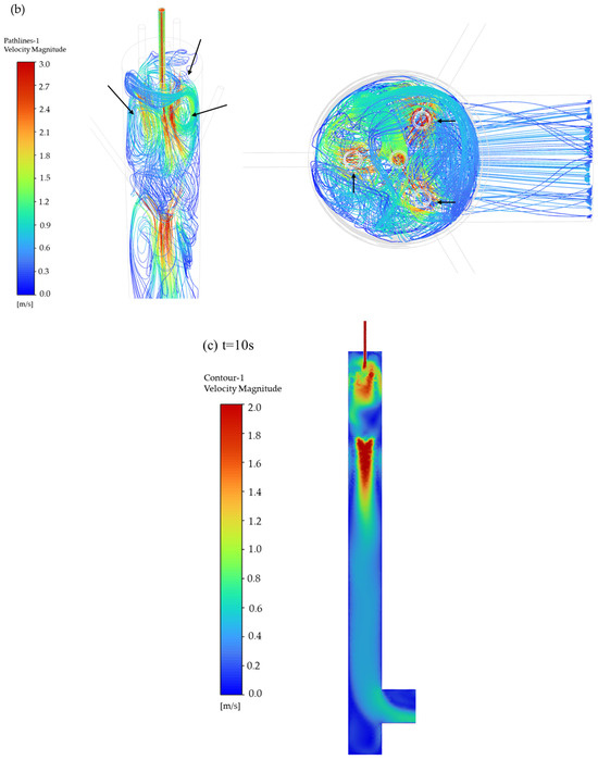
Figure 4.
Particle movement in the aerosol mixing chamber. (a) Pathlines, (b) three vortex pathlines, (c) velocity distribution contour (t = 10 s).
The formation of vortices within the mixing chamber is attributed to the difference in gas velocity. Figure 4c displays the velocity distribution contour of the internal z = 0 cross section. As gas enters the chamber from the high-speed pipeline (11.4 m·s−1), the sudden expansion of flow area causes jet expansion, where the carrier gas and the dilution gas decelerate progressively from 11.4 m·s−1 to 1.2 m·s−1. Concurrently, the aerosol velocity decreases from 2.4 m·s−1 to 1.2 m·s−1. The velocity disparity between the aerosol and carrier gas generates a localized pressure gradient, initiating vortex formation that enhances particle mixing. Subsequently, the downward-moving aerosol interacts with the dilution gas. This interaction creates shear forces due to both velocity differences and opposing flow directions, further amplifying vortical structures. The turbulence ensures continuous particle redistribution.
Vortex formation facilitates thorough particle mixing in the chamber, while high-velocity outflow initially maintains turbulent conditions with unstable flow patterns. As the flow progresses downward, velocity gradually diminishes, enabling a hydrodynamic transition from turbulent to laminar regimes. Figure 5 presents velocity vector diagrams of specific planes at t = 10 s (y = 200, 300, 400, 500 mm). By monitoring particle pathlines and velocity contours, it was observed that the mixing chamber achieves a quasi-steady state after t = 5 s. Hence, the velocity vector plot at t = 10 s serves as a representative illustration of the flow field. With decreasing height, fluid motion becomes progressively aligned, evolving from being multidirectional in upper regions to uniformly vertical at lower sections. The Reynolds number decreases from 3800 on the gas inlet to 400 on the sampling plane. Additionally, the radial velocity profile monitored at the sampling plane follows the Hagen–Poiseuille distribution (Appendix A). It demonstrates that the height-dependent flow transformation demonstrates the systematic transition from turbulent motion to laminar behavior, ensuring uniform particle distribution on the sampling plane.
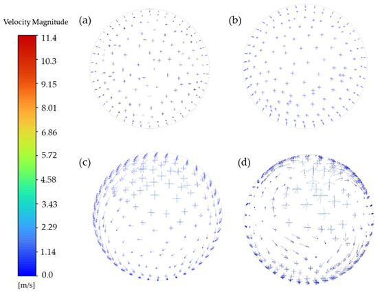
Figure 5.
Velocity vectors for different heights (Arrows indicates the direction of the speed). (a) y = 200 mm, (b) y = 300 mm, (c) y = 400 mm, (d) y = 500 mm.
4.2. Structural Optimization of the Aerosol Mixing Chamber
This study conducted systematic research on the structural optimization of the aerosol mixing chamber through CFD simulations. By establishing a three-dimensional transient Discrete Phase Model, this study comprehensively investigated the influence of key structural parameters (including the main chamber height and aerosol inlet diameter) on particle distribution uniformity and mixing efficiency. It is particularly noteworthy that, regarding inlet pipeline configuration, this work adopted a “1 + 3 + 3” multi-channel structure (i.e., one aerosol inlet, three carrier gas inlets, and three dilution gas inlets) based on experimental data from prior studies on aerosol mixing chambers. This innovative configuration successfully achieved the compact device design goal while ensuring efficient particle diffusion.
4.2.1. Height
The vertical dimension of mixing chambers constitutes a critical design parameter that directly impacts system performance. Excessive height leads to unnecessary volume expansion and footprint, while an insufficient vertical dimension compromises the particle mixing effects. This study systematically evaluated the aerosol uniformity of different heights (0.32 m, 0.51 m, 0.70 m, and 0.89 m).
Figure 6 presents violin plots illustrating aerosol concentration distributions at multiple monitoring points, constructed from CFD simulation data recorded at 0.1 s intervals. It demonstrates that increased mixing chamber height leads to reduced concentration variability across measurement locations. Table 4 quantifies this trend through RSD analysis of 30 s cumulative concentrations. Notably, the RSD decreases from 17.86% at 0.32 m to 2.98% at 0.70 m, representing a 6-fold reduction in RSD. This parameter plateaus beyond 0.70 m, showing negligible change (2.98% to 3.01%) when height increases further to 0.89 m.
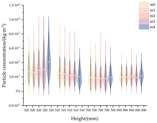
Figure 6.
Violin plots of aerosol concentration based on different aerosol mixing chamber heights.
Table 4.
RSD of aerosol concentration based on different aerosol mixing chamber heights.
This phenomenon fundamentally is governed by particle dynamics within the system. Upon entering the aerosol mixing chamber, particles undergo two turbulent cycles before entering the main conduit, where diminished flow velocity and reduced Re facilitate hydrodynamic transition to the laminar regime. In this stabilized laminar state, fluid layers maintain parallel trajectories without cross-mixing, enabling uniform aerosol distribution for sampling or detection. Reduced chamber height induces incomplete flow transformation, maintaining particles in a transitional regime where residual turbulence disrupts uniform distribution. The simulations demonstrate that 0.70 m chamber height leads to full laminar conversion, meeting homogeneity requirements (RSD < 3%). However, increasing height beyond 0.70 m shows negligible improvement in particle uniformity. This approach unnecessarily increases equipment footprint. Therefore, subsequent investigations adopted the optimized 0.70 m height, balancing operational efficiency with spatial efficiency in aerosol processing systems.
4.2.2. Diameter of Aerosol Inlet Pipes
Under constant flow rate conditions, variations in pipe diameter significantly affect both fluid and particle velocities. The modification of aerosol inlet diameter in the homogenization chamber alters aerosol flow velocity. This study investigates particle mixing efficiency under a fixed aerosol flow rate of 2.83 L·min−1 through the CFD simulations, comparing three designed inlet diameters: 2.5 mm, 3.75 mm, and 5 mm.
Figure 7 displays violin plots of aerosol concentration monitored at five positions with 0.1 s intervals under three inlet diameters. For 2.5 mm and 3.75 mm configurations, significant median discrepancies and broader spreads were observed between monitoring positions, whereas the 5 mm configuration exhibited uniform medians with tightly clustered distributions. Further statistical quantification of 30 s cumulative concentrations demonstrated critical differences in spatial homogeneity: RSD exceeded 7% for both 2.5 mm (17.32%) and 3.75 mm (7.21%), while the 5 mm design achieved optimal uniformity (RSD = 2.98%, Table 5).
Figure 7.
Violin plots of aerosol concentration based on different aerosol inlet diameters.
Table 5.
RSD of aerosol concentration based on different aerosol inlet diameters.
This phenomenon is related to aerosol flow velocity. As the tube diameter increases, particle velocity gradually decreases. At a 2.5 mm inlet diameter, the aerosol exhibits a flow velocity of 8.5 m·s−1, which is equivalent to the dilution gas velocity. For a 3.75 mm inlet diameter, the aerosol velocity decreases to 4.25 m·s−1 (50% of the gas velocity). When the diameter is set to 5 mm, the aerosol velocity stabilizes at 2.4 m·s−1. Based on the calculations of vorticity and turbulence intensity at the plane (P1) 20 mm below the aerosol inlet (Table 6), it is evident that as the pipe diameter increases, both vorticity magnitude and fluid rotational intensity rise, while turbulence intensity also increases. The velocity difference induces large-scale vortices and high turbulence intensity, which significantly enhances interphase momentum exchange and homogenizes the mixture. This velocity-gradient-driven turbulence mechanism justifies the selection of 5mm diameter for subsequent system optimization.
Table 6.
Vorticity and turbulence intensity of P1.
4.3. Operational Parameters of the Aerosol Mixing Chamber
4.3.1. Flow Rate
The working flow rate of the aerosol mixing chamber is a critical operational parameter, as it directly influences the velocity distribution of internal airflow and the motion of particles. When utilizing the mixing chamber, the working flow rates of sampling or detection instruments connected downstream may vary, with commonly used instruments operating in the range from 2.83 L·min−1 to 28.3 L·min−1. Therefore, to explore the suitable operational flow rate range for the mixing chamber designed in this study, simulations and experiments were systematically conducted at flow rates of 15 L·min−1, 30 L·min−1, 45 L·min−1, and 60 L·min−1.
Figure 8 presents violin plots of aerosol concentrations at five monitoring points under different flow rates. The results reveal that as the flow rate decreases, the monitored aerosol concentrations progressively increase, with concentrations at 15 L·min−1 and 60 L·min−1 differing by approximately one order of magnitude. This trend is attributed to particle motion dynamics: reduced flow rates lower the velocities of both fluid and particles, extending the residence time within the chamber and thereby enhancing aerosol accumulation.
Figure 8.
Violin plots of aerosol concentration at different workflow rate.
Table 7 displays the 30 s cumulative aerosol concentrations at five monitoring points and the RSD of aerosol concentrations across varying flow rates. As the flow rate decreases, the RSD progressively increases, with values below 2.5% at 30–60 L·min−1 and exceeding 6% at 15 L·min−1, indicating superior aerosol homogenization within the 30–60 L·min−1 range. While experimental results align with CFD simulation trends, higher RSD values in physical tests are attributed to simplifications in the numerical modeling framework.
Table 7.
RSD of aerosol concentration at different workflow rates.
This phenomenon is associated with the vortical motions. As illustrated in Figure 9, the aerosol undergoes two types of vortices formations induced by carrier gas and dilution gas interactions to achieve particle homogenization. Particle pathline diagrams at 30–60 L·min−1 demonstrate the complete two types of vortex cycles. As indicated by the maximum vorticity magnitude calculations (Table 8) on the plane 20 mm downstream from the aerosol inlet pipe, the maximum vorticity magnitude increases with higher flow rates. This demonstrates intensified vortex rotation, enhancing particle dispersion from below the inlet throughout the mixing chamber. To achieve a better mixing effect, it is recommended to use this equipment at an operating flow rate of 30–60 L·min−1.
Figure 9.
Particle pathlines at different flow rates. (a) 15 L·min−1, (b) 30 L·min−1, (c) 45 L·min−1, (d) 60 L·min−1.
Table 8.
The maximum vorticity magnitude on plane P1 at different flow rates.
4.3.2. Carrier/Dilution Gas Ratio
In this study, the gas entering the mixing chamber is primarily categorized into two types: carrier gas and dilution gas. Both collectively function to form vortices with the aerosol, enhancing particle uniformity. Additionally, the carrier gas provides the driving force for the vertically downward motion, while the dilution gas regulates aerosol concentration and flow rate. This section investigates the influence of the carrier-to-dilution gas ratio at a total flow rate of 60 L·min−1 on particle mixing effectiveness.
The carrier/dilution gas ratios were set as 0.5, 1, and 2. Figure 10 displays violin plots of aerosol concentrations recorded every 0.1 s across five sampling sites. As shown, the median aerosol concentrations at all sites remain largely consistent, with minimal impact from changes in the carrier/dilution gas ratio. Table 9 presents the RSD for simulated and experimental aerosol concentrations on the plane at different carrier/dilution gas ratios. It reveals that particle uniformity is optimal at the ratio of 1, though particle distribution remains relatively uniform at other ratios. This factor exhibits limited influence on particle mixing effectiveness.
Figure 10.
Violin plot of aerosol concentration at different rates of carrier/dilution gas.
Table 9.
RSD of aerosol concentration at different rates of carrier/dilution gas.
The primary reason is that altering the carrier-to-diluent gas ratio does not eliminate the coexistence of these two classes of vortices but merely modifies their vorticity magnitude and rotational intensity respectively. An increase in the flow rate of either the carrier or dilution gas elevates its corresponding velocity, enlarging the vorticity magnitude while reducing the other vortex’s vorticity magnitude. Consistent vorticity magnitude is most favorable for particle mixing. However, due to the high total flow rate, uneven vortices can still mix the aerosol, with slightly reduced effectiveness compared with similar sized vortices. If the total operational flow rate is reduced, the disparity in gas flow rates may cause significant shrinkage or even disappearance of one vortex, severely compromising mixing effectiveness. Therefore, it is recommended to maintain equal carrier and dilution gas flow rates when using the mixing chamber.
4.3.3. Mixture Duration
When using an aerosol mixing chamber, the sampling duration is not fixed and commonly ranges from 0.5 to 10 min. Whether aerosol concentration uniformity is maintained across varying operating times significantly impacts research outcomes regarding sampling efficiency. This study tests aerosol concentration uniformity within the (0.5–10) min timeframe to determine if the designed mixing chamber can sustain aerosol homogeneity during extended sampling durations.
First, cumulative concentrations at five sampling sites across different time intervals were experimentally measured, with results presented in Table 10. The data demonstrate good aerosol uniformity across the plane within the 0.5–10 min sampling time. The RSD ranges from 1.45% to 2.23%, indicating that the designed system meets aerosol homogeneity requirements throughout this operational time.
Table 10.
RSD of aerosol cumulative concentration from 0.5min to 10min (experimental).
Subsequently, CFD simulations were conducted to determine the minimum time to achieve uniformly distributed aerosols by analyzing the RSD of cumulative concentrations at five planar sampling points across durations of 1 s, 2 s, 5 s, 10 s, 30 s, and 60 s. Results in Table 11 demonstrate a gradual reduction in RSD values with increasing time, reflecting progressive improvement of aerosol uniformity across the plane. A minimum sampling time of 10 s is recommended to ensure adequate particle mixing efficiency (RSD < 4%).
Table 11.
RSD of aerosol cumulative concentration uniformity in 1-60 s (CFD simulation).
This phenomenon is related to the motion of aerosols within the mixing chamber. The small-sized aerosol particles are is susceptible to airflow and external forces, resulting in unstable dynamic states. The aerosol concentration on the plane reaches approximately 2 × 10⁻⁷ kg·m−3 after 5 s (Figure 11), followed by fluctuations around this level. Increasing the sampling time reduces the impact of these fluctuations on cumulative concentration measurements. Based on experimental and simulation results, a sampling period of 10 s–10 min is recommended. Periods shorter than 10 s may degrade aerosol uniformity on the plane, while durations exceeding 10 min leads to aerosol concentration decline, with extended sampling times failing to collect additional aerosols.
Figure 11.
Time variation curve of aerosol concentration.
Additionally, after ceasing aerosol generation post-experiment, monitoring at the sampling locations revealed a two order-of-magnitude decrease in aerosol concentration within 5 s, with particles becoming undetectable after 10 s. Consequently, introducing clean gas into the mixing chamber for at least 5 s is required after the experiment to purge residual aerosols from the system.
4.3.4. Particle Diameter
The test aerosol contains particles of varying sizes, with particle size distributions ranging from submicron to micron levels. In this study, test aerosols contain particles of five different sizes (0.3 μm, 1 μm, 5 μm, 10 μm, and 15 μm). The uniformity of particles was tested through CFD simulations and experiments, and the results are shown in Table 12.
Table 12.
RSD of aerosol concentration based on different particle sizes.
From the simulation results, it can be observed that the mixing chamber designed in this study demonstrates effective aerosol mixing for particles ranging from 0.3 μm to 15 μm. Within 30 s, the RSD of cumulative concentrations at different locations on the sampling plane were all below 5%, indicating superior mixing performance for submicron and small micron-sized particles. Concurrently, as the aerosol particle size increased, the RSD of aerosol cumulative concentration gradually rose from 1.21% at 0.3 μm to 3.84% at 15 μm. This phenomenon is attributed to particle motion characteristics within the chamber. Submicron particles exhibit low inertia and are mainly influenced by drag forces and Brownian motion, and follow airflow directions with enhanced random dispersion, facilitating thorough mixing. In contrast, micro-sized particles possess greater inertia, are more affected by gravity, and resist directional changes induced by airflow, causing some to retain their initial trajectories and accumulate near the chamber’s central region, resulting in poorer dispersion compared to submicron particles.
The experiment was subsequently conducted. Since 15 μm polystyrene samples were not acquired, tests were performed using 0.3 μm, 1 μm, 5 μm, and 10 μm polystyrene particles. The experimental results demonstrated good consistency with simulation outcomes. This confirms the device’s capability to effectively mix test aerosols in the 0.3–10 μm range.
4.4. Evaluation of the Sampling Efficiency of the Andersen Sampler
Based on the designed aerosol mixing chamber and calibration system, this study investigated the physical sampling efficiency of the Andersen eight-stage sampler at 28.3 L·min−1 using the upstream-downstream method for stage-by-stage evaluation. For each stage, at least four polystyrene particles of different particle sizes were tested. The efficiency curves were fitted using a Boltzmann sigmoidal function to determine the D50 values, which were then compared with the nominal cut-off diameters specified in the sampler’s manual (Figure 12 and Table 13).
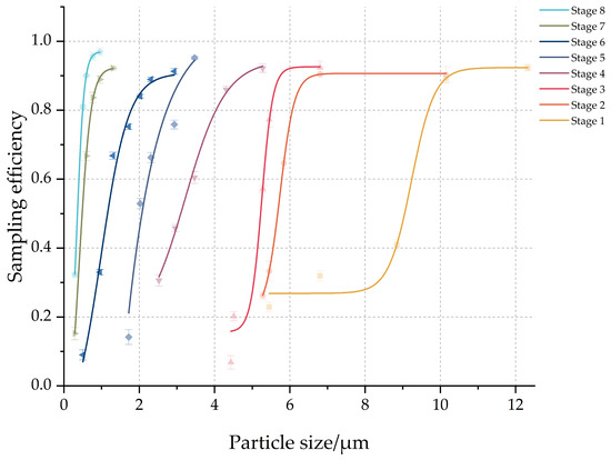
Figure 12.
Efficiency fitting curve for each level of the Anderson sampler.
Table 13.
D50 for each level of the Anderson sampler.
Analysis of the experimental results reveals that the sampling efficiency of the sampler increases with particle size. The D50 of each stage decreases as the stage number increases, which aligns with the working principle of the Andersen sampler. As a typical impaction-based sampler, the Andersen sampler separates particles through inertial impaction. Particles entering the sampler with the airflow follow the redirected gas stream toward the edges of each stage’s collection plate. Smaller particles remain entrained in the airflow and proceed to subsequent stages, while larger particles, due to their higher inertia, maintain their trajectory and are deposited on the collection substrate on the plate, leading to increased sampling efficiency for larger particles. The particle size range collected at each stage depends on the orifice diameter of the corresponding stage, as illustrated in Equation (6):
where represents the orifice diameter, is the dynamic viscosity of gas, denotes the Stokes number for particles collected at 50% sampling efficiency by the nozzle, is particle density, is the airflow velocity at the orifice, and is the Cunningham correction factor.
The D50 increases with larger orifice diameters. Therefore, as the sampler stage number increases, the orifice diameter of each stage decreases, leading to a reduction in the D50 for each subsequent stage.
A comparison between experimental results and the standard value from the manual shows good agreement, except for the relative deviations of approximately 10% observed for stages 7 and 8. This discrepancy is attributed to the particle collection mechanism of the filter membrane: for small particles (below 0.3 μm), diffusion dominates rather than inertial impaction. The D50 calculated using orifice diameter neglects particle capture due to diffusion, leading to lower experimental values for these final two stages. The aerosol sampler efficiency calibration system developed in this study is practically applicable, provides accurate evaluation results, and can adapt for calibrating other samplers.
4.5. Limitations
Compared with previous studies, this research systematically analyzes the particle motion within the mixing chamber using CFD methods, theoretically explaining how different factors influence mixing efficiency and optimizing key structural components affecting mixing uniformity. Despite these advancements, this device is primarily applicable to particles below 10 μm and operates at a minimum flow rate of 30 L·min−1. Due to the lack of 15-micron solid polystyrene standard particles, we were unable to conduct effective experimental validation. Further investigation is required for aerosol mixing involving larger particles and lower flow rates. Future studies will focus on these aspects by further reducing the device size and optimizing gas/particle inlet structures. These enhancements will expand applicability for field testing and large-particle-size evaluations.
5. Conclusions
This study developed a portable aerosol mixing chamber that achieved thorough particle mixing and stable aerosol distribution based on the dual-vortex turbulent mixing and laminar sampling principle. Through CFD simulations optimizing the structure, including height and inlet diameter, a cylindrical chamber (700 mm height, inner diameter of 59 mm) was designed. The aerosol mixing chamber provided an optimal mixing performance while simplifying the structure and reducing the footprint. Experimental investigations revealed significant correlations between gas-particle velocity differences and turbulence intensity, achieving excellent mixing effects (RSD < 4%) for particles sized 0.3–10 μm within 0.5–10 min operation. The constructed system evaluated the physical sampling efficiency of Andersen eight-stage sampler, which aligned well with the standard values in the manual.
Compared to previous studies, the CFD numerical simulations conducted in this paper using the transient method provide a more comprehensive understanding of the real-time movement and dispersion processes of particles in the mixing chamber, which facilitates understanding of the mixing processes of particles. Additionally, the “Dual Vortex Mixing Laminar Sampling” principle proposed in this study not only reduces the complexity of aerosol and carrier gas inlet pipelines but also achieves thorough mixing of large-diameter particles (exceeding 5 μm) within a compact mixing chamber. Furthermore, this equipment successfully quantitatively evaluated the sampling efficiency of the Anderson eight-stage impactor, validating the mixing effectiveness of the small-volume mixing chamber for particles larger than 5 μm, laying a foundation for on-site calibration of instruments.
In this research, the aerosol mixing chamber was designed for testing aerosol mixing in the laboratory and evaluating performance of various aerosol instruments. It achieved thorough mixing of submicron-sized and micro-sized particles within a compact design, expanding its potential applications across diverse scenarios, like on-site testing and commercial testing.
Author Contributions
Conceptualization, Z.X.; Data curation, Z.X. and Y.L.; Formal analysis, Z.X. and J.L. (Junjie Liu); Funding acquisition, J.L. (Junjie Liu), Y.L. and X.X.; Investigation, Z.X. and J.L. (Jiazhen Lu); Methodology, Z.X.; Project administration, J.L. (Junjie Liu); Supervision, J.L. (Junjie Liu); Software, Z.X. and J.L. (Jiazhen Lu); Validation, Z.X. and Y.L.; Writing—original draft, Z.X.; Writing—review and editing, J.L. (Junjie Liu), Y.L., J.L. (Jiazhen Lu) and X.X.; Software, Z.X. and J.L. (Jiazhen Lu); Validation, Z.X. and Y.L. All authors have read and agreed to the published version of the manuscript.
Funding
This research was supported by the National Key Research and Development Program of China (2023YFC3705404, 2023YFF0616400), Key Fundamental Scientific Research Projects of the National Institute of Metrology (AKYZD2308-1, AGS24306, ANL2203).
Data Availability Statement
The original contributions presented in this study are included in the article. Further inquiries can be directed to the corresponding author.
Conflicts of Interest
The authors declare no conflicts of interest.
Abbreviations
The following abbreviations are used in this manuscript:
| CFD | Computational fluid dynamics |
| DPM | Discrete Phase Model |
| OPC | Optical particle counter |
| PSL | Polystyrene latex |
| RE | Relative error |
| RSD | Relative standard deviation |
Appendix A
Figure A1.
The radial velocity profile of the sampling plane.
References
- Abbas, M.S.; Yang, Y.; Zhang, Q.; Guo, D.; Godoi, A.F.L.; Godoi, R.H.M.; Geng, H. Salt Lake Aerosol Overview: Emissions, Chemical Composition and Health Impacts under the Changing Climate. Atmosphere 2024, 15, 212. [Google Scholar] [CrossRef]
- Chaudhuri, S.; Saha, A.; Basu, S. An opinion on the multiscale nature of Covid-19 type disease spread. Curr. Opin. Colloid Interface Sci. 2021, 54, 101462. [Google Scholar] [CrossRef] [PubMed]
- Ribaric, N.L.; Vincent, C.; Jonitz, G.; Hellinger, A.; Ribaric, G. Hidden hazards of SARS-CoV-2 transmission in hospitals: A systematic review. Indoor Air 2022, 32, e12968. [Google Scholar] [CrossRef] [PubMed]
- Zhao, Y.; Zhang, Y.-L.; Sun, R. The mass-independent oxygen isotopic composition in sulfate aerosol -a useful tool to identify sulfate formation: A review. Atmos. Res. 2021, 253, 105447. [Google Scholar] [CrossRef]
- Santl-Temkiv, T.; Amato, P.; Gosewinkel, U.; Thyrhaug, R.; Charton, A.; Chicot, B.; Finster, K.; Bratbak, G.; Londahl, J. High-Flow-Rate Impinger for the Study of Concentration, Viability, Metabolic Activity, and Ice-Nucleation Activity of Airborne Bacteria. Environ. Sci. Technol. 2017, 51, 11224–11234. [Google Scholar] [CrossRef] [PubMed]
- Antonini, J.M.; McKinney, W.G.; Lee, E.G.; Afshari, A.A. Review of the physicochemical properties and associated health effects of aerosols generated during thermal spray coating processes. Toxicol. Ind. Health 2021, 37, 47–58. [Google Scholar] [CrossRef] [PubMed]
- Mahowald, N.M.; Hamilton, D.S.; Mackey, K.R.M.; Moore, J.K.; Baker, A.R.; Scanza, R.A.; Zhang, Y. Aerosol trace metal leaching and impacts on marine microorganisms. Nat. Commun. 2018, 9, 2614. [Google Scholar] [CrossRef] [PubMed]
- Malik, A.; Aggarwal, S.G. A Review on the Techniques Used and Status of Equivalent Black Carbon Measurement in Two Major Asian Countries. Asian J. Atmos. Environ. 2021, 15, 1–32. [Google Scholar] [CrossRef]
- Moteki, N. Climate-relevant properties of black carbon aerosols revealed by in situ measurements: A review. Prog. Earth Planet. Sci. 2023, 10, 12. [Google Scholar] [CrossRef]
- Li, W.; Ge, P.; Chen, M.; Tang, J.; Cao, M.; Cui, Y.; Hu, K.; Nie, D. Tracers from Biomass Burning Emissions and Identification of Biomass Burning. Atmosphere 2021, 12, 1401. [Google Scholar] [CrossRef]
- Lohmann, U. Why does knowledge of past aerosol forcing matter for future climate change? J. Geophys. Res.-Atmos. 2017, 122, 5021–5023. [Google Scholar] [CrossRef]
- Marshak, A.; Ackerman, A.; da Silva, A.M.; Eck, T.; Holben, B.; Kahn, R.; Kleidman, R.; Knobelspiesse, K.; Levy, R.; Lyapustin, A.; et al. Aerosol Properties in Cloudy Environments from Remote Sensing Observations A Review of the Current State of Knowledge. Bull. Am. Meteorol. Soc. 2021, 102, E2177–E2197. [Google Scholar] [CrossRef]
- McNeill, V.F. Atmospheric Aerosols: Clouds, Chemistry, and Climate. Annu. Rev. Chem. Biomol. Eng. 2017, 8, 427–444. [Google Scholar] [CrossRef] [PubMed]
- Clementini, M.; Raspini, M.; Barbato, L.; Bernardelli, F.; Braga, G.; Di Gioia, C.; Littarru, C.; Oreglia, F.; Brambilla, E.; Iavicoli, I.; et al. Aerosol transmission for SARS-CoV-2 in the dental practice. A review by SIdP Covid-19 task-force. Oral Dis. 2022, 28, 852–857. [Google Scholar] [CrossRef] [PubMed]
- Gorny, R.L. Microbial Aerosols: Sources, Properties, Health Effects, Exposure Assessment—A Review. Kona Powder Part. J. 2020, 37, 64–84. [Google Scholar] [CrossRef]
- Lim, C.C.; Yoon, J.; Reynolds, K.; Gerald, L.B.; Ault, A.P.; Kleo, S.; Bell, M.L. Harmful algal bloom aerosols and human health. Ebiomedicine 2023, 93, 104604. [Google Scholar] [CrossRef] [PubMed]
- Lv, J.; Gao, J.; Wu, B.; Yao, M.; Yang, Y.; Chai, T.; Li, N. Aerosol Transmission of Coronavirus and Influenza Virus of Animal Origin. Front. Vet. Sci. 2021, 8, 572012. [Google Scholar] [CrossRef] [PubMed]
- Gallisai, R.; Peters, F.; Volpe, G.; Basart, S.; Baldasano, J.M. Saharan Dust Deposition May Affect Phytoplankton Growth in the Mediterranean Sea at Ecological Time Scales. PLoS ONE 2014, 9, e110762. [Google Scholar] [CrossRef] [PubMed]
- Zhou, S.; Guo, F.; Chao, C.-Y.; Yoon, S.; Alvarez, S.L.; Shrestha, S.; Flynn Iii, J.H.; Usenko, S.; Sheesley, R.J.; Griffin, R.J. Marine Submicron Aerosols from the Gulf of Mexico: Polluted and Acidic with Rapid Production of Sulfate and Organosulfates. Environ. Sci. Technol. 2023, 57, 5149–5159. [Google Scholar] [CrossRef] [PubMed]
- Lee, S.W.; Cui, H.J.; Huang, Y.H. Particle Characteristics and Analysis Using the Laser-Based Phase Doppler Particle Analyzer (PDPA) and Statistical Method. Part. Sci. Technol. 2009, 27, 263–270. [Google Scholar] [CrossRef]
- Van den Moortel, T.; Azario, E.; Santini, R.; Tadrist, L. Experimental analysis of the gas-particle flow in a circulating fluidized bed using a phase Doppler particle analyzer. Chem. Eng. Sci. 1998, 53, 1883–1899. [Google Scholar] [CrossRef]
- Hinsch, K.D. Holographic particle image velocimetry. Meas. Sci. Technol. 2002, 13, R61–R72. [Google Scholar] [CrossRef]
- Ober, F.; Mayer, M.; Büttner, H.; Ebert, F. Aerosol measurement in low-pressure systems with standard scanning mobility particle sizers. Part. Part. Syst. Charact. 2002, 19, 229–239. [Google Scholar] [CrossRef]
- Juozaitis, A.; Willeke, K.; Grinshpun, S.A.; Donnelly, J. Impaction onto a glass slide or agar versus impingement into a liquid for the collection and recovery of airborne microorganisms. Appl. Environ. Microbiol. 1994, 60, 861–870. [Google Scholar] [CrossRef] [PubMed]
- Kaltenbach, C.; Laurien, E. CFD Simulation of aerosol particle removal by water spray in the model containment THAI. J. Aerosol Sci. 2018, 120, 62–81. [Google Scholar] [CrossRef]
- Ibarra, I.; Rodriguez-Maroto, J.J.; Rojas, E.; Sanz, D. CFD simulations to improve the aerosol tangential inlet of a Differential Mobility Analyzer. J. Aerosol Sci. 2021, 154, 105740. [Google Scholar] [CrossRef]
- Salary, R.; Lombardi, J.P.; Weerawarne, D.L.; Rao, P.K.; Poliks, M.D. A Computational Fluid Dynamics (CFD) Study of Pneumatic Atomization in Aerosol Jet Printing (AJP) Process. In Proceedings of the ASME International Mechanical Engineering Congress and Exposition (IMECE), Salt Lake City, UT, USA, 8–14 November 2019. [Google Scholar]
- Mahmoud, M.M.A.; Bahl, P.; Aquino, A.; Maclntyre, C.R.; Green, D.; Doolan, C.; de Silva, C. An infection risk model for estimating infection probability and occupancy time: A CFD approach with aerosol measurements. Build. Environ. 2025, 279, 113035. [Google Scholar] [CrossRef]
- Truyols Vives, J.; Muncunill, J.; Toledo Pons, N.; Baldovi, H.G.; Sala Llinas, E.; Mercader Barcelo, J. SARS-CoV-2 detection in bioaerosols using a liquid impinger collector and ddPCR. Indoor Air 2022, 32, e13002. [Google Scholar] [CrossRef] [PubMed]
- Lancia, A.; Gioffre, A.; Di Rita, F.; Magri, D.; D’Ovidio, M.C. Aerobiological Monitoring in an Indoor Occupational Setting Using a Real-Time Bioaerosol Sampler. Atmosphere 2023, 14, 118. [Google Scholar] [CrossRef]
- Ye, S.; Wen, Z.; Xie, K.; Gu, X.; Wang, J.; Tang, X.; Zhang, W. Online quantification of nicotine in e-cigarette aerosols by vacuum ultraviolet photoionization mass spectrometry. Anal. Methods 2024, 16, 2732–2739. [Google Scholar] [CrossRef] [PubMed]
- Choi, W.; Kang, H.; Shin, D.; Lee, H. Satellite-Based Aerosol Classification for Capital Cities in Asia Using a Random Forest Model. Remote Sens. 2021, 13, 2464. [Google Scholar] [CrossRef]
- Tolchinsky, A.D.; Sigaev, V.I.; Varfolomeev, A.N.; Uspenskaya, S.N.; Cheng, Y.S.; Su, W.-C. Performance evaluation of two personal bioaerosol samplers. J. Environ. Sci. Health Part A 2011, 46, 1690–1698. [Google Scholar] [CrossRef] [PubMed]
- Guo, J.; Zheng, X.; Qin, T.; Lv, M.; Zhang, W.; Song, X.; Qiu, H.; Hu, L.; Zhang, L.; Zhou, D.; et al. An experimental method for efficiently evaluating the size-resolved sampling efficiency of liquid-absorption aerosol samplers. Sci. Rep. 2022, 12, 4745. [Google Scholar] [CrossRef] [PubMed]
- Goedertier, D.; Weber, S.S.; Lucci, F.; Lee, T.; Tan, W.T.; Radtke, F.; Krishnan, S.; Vanscheeuwijck, P.; Kuczaj, A.K.; Hoeng, J. Use of Capillary Aerosol Generator in Continuous Production of Controlled Aerosol for Non-Clinical Studies. Jove-J. Vis. Exp. 2022, eb1021. [Google Scholar] [CrossRef]
- Kim, Y.J.; Lee, C.H.; Yun, S.H.; Bae, G.-N.; Ji, J.-H. Development of a Fungal Spore Aerosol Generator: Test with Cladosporium cladosporioides and Penicillium citrinum. J. Microbiol. Biotechnol. 2008, 18, 795–798. [Google Scholar]
- Penner, T.; Berger, S.; Niessner, J.; Dittler, A. Generation, characterization, and comparison of human exhaled and technical aerosols for the evaluation of different air-purifying technologies against infectious aerosols. J. Occup. Environ. Hyg. 2022, 19, 646–662. [Google Scholar] [CrossRef] [PubMed]
- Redmann, R.K.; Kaushal, D.; Golden, N.; Threeton, B.; Killeen, S.Z.; Kuehl, P.J.; Roy, C.J. Particle Dynamics and Bioaerosol Viability of Aerosolized Bacillus Calmette-Guerin Vaccine Using Jet and Vibrating Mesh Clinical Nebulizers. J. Aerosol Med. Pulm. Drug Deliv. 2022, 35, 50–56. [Google Scholar] [CrossRef] [PubMed]
- Jaques, P.A.; Portnoff, L. Evaluation of a passive method for determining particle penetration through protective clothing materials. J. Occup. Environ. Hyg. 2017, 14, 995–1002. [Google Scholar] [CrossRef] [PubMed]
- Preston, C.A.; McKenna Neuman, C.; Boulton, J.W. A wind tunnel and field evaluation of various dust suppressants. J. Air Waste Manag. Assoc. 2020, 70, 915–931. [Google Scholar] [CrossRef] [PubMed]
- Sung, J.C.-C.; Wu, P.-L.; So, E.Y.-M.; Wu, K.-C.; Chan, S.M.-N.; Kwong, K.W.-Y.; Sze, E.T.-P. Assessment of novel antiviral filter using pseudo-type SARS-CoV-2 virus in fast air velocity vertical-type wind tunnel. Sci. Rep. 2023, 13, 13947. [Google Scholar] [CrossRef] [PubMed]
- Horender, S.; Giordano, A.; Auderset, K.; Vasilatou, K. A portable flow tube homogenizer for aerosol mixing in the sub-micrometre and lower micrometre particle size range. Meas. Sci. Technol. 2022, 33, 114006. [Google Scholar] [CrossRef]
- Horender, S.; Auderset, K.; Vasilatou, K. Facility for calibration of optical and condensation particle counters based on a turbulent aerosol mixing tube and a reference optical particle counter. Rev. Sci. Instrum. 2019, 90, 075111. [Google Scholar] [CrossRef] [PubMed]
- Horender, S.; Auderset, K.; Quincey, P.; Seeger, S.; Skov, S.N.; Dirscherl, K.; Smith, T.O.M.; Williams, K.; Aegerter, C.C.; Kalbermatter, D.M.; et al. Facility for production of ambient-like model aerosols (PALMA) in the laboratory: Application in the intercomparison of automated PM monitors with the reference gravimetric method. Atmos. Meas. Tech. 2021, 14, 1225–1238. [Google Scholar] [CrossRef]
- Horender, S.; Tancev, G.; Auderset, K.; Vasilatou, K. Traceable PM2.5 and PM10 Calibration of Low-Cost Sensors with Ambient-like Aerosols Generated in the Laboratory. Appl. Sci. 2021, 11, 9014. [Google Scholar] [CrossRef]
- Wu, T.Y.; Horender, S.; Tancev, G.; Vasilatou, K. Evaluation of aerosol-spectrometer based PM2.5 and PM10 mass concentration measurement using ambient-like model aerosols in the laboratory. Measurement 2022, 201, 111761. [Google Scholar] [CrossRef]
Disclaimer/Publisher’s Note: The statements, opinions and data contained in all publications are solely those of the individual author(s) and contributor(s) and not of MDPI and/or the editor(s). MDPI and/or the editor(s) disclaim responsibility for any injury to people or property resulting from any ideas, methods, instructions or products referred to in the content. |
© 2025 by the authors. Licensee MDPI, Basel, Switzerland. This article is an open access article distributed under the terms and conditions of the Creative Commons Attribution (CC BY) license (https://creativecommons.org/licenses/by/4.0/).