
A Hybrid Multi-Step Forecasting Approach for Methane Steam Reforming Process Using a Trans-GRU Network

Abstract
1. Introduction
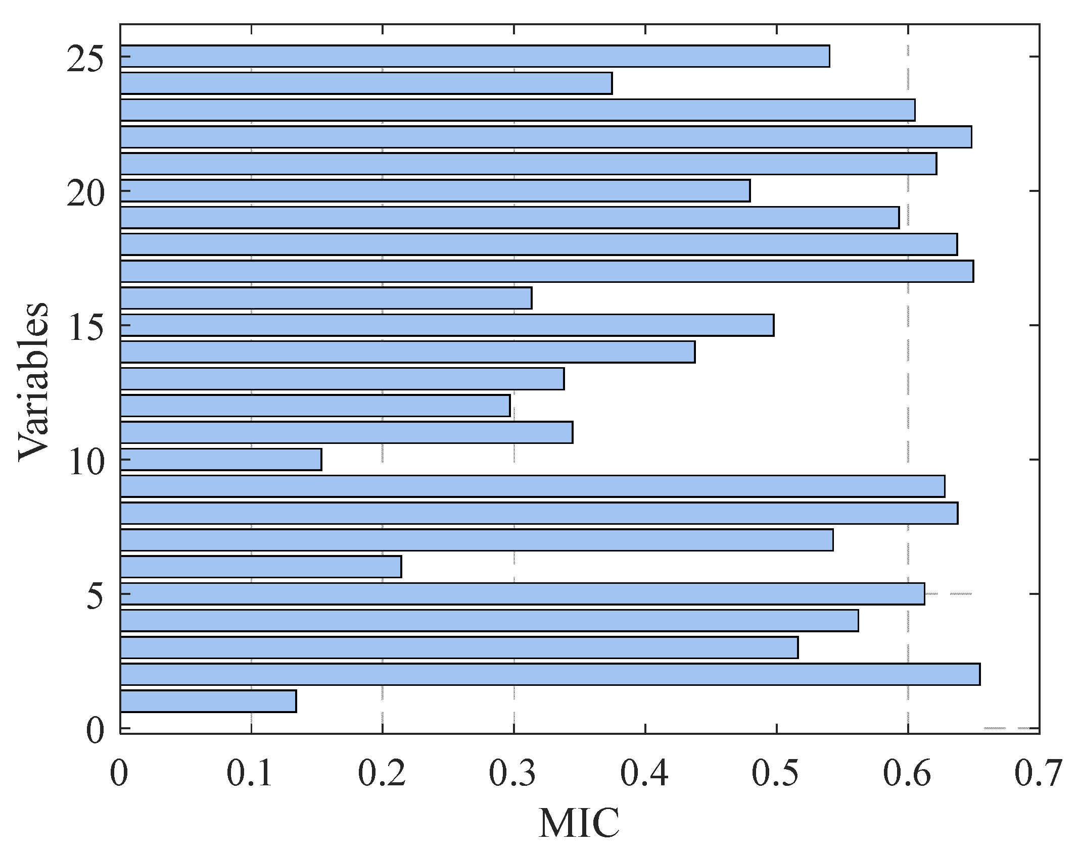
- We introduce a novel feature selection method based on the MIC. This approach effectively identifies key input variables and their optimal input order, significantly improving both the efficiency and accuracy of feature selection compared to traditional methods.
- A novel Trans-GRU network is proposed for multi-step forecasting. This network combines the strengths of Transformer models in capturing long-sequence dependencies with the capabilities of GRU models in modeling local temporal features. The Trans-GRU network enables the simultaneous capture of multivariate correlations and the learning of global sequence representations, addressing the limitations of GRU models in modeling long sequences and overcoming the weakness of Transformer models in industrial forecasting applications.
- The proposed approach significantly enhances the accuracy of multi-step methane content prediction. This improved predictive capability supports the stable operation and optimization of the steam reforming process in hydrogen production. Additionally, it provides a valuable reference for multi-step prediction of dynamic, non-stationary industrial data in various industrial processes.
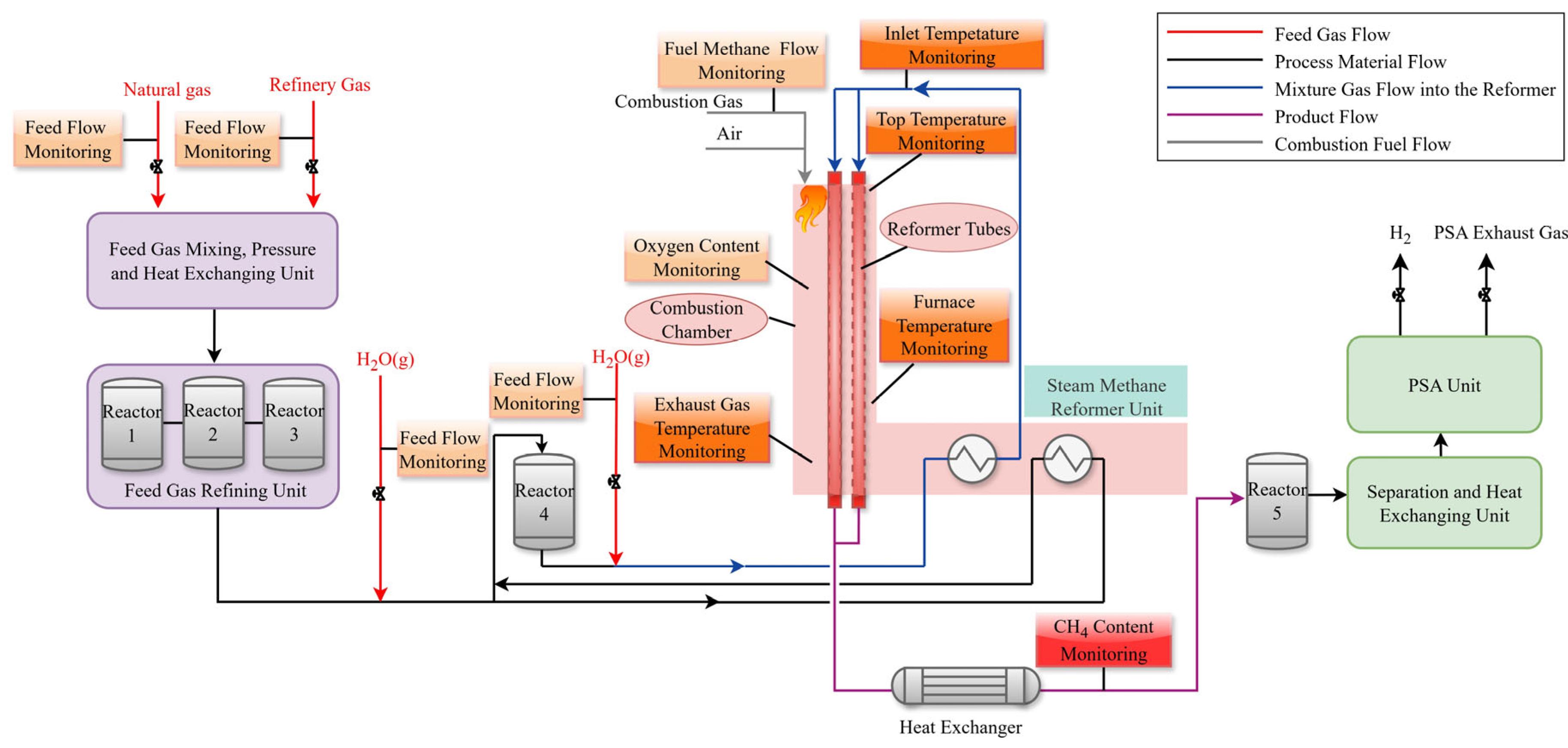
2. Process Description
3. Intelligent Model for Multi-Step Forecasting
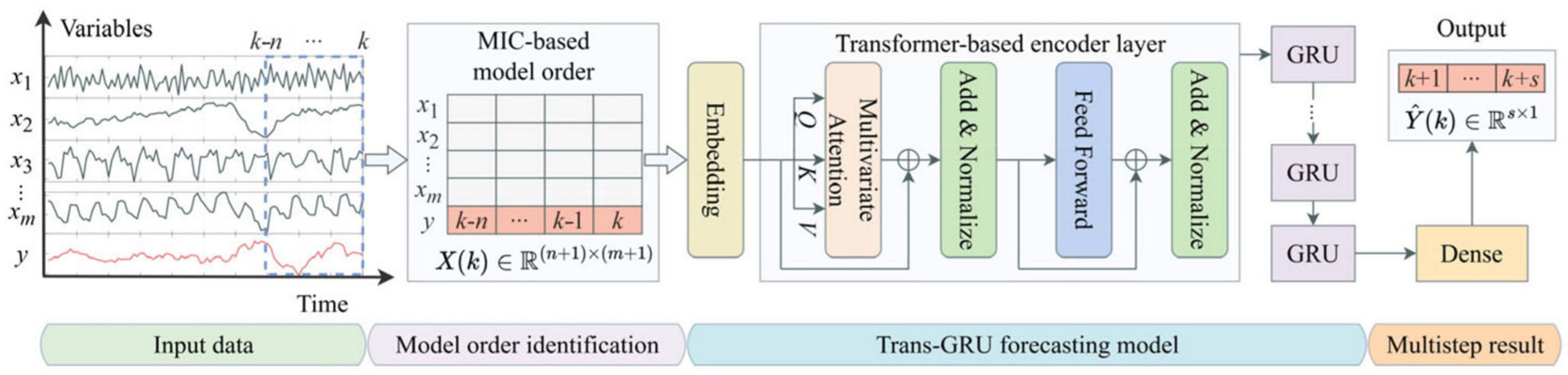
3.1. Structure Overview
3.2. Model Order Determination
3.3. Feature Extraction Based on Transformer-Encoding Modeling
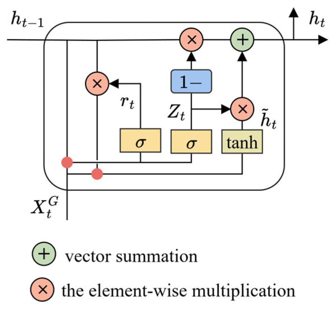
3.4. Multi-Step Forecasting Based on GRU Model
4. Results and Discussion
4.1. Data Description
4.2. Model Order Selection Mechanism
4.3. Implementation Details
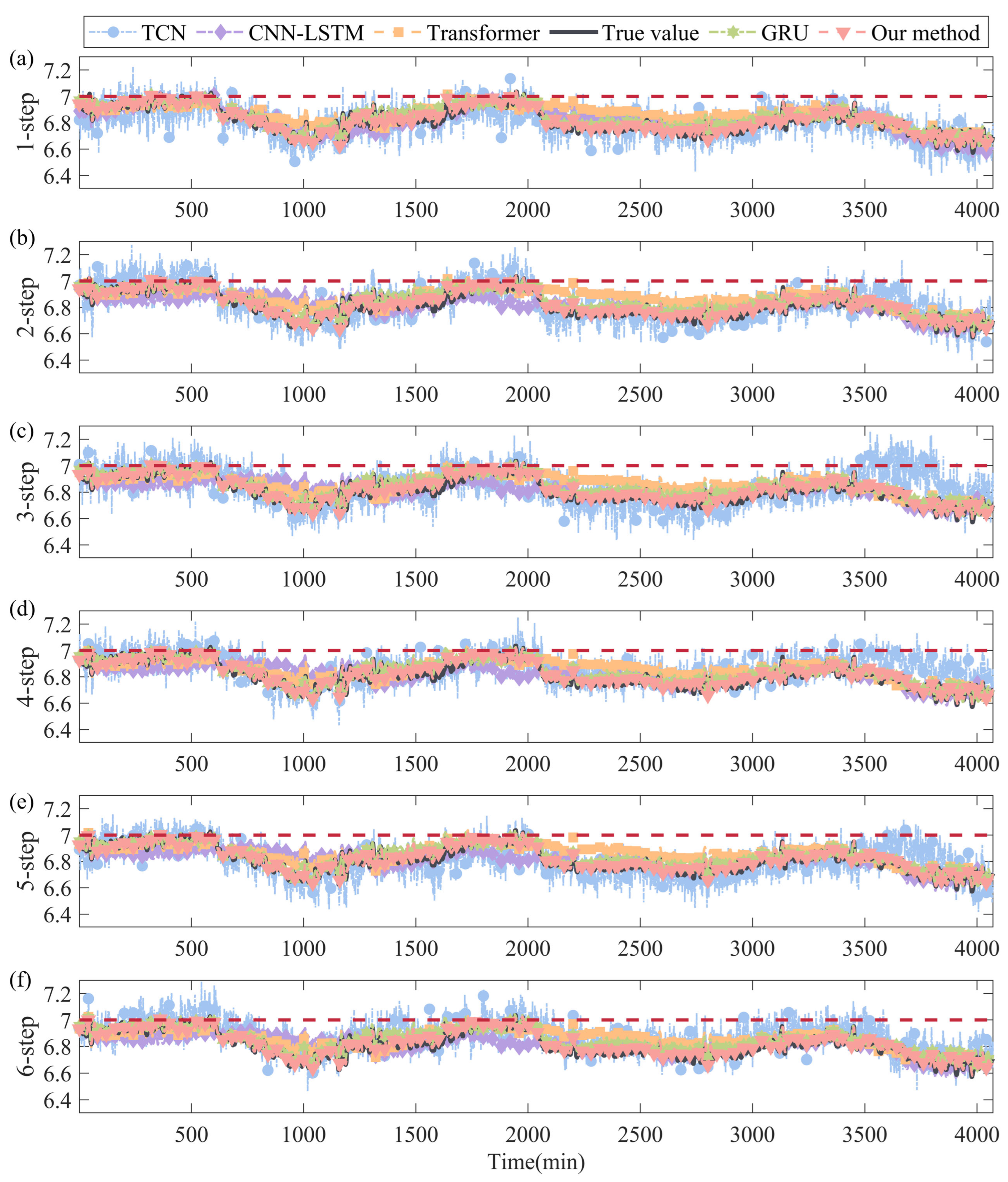
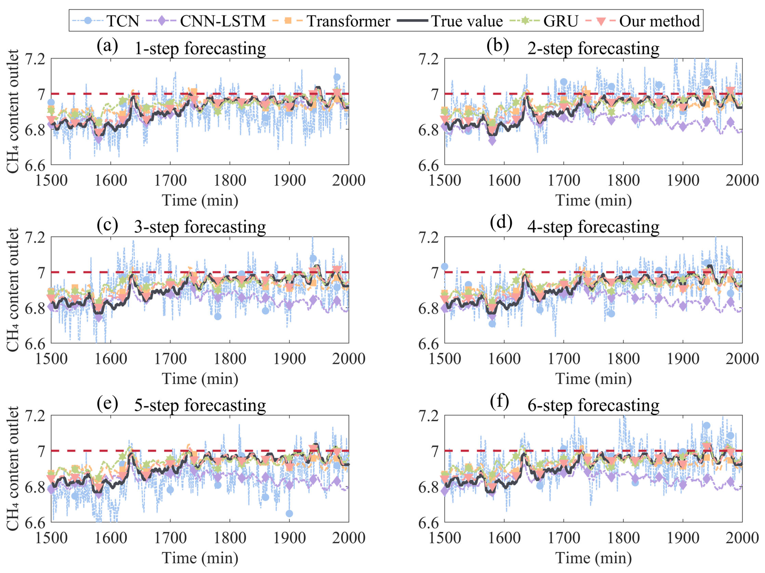
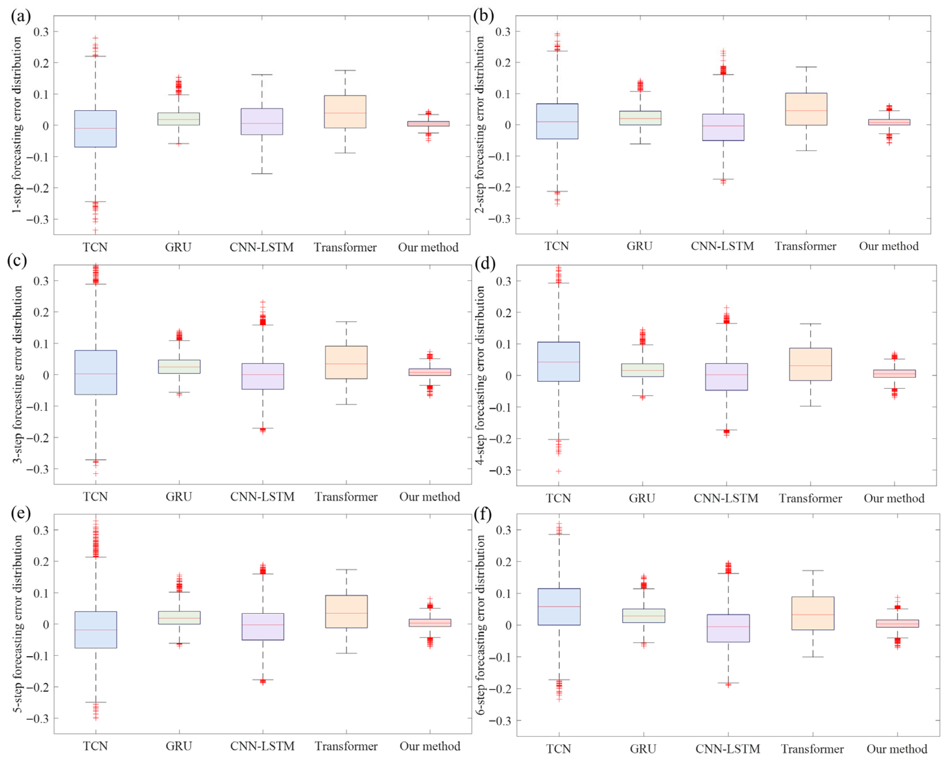
4.4. Multi-Step-Ahead Forecasting Results
5. Conclusions
Author Contributions
Funding
Data Availability Statement
Conflicts of Interest
References
- Midilli, A.; Ay, M.; Dincer, I.; Rosen, M.A. On hydrogen and hydrogen energy strategies: I: Current status and needs. Renew. Sustain. Energy Rev. 2005, 9, 255–271. [Google Scholar] [CrossRef]
- Winter, C.-J. Hydrogen energy—Abundant, efficient, clean: A debate over the energy-system-of-change. Int. J. Hydrogen Energy 2009, 34, S1–S52. [Google Scholar] [CrossRef]
- Gunathilake, C.; Soliman, I.; Panthi, D.; Tandler, P.; Fatani, O.; Ghulamullah, N.A.; Marasinghe, D.; Farhath, M.; Madhujith, T.; Conrad, K.; et al. A comprehensive review on hydrogen production, storage, and applications. Chem. Soc. Rev. 2024, 53, 10900–10969. [Google Scholar] [CrossRef] [PubMed]
- Chaubey, R.; Sahu, S.; James, O.O.; Maity, S.J.R.; Reviews, S.E. A review on development of industrial processes and emerging techniques for production of hydrogen from renewable and sustainable sources. Renew. Sustain. Energy Rev. 2013, 23, 443–462. [Google Scholar] [CrossRef]
- Amini, A.; Bagheri, A.A.H.; Sedaghat, M.H.; Rahimpour, M.R. CFD simulation of an industrial steam methane reformer: Effect of burner fuel distribution on hydrogen production. Fuel 2023, 352, 129008. [Google Scholar] [CrossRef]
- Xu, J.; Froment, G.F.J.A.J. Methane steam reforming, methanation and water-gas shift: I. Intrinsic kinetics. AIChE J. 1989, 35, 88–96. [Google Scholar] [CrossRef]
- Peng, X.; Jin, Q. Molecular simulation of methane steam reforming reaction for hydrogen production. Int. J. Hydrogen Energy 2022, 47, 7569–7585. [Google Scholar] [CrossRef]
- Proell, T.; Lyngfelt, A.J.E. Steam methane reforming with chemical-looping combustion: Scaling of fluidized-bed-heated reformer tubes. Energy Fuel 2022, 36, 9502–9512. [Google Scholar] [CrossRef]
- Amirshaghaghi, H.; Zamaniyan, A.; Ebrahimi, H.; Zarkesh, M.J.A.M.M. Numerical simulation of methane partial oxidation in the burner and combustion chamber of autothermal reformer. Appl. Math. Model. 2010, 34, 2312–2322. [Google Scholar] [CrossRef]
- Noh, Y.S.; Lee, K.-Y.; Moon, D.J. Hydrogen production by steam reforming of methane over nickel based structured catalysts supported on calcium aluminate modified SiC. Int. J. Hydrogen Energy 2019, 44, 21010–21019. [Google Scholar] [CrossRef]
- Ighalo, J.O.; Amama, P.B. Recent advances in the catalysis of steam reforming of methane (SRM). Int. J. Hydrogen Energy 2024, 51, 688–700. [Google Scholar] [CrossRef]
- Wang, M.; Tan, X.; Motuzas, J.; Li, J.; Liu, S.J.J.o.M.S. Hydrogen production by methane steam reforming using metallic nickel hollow fiber membranes. J. Membr. Sci. 2020, 620, 118909. [Google Scholar] [CrossRef]
- Kumar, A.; Baldea, M.; Edgar, T.F. A physics-based model for industrial steam-methane reformer optimization with non-uniform temperature field. Comput. Chem. Eng. 2017, 105, 224–236. [Google Scholar] [CrossRef]
- Olivieri, A.; Vegliò, F. Process simulation of natural gas steam reforming: Fuel distribution optimisation in the furnace. Fuel Process. Technol. 2008, 89, 622–632. [Google Scholar] [CrossRef]
- Lai, G.-H.; Lak, J.H.; Tsai, D.-H. Hydrogen production via low-temperature steam-methane reforming using Ni–CeO2–Al2O3 Hybrid Nanoparticle Clusters as Catalysts. ACS Appl. Energy Mater. 2019, 2, 7963–7971. [Google Scholar] [CrossRef]
- Rogers, J.L.; Mangarella, M.C.; D’Amico, A.D.; Gallagher, J.R.; Dutzer, M.R.; Stavitski, E.; Miller, J.T.; Sievers, C. Differences in the nature of active sites for methane dry reforming and methane steam reforming over nickel aluminate catalysts. ACS Catal. 2016, 6, 5873–5886. [Google Scholar] [CrossRef]
- Severson, K.; Chaiwatanodom, P.; Braatz, R.D. Perspectives on process monitoring of industrial systems. Annu. Rev. Control 2016, 42, 190–200. [Google Scholar] [CrossRef]
- Zhu, Z.; Lei, Y.; Qi, G.; Chai, Y.; Mazur, N.; An, Y.; Huang, X. A review of the application of deep learning in intelligent fault diagnosis of rotating machinery. Measurement 2023, 206, 112346. [Google Scholar] [CrossRef]
- Venkatasubramanian, V.; Rengaswamy, R.; Kavuri, S.N. A review of process fault detection and diagnosis: Part II: Qualitative models and search strategies. Comput. Chem. Eng. 2003, 27, 313–326. [Google Scholar] [CrossRef]
- Kumar, A.; Bhattacharya, A.; Flores-Cerrillo, J. Data-driven process monitoring and fault analysis of reformer units in hydrogen plants: Industrial application and perspectives. Comput. Chem. Eng. 2020, 136, 106756. [Google Scholar] [CrossRef]
- Kano, M.; Nakagawa, Y. Data-based process monitoring, process control, and quality improvement: Recent developments and applications in steel industry. Comput. Chem. Eng. 2008, 32, 12–24. [Google Scholar] [CrossRef]
- Lecun, Y.; Bengio, Y.; Hinton, G. Deep learning. Nature 2015, 521, 436. [Google Scholar] [CrossRef] [PubMed]
- Wang, Q.; Han, J.; Chen, F.; Zhang, X.; Yun, C.; Dou, Z.; Yan, T.; Yang, G. Real-time risk prediction of chemical processes based on attention-based Bi-LSTM. Chin. J. Chem. Eng. 2024, 75, 131–141. [Google Scholar] [CrossRef]
- Wang, Y.; Qian, C.; Qin, S.J. Attention-mechanism based DiPLS-LSTM and its application in industrial process time series big data prediction. Comput. Chem. Eng. 2023, 176, 108296. [Google Scholar] [CrossRef]
- Ding, C.; Yang, M.; Zhao, Y.; Du, W. Graph convolutional network for axial concentration profiles prediction in simulated moving bed. Chin. J. Chem. Eng. 2024, 73, 270–280. [Google Scholar] [CrossRef]
- Liu, D.; Wang, Y.; Liu, C.; Yuan, X.; Wang, K. KSLD-TNet: Key sample location and distillation transformer network for multistep ahead prediction in industrial processes. IEEE Sens. J. 2024, 24, 1792–1802. [Google Scholar] [CrossRef]
- Yuan, X.; Huang, L.; Ye, L.; Wang, Y.; Wang, K.; Yang, C.; Gui, W.; Shen, F. Quality prediction modeling for industrial processes using multiscale Attention-Based Convolutional Neural network. IEEE T. Cybern. 2024, 54, 2696–2707. [Google Scholar] [CrossRef] [PubMed]
- Li, Y.; Cao, H.; Li, Z.; Du, W.; Shen, W. A flexible multi-step prediction architecture for process variable monitoring in chemical intelligent manufacturing. Chem. Eng. Sci. 2025, 316, 121943. [Google Scholar] [CrossRef]
- Li, Y.; Cao, H.; Wang, X.; Yang, Z.; Li, N.; Shen, W. A new Correlation-Similarity Conjoint Algorithm for developing Encoder-Decoder based deep learning multi-step prediction model of chemical process. Chem. Eng. Sci. 2024, 288, 119748. [Google Scholar] [CrossRef]
- Liu, X.; Yang, L.; Zhang, Z. Short-term multi-step ahead wind power predictions based on a novel deep convolutional recurrent network method. IEEE Trans. Sustain. Energy 2021, 12, 1820–1833. [Google Scholar] [CrossRef]
- Zhou, Y.; Li, Y.; Liu, W. A multi-step ahead global solar radiation prediction method using an attention-based transformer model with an interpretable mechanism. Int. J. Hydrogen Energy 2023, 48, 15317–15330. [Google Scholar] [CrossRef]
- Dai, J.; Ling, P.; Shi, H.; Liu, H. A multi-step furnace temperature prediction model for regenerative aluminum smelting based on reversible instance Normalization-Convolutional Neural Network-Transformer. Processes 2024, 12, 2438. [Google Scholar] [CrossRef]
- Vaswani, A.; Shazeer, N.; Parmar, N.; Uszkoreit, J.; Jones, L.; Gomez, A.N.; Kaiser, L.; Polosukhin, I. Attention is all you need. In Proceedings of the 31st Annual Conference on Neural Information Processing Systems (NIPS), Long Beach, CA, USA, 4–9 December 2017. [Google Scholar]
- Xia, M.; Shao, H.; Ma, X.; De Silva, C. A stacked GRU-RNN-Based approach for predicting renewable energy and electricity load for smart grid operation. IEEE Trans. Ind. Inf. 2021, 17, 7050–7059. [Google Scholar] [CrossRef]
- Zeng, A.; Chen, M.-H.; Zhang, L.; Xu, Q. Are transformers effective for time series forecasting? In Proceedings of the AAAI Conference on Artificial Intelligence, Washington, DC, USA, 7–14 February 2023. [Google Scholar]
- Dey, R.; Salemt, F.M. Gate-variants of Gated Recurrent Unit (GRU) neural networks. In Proceedings of the IEEE International Midwest Symposium on Circuits & Systems, Boston, MA, USA, 6–9 August 2017. [Google Scholar]
- Yang, J.; Chai, T.Y.; Luo, C.M.; Yu, W. Intelligent demand forecasting of smelting process using data-driven and mechanism model. IEEE Trans. Ind. Electron. 2019, 66, 9745–9755. [Google Scholar] [CrossRef]
- Zhang, Y.; Jia, S.L.; Huang, H.Y.; Qiu, J.Q.; Zhou, C.J. A novel algorithm for the precise calculation of the maximal information coefficient. Sci. Rep. 2014, 4, 6662. [Google Scholar] [CrossRef] [PubMed]
- Lea, C.; Vidal, R.; Reiter, A.; Hager, G.D. Temporal convolutional networks: A unified approach to action segmentation. In Proceedings of the 14th European Conference on Computer Vision (ECCV), Amsterdam, The Netherlands, 8–16 October 2016. [Google Scholar]
- Chung, J.; Gulcehre, C.; Cho, K.H.; Bengio, Y.J.E.A. Empirical evaluation of gated recurrent neural networks on sequence modeling. arXiv, 2014; arXiv:1412.3555. [Google Scholar] [CrossRef]
- Kim, T.Y.; Cho, S.B. Predicting residential energy consumption using CNN-LSTM neural networks. Energy 2019, 182, 72–81. [Google Scholar] [CrossRef]


| Variables | Parameters | Unit |
|---|---|---|
| x1 | Refinery gas volume flow rate | Nm3/h |
| x2 | Natural gas volume flow rate | Nm3/h |
| x3 | Overheated steam mass flow rate before pre-reforming reactions | t/h |
| x4 | Overheated steam mass flow rate after pre-reforming reactions | t/h |
| x5 | Gas volume flow rate | Nm3/h |
| x6 | Oxygen content in the combustion chamber | % |
| x7–9 | 1–3rd furnace temperature | °C |
| x10 | Inlet temperature at reformer tubes | °C |
| x11–15 | 1–4th top temperature at reformer | °C |
| x16–25 | 1–10th temperature of flue gas discharged from reformer | °C |
| y | Methane content at heat exchanger outlet | % |
| Models | 1-Step | 2-Step | 3-Step | 4-Step | 5-Step | 6-Step | ||||||
|---|---|---|---|---|---|---|---|---|---|---|---|---|
| RMSE | MAE | RMSE | MAE | RMSE | MAE | RMSE | MAE | RMSE | MAE | RMSE | MAE | |
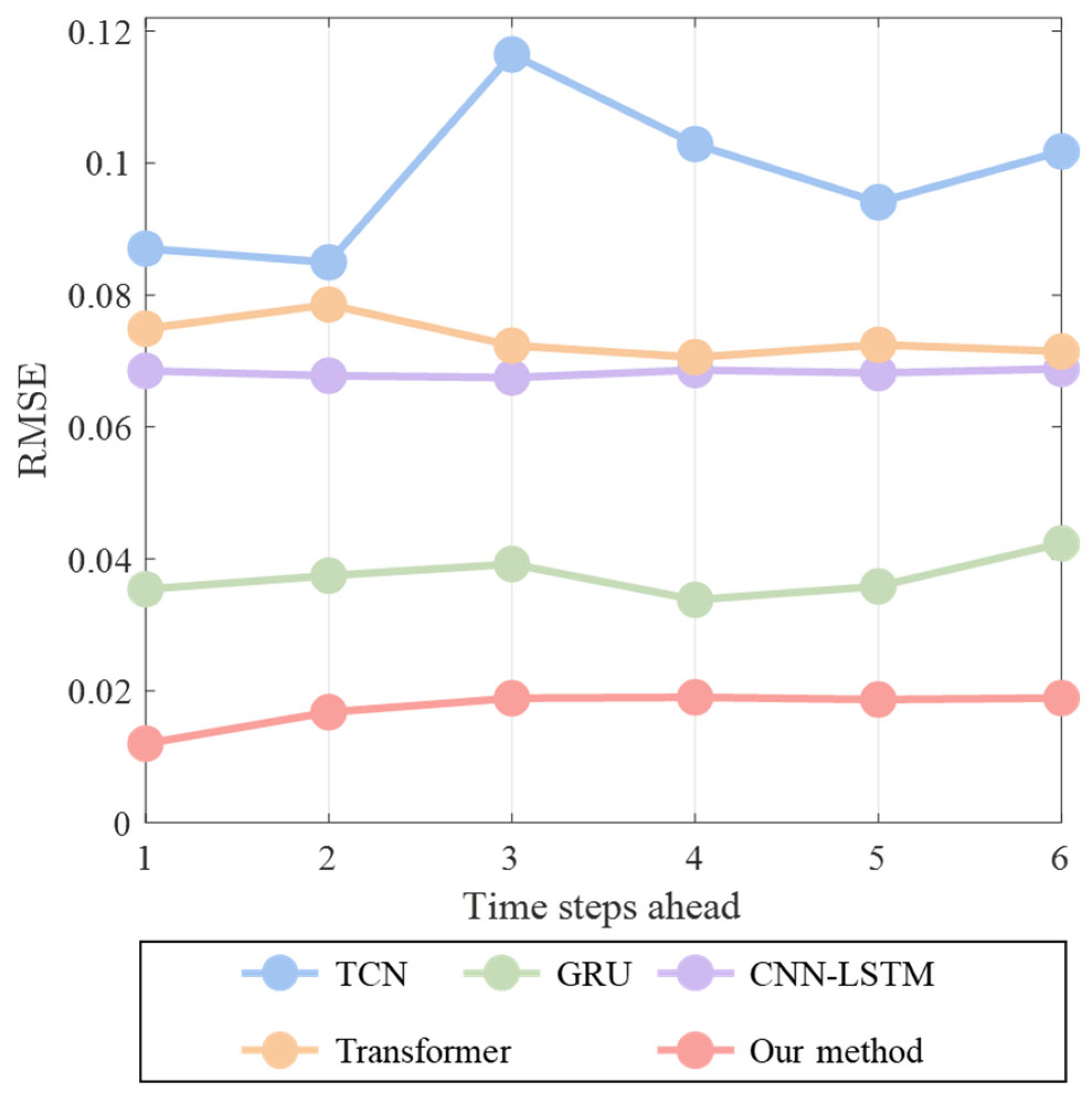
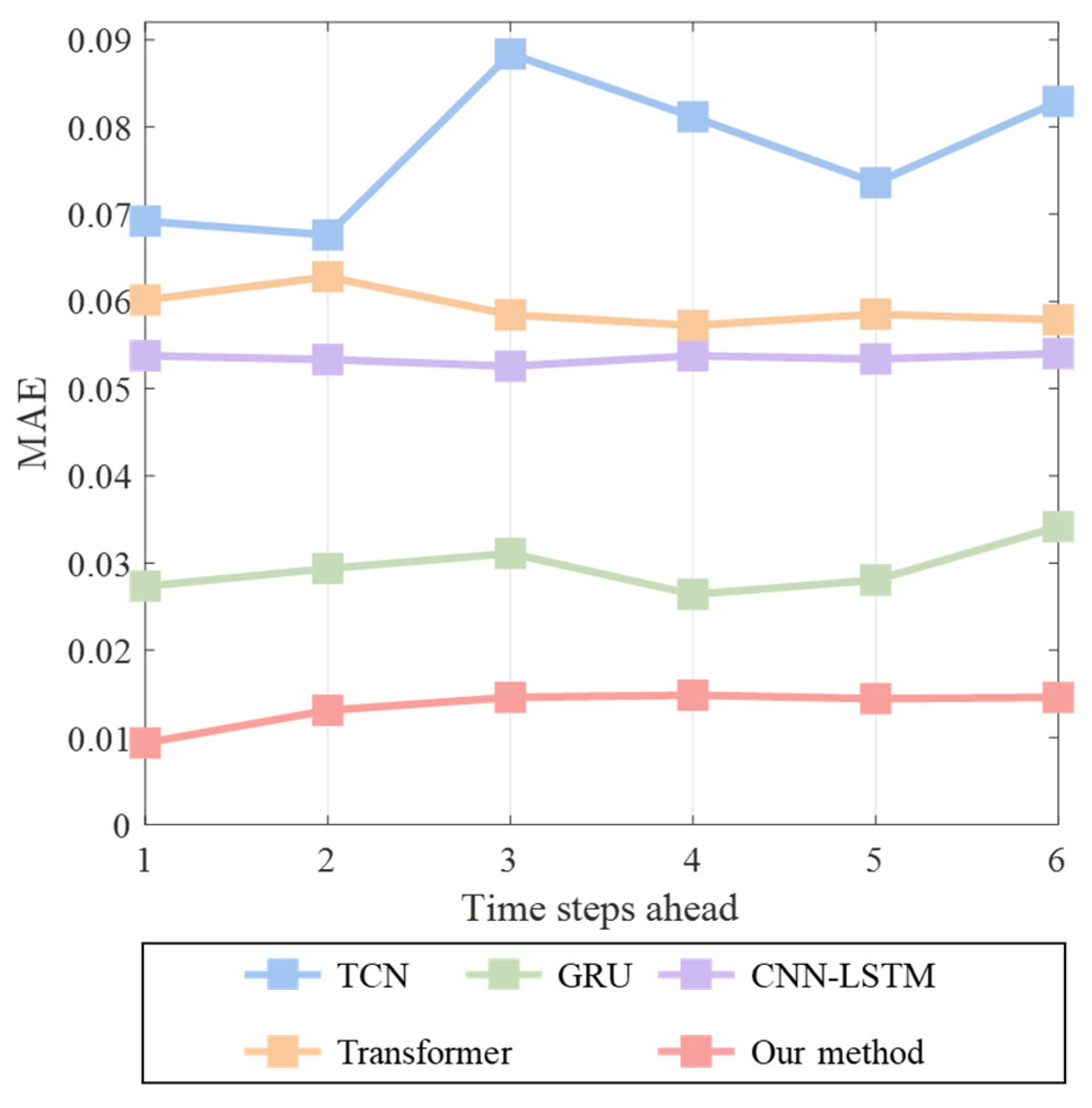
| TCN | 0.0870 | 0.0692 | 0.0849 | 0.0676 | 0.1165 | 0.0884 | 0.1029 | 0.0812 | 0.0941 | 0.0736 | 0.1018 | 0.0829 |
| GRU | 0.0354 | 0.0273 | 0.0374 | 0.0294 | 0.0392 | 0.0311 | 0.0338 | 0.0264 | 0.0358 | 0.0281 | 0.0424 | 0.0342 |
| CNN-LSTM | 0.0685 | 0.0538 | 0.0678 | 0.0533 | 0.0675 | 0.0526 | 0.0686 | 0.0538 | 0.0682 | 0.0534 | 0.0688 | 0.0540 |
| Transformer | 0.0749 | 0.0602 | 0.0785 | 0.0628 | 0.0723 | 0.0585 | 0.0706 | 0.0572 | 0.0724 | 0.0585 | 0.0714 | 0.0579 |
| Our method | 0.0120 | 0.0094 | 0.0168 | 0.0131 | 0.0189 | 0.0146 | 0.0190 | 0.0149 | 0.0187 | 0.0145 | 0.0189 | 0.0146 |
Disclaimer/Publisher’s Note: The statements, opinions and data contained in all publications are solely those of the individual author(s) and contributor(s) and not of MDPI and/or the editor(s). MDPI and/or the editor(s) disclaim responsibility for any injury to people or property resulting from any ideas, methods, instructions or products referred to in the content. |
© 2025 by the authors. Licensee MDPI, Basel, Switzerland. This article is an open access article distributed under the terms and conditions of the Creative Commons Attribution (CC BY) license (https://creativecommons.org/licenses/by/4.0/).
Share and Cite
Zhang, Q.; Han, X.; Zhang, J.; Qin, P. A Hybrid Multi-Step Forecasting Approach for Methane Steam Reforming Process Using a Trans-GRU Network. Processes 2025, 13, 2313. https://doi.org/10.3390/pr13072313
Zhang Q, Han X, Zhang J, Qin P. A Hybrid Multi-Step Forecasting Approach for Methane Steam Reforming Process Using a Trans-GRU Network. Processes. 2025; 13(7):2313. https://doi.org/10.3390/pr13072313
Chicago/Turabian StyleZhang, Qinwei, Xianyao Han, Jingwen Zhang, and Pan Qin. 2025. "A Hybrid Multi-Step Forecasting Approach for Methane Steam Reforming Process Using a Trans-GRU Network" Processes 13, no. 7: 2313. https://doi.org/10.3390/pr13072313
APA StyleZhang, Q., Han, X., Zhang, J., & Qin, P. (2025). A Hybrid Multi-Step Forecasting Approach for Methane Steam Reforming Process Using a Trans-GRU Network. Processes, 13(7), 2313. https://doi.org/10.3390/pr13072313