
The Operational Nitrogen Indicator (ONI): An Intelligent Index for the Wastewater Treatment Plant’s Optimization

 , ,
, ,  , and
, and 
Abstract
1. Introduction
2. Approach
2.1. Operational Nitrogen Indicator—ONI
2.1.1. Indicator Structure
- Nreal% —the percentage of the legal limit reached for total nitrogen in the effluent. Equation (1) shows how it can be calculated.This metric evaluates compliance with the effluent nitrogen limits established via environmental legislation. Values approaching 100% indicate proximity to legal thresholds and a heightened risk of regulatory violation. The weight in ONI is 35%.
- Tnitr%—the temporal trend of total nitrogen. Equation (2) shows how it can be calculated.Calculated as the slope of a linear regression over a moving time window (typically 30–60 min), this indicator reflects the temporal evolution of nitrogen concentration. Rising trends suggest accumulation and potential instability in the biological process. The weight in ONI is 15%.
- Enitr%—nitrogen removal. Equation (3) shows how it can be calculated.This sub-indicator quantifies the process’s effectiveness in removing nitrogen from influent. High values (>75–80%) denote efficient operation; values below 60% typically indicate process underperformance or failure. The weight in ONI is 30%.
- NP%—nitrogen-to-phosphorus ratio as a microbial balance indicator. Equation (4) shows how it can be calculated.The N/P ratio is used to assess the stoichiometric balance necessary for optimal microbial growth. Ideal values typically range between 10 and 16, in line with established biological nutrient removal guidelines. Deviations from this range may indicate stress conditions or nutrient imbalance. The weight in ONI is 20%.
2.1.2. Interpretation Ranges
- ONI = 0–30 → optimal state: stable operation, no intervention required.
- ONI = 31–70 → attention status: Early deviations or suboptimal conditions are detected. Preventive operational adjustments are recommended.
- ONI > 70 → critical status: Imminent risk of failure or legal noncompliance. Requires immediate or automated intervention.
2.1.3. Technical–Operational and Regulatory Justification
Nreal%—Regulatory Compliance
Tnitr%—Dynamic Process Stability
Enitr%—Removal Efficiency
NP%—Microbiological Balance
Weighting Criteria
2.1.4. Summary of the ONI’s Objectives
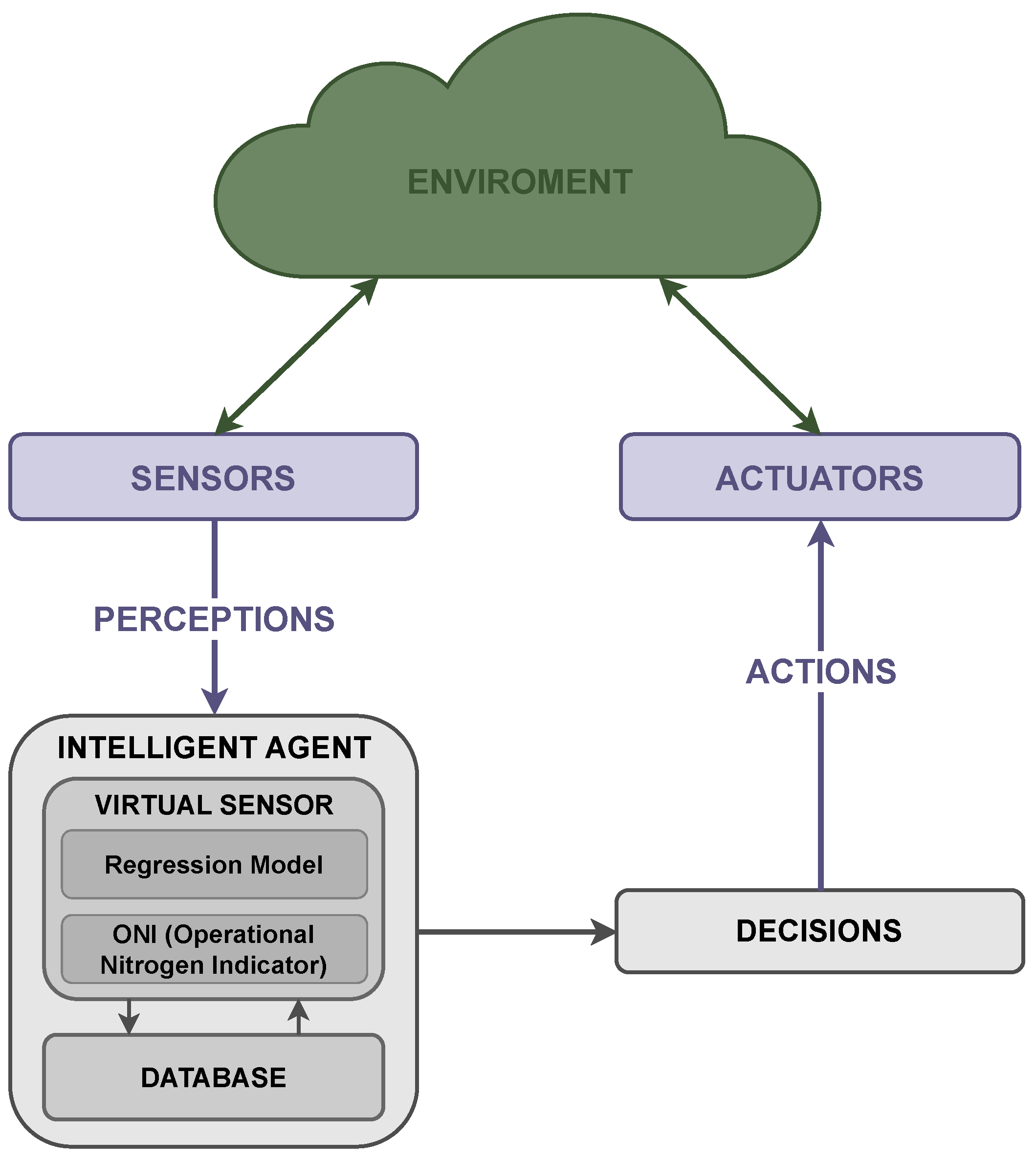
2.2. Agent-Based System Approach
2.2.1. Enviroment Description
2.2.2. Perception
2.2.3. Decision-Making
2.2.4. Action
2.2.5. System Integration
2.3. Intelligent Agent Architecture
2.3.1. Data Preprocessing
2.3.2. Virtual Sensor
2.3.3. Database
3. Case of Study
3.1. WWTP Description
3.2. Obtaining the Data Set
3.2.1. Data Set for Developing the Model
3.2.2. Data Set for Validating Agent Approach
4. Agent Model Implementation
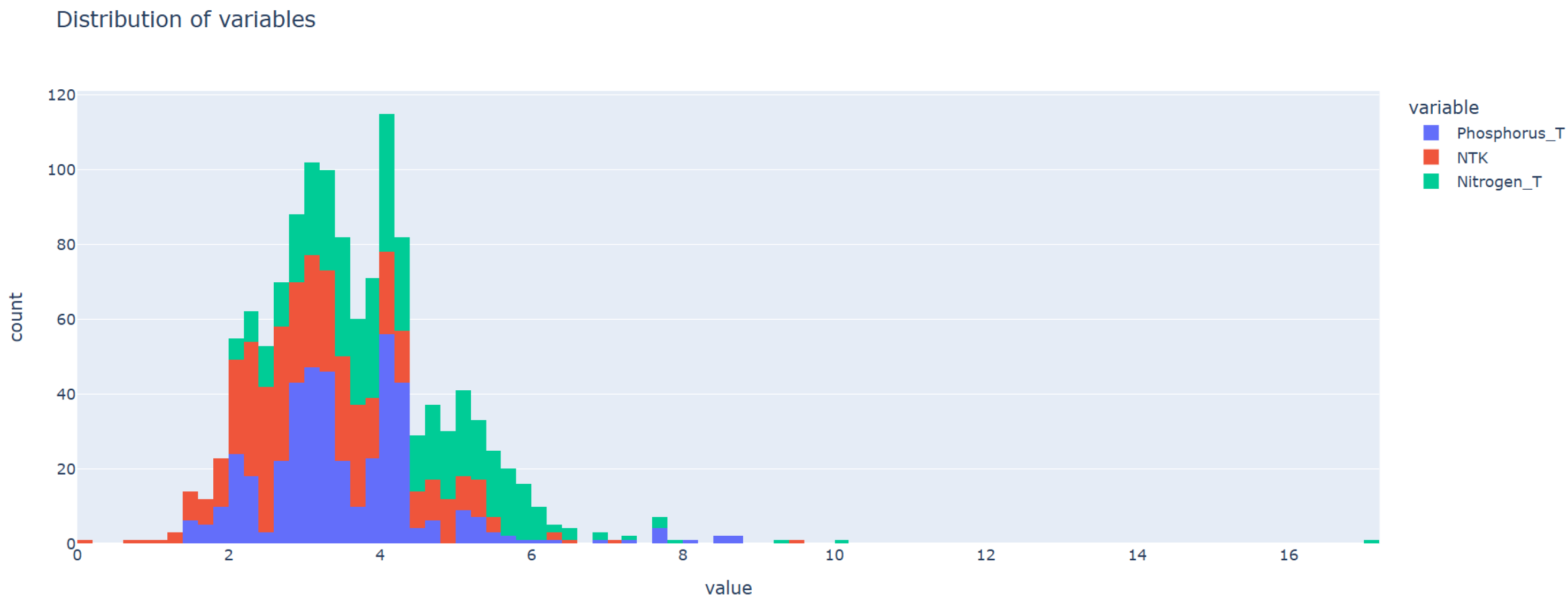
4.1. Data Set Preprocessing
4.2. Applied Methods
- Linear regression.
- Polynomial regression.
- K-nearest neighbors.
- Decision tree.
- Random forest.
- Gradient boosting.
- Support vector machine.
- Multi-layer perceptron.
4.2.1. Linear Regression
- Intercept: a boolean value that calculates the independent term (true) or sets it to zero (false).
- Positive: a boolean value that forces the coefficients to be positive (true) or to take any value (false).
4.2.2. Polynomial Regression
- Degree: an integer value that determines the degree of the polynomial, that is, the highest power of any variable.
- include_bias: a boolean value that calculates the independent term (true) or sets it to zero (false).
- interaction_only: a boolean value that sets whether to include only interaction terms without powers (true).
4.2.3. K-Nearest Neighbors
- n_neighbors: a natural value that determines the number K of neighbors used for the prediction.
- Weights: A function that assigns the importance (weight) of each of the K neighbors in the prediction.
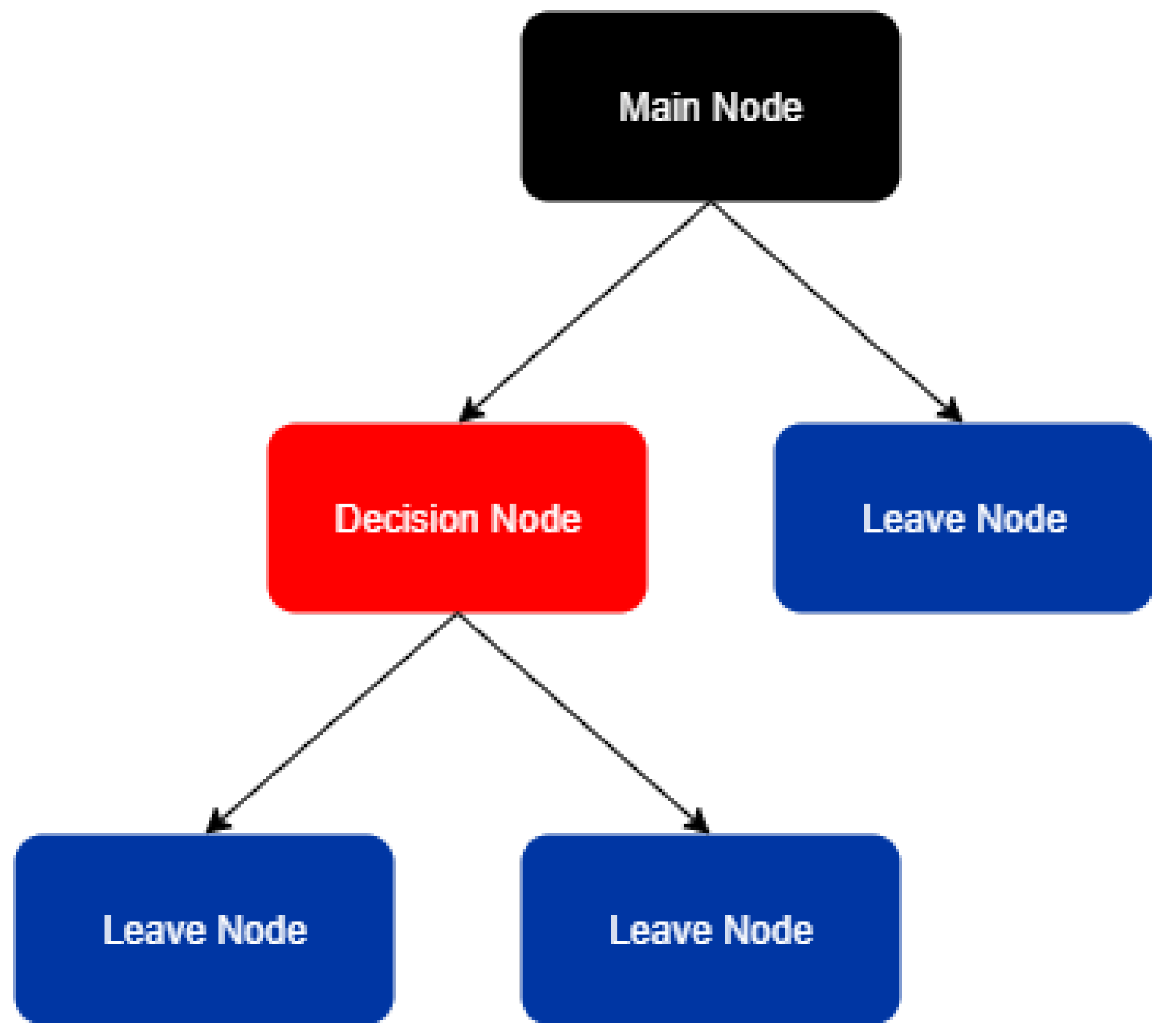
4.2.4. Decision Tree
- max_depth: a natural value that determines the maximum depth of the diagram.
- criterion: the function used to determine the quality of the division performed during the training process.
- splitter: the strategy used to select the division at each node during the training process.
4.2.5. Random Forest
- n_estimators: a natural value that determines the number of decision trees used.
- max_depth: a natural value that determines the maximum depth of the diagram.
- criterion: the function used to determine the quality of the division performed during the training process.
4.2.6. Gradient Boosting
- Loss: the cost function to be minimized.
- learning_rate: a floating point number that determines the model’s learning rate. It controls the contribution of each decision tree.
- n_estimators: a natural value that determines the number of decision trees used.
- Criterion: the function used to determine the quality of the division performed during the training process.
4.2.7. Support Vector Machine
- Kernel:
- C: or regularization coefficient, a floating-point number that controls the penalty.
- Epsilon: a floating-point number that determines the tolerance margin.
4.2.8. Multi-Layer Perceptron
- hidden_neurons: a natural number that determines the number of neurons in the hidden layer.
- Dropout: a floating point number that determines the proportion of neurons that are canceled.
- activation_function: a function that determines the neuron’s output based on its inputs.
4.3. Experiment Setup
4.3.1. Data Set
4.3.2. Regression Model Implementation
Linear Regression
- Calculation and assignment of 0 for the independent term.
- Force the coefficients to be positive and allow them to take any value.
Polynomial Regression
- Calculation and assignment to 0 of the independent term.
- Degree of the polynomial between 2 and 7.
K-Nearest Neighbors
- Values of n_neighbours from 1 to 99, taking all odd numbers.
- Uniform and distance-based weight assignment.
Decision Tree
- All odd values from 1 to 59 were taken for the depth of the diagram.
- The Poisson, absolute error, and mean squared error functions with Friedman’s improvement to calculate splitting quality.
- The selection of the division according to the best option and randomly.
Random Forest
- From 1 to 59 regressors, always odd numbers, were used to create the forest.
Gradient Boosting
- The squared error, the absolute error, and the Huber function were used as the loss function.
- The following values were used as learning rates: 0.001, 0.005, 0.01, 0.05, 0.1, 0.5, 1, 5, and 10.
- Values from 10 to 200, in increments of 10, were used for the number of boosting stages to perform.
- The squared error and mean squared error functions with Friedman’s improvement for calculating splitting quality.
Support Vector Machine
- The radial basis function (RBF), sigmoidal function, and linear function were used as kernels.
- The following values were used as regularization coefficient values: 0.001, 0.005, 0.01, 0.05, 0.1, 0.5, 1, 5, 10, 50, and 100.
- The values 0.001, 0.005, 0.01, 0.05, 0.1, 0.5, 1, 5, and 10 were used in the epsilon hyperparameter ().
Multi-Layer Perceptron
- 1 to 50 neurons were used in the hidden layer.
- As dropout values, 0.1, 0.2, and 0.3 were used.
- The activation functions tested were ReLU, the hyperbolic tangent (tanh), sigmoid, and linear.
4.3.3. Regression Model Validation
Mean Absolute Error
- n is the total number of samples.
- yi is the actual ith value.
- is the predicted ith value.
Mean Square Error
- n is the total number of samples.
- yi is the actual ith value.
- is the predicted ith value.
Symmetric Mean Absolute Percentage Error
- n is the total number of samples.
- yi is the actual ith value.
- is the predicted ith value.
Coefficient of Determination
- n is the total number of samples.
- yi is the actual ith value.
- is the predicted ith value.
- is the mean value of the actual values.
4.4. Results
4.4.1. Regression Model Implementation
Linear Regression
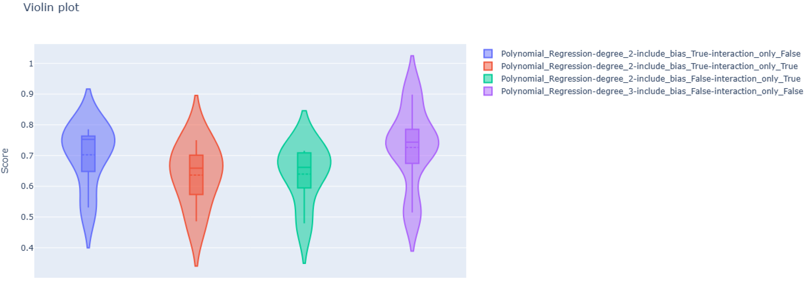
Polynomial Regression
K-Nearest Neighbors
Decision Tree
Random Forest
Gradient Boosting
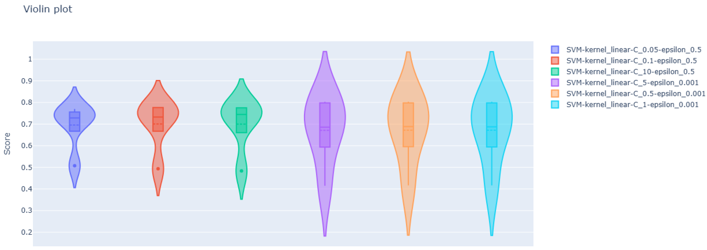
Support Vector Machine
Multi-Layer Perceptron
4.4.2. Regression Model Validation
4.4.3. Virtual Sensor Validation
5. Conclusions and Future Works
Author Contributions
Funding
Data Availability Statement
Conflicts of Interest
Abbreviations
| DT | Decision Tree |
| GB | Gradient Boosting |
| KNNs | K-Nearest Neighbors |
| LR | Linear Regression |
| MAE | Mean Absolute Error |
| MLP | Multi-Layer Perceptron |
| MSE | Mean Squared Error |
| ONI | Operational Nitrogen Indicator |
| PR | Polynomial Regression |
| R2 | Coefficient of Determination |
| RBF | Radial Basis Function |
| ReLU | Rectified Linear Unit |
| RF | Random Forest |
| SMAPE | Symmetric Mean Absolute Percentage Error |
| SVM | Support Vector Machine |
| tanh | Hyperbolic tangent |
| TKN | Total Kjeldahl Nitrogen |
| WWTP | Waste Water Treatment Plant |
References
- Şenol, R.; Salman, O.; Kaya, Z. Potable water production from ambient moisture. Appl. Water Sci. 2023, 13, 10. [Google Scholar] [CrossRef]
- Brown, T.C.; Mahat, V.; Ramirez, J.A. Adaptation to future water shortages in the United States caused by population growth and climate change. Earth’s Future 2019, 7, 219–234. [Google Scholar] [CrossRef]
- Boretti, A.; Rosa, L. Reassessing the projections of the world water development report. NPJ Clean Water 2019, 2, 15. [Google Scholar] [CrossRef]
- Safarpour, H.; Tabesh, M.; Shahangian, S.A. Environmental Assessment of a Wastewater System under Water demand management policies. Water Resour. Manag. 2022, 36, 2061–2077. [Google Scholar] [CrossRef]
- Spellman, F.R. Handbook of Water and Wastewater Treatment Plant Operations; CRC Press: Boca Raton, FL, USA, 2013. [Google Scholar]
- Ianes, J.; Cantoni, B.; Remigi, E.U.; Polesel, F.; Vezzaro, L.; Antonelli, M. A stochastic approach for assessing the chronic environmental risk generated by wet-weather events from integrated urban wastewater systems. Environ. Sci. Water Res. Technol. 2023, 9, 3174–3190. [Google Scholar] [CrossRef]
- Mascher, F.; Mascher, W.; Pichler-Semmelrock, F.; Reinthaler, F.F.; Zarfel, G.E.; Kittinger, C. Impact of Combined Sewer Overflow on Wastewater Treatment and Microbiological Quality of Rivers for Recreation. Water 2017, 9, 906. [Google Scholar] [CrossRef]
- Lu, J.Y.; Wang, X.M.; Liu, H.Q.; Yu, H.Q.; Li, W.W. Optimizing operation of municipal wastewater treatment plants in China: The remaining barriers and future implications. Environ. Int. 2019, 129, 273–278. [Google Scholar] [CrossRef] [PubMed]
- Bertanza, G.; Boiocchi, R.; Pedrazzani, R. Improving the quality of wastewater treatment plant monitoring by adopting proper sampling strategies and data processing criteria. Sci. Total Environ. 2022, 806, 150724. [Google Scholar] [CrossRef] [PubMed]
- Kizgin, A.; Schmidt, D.; Joss, A.; Hollender, J.; Morgenroth, E.; Kienle, C.; Langer, M. Application of biological early warning systems in wastewater treatment plants: Introducing a promising approach to monitor changing wastewater composition. J. Environ. Manag. 2023, 347, 119001. [Google Scholar] [CrossRef] [PubMed]
- Longo, S.; d’Antoni, B.M.; Bongards, M.; Chaparro, A.; Cronrath, A.; Fatone, F.; Lema, J.M.; Mauricio-Iglesias, M.; Soares, A.; Hospido, A. Monitoring and diagnosis of energy consumption in wastewater treatment plants. A state of the art and proposals for improvement. Appl. Energy 2016, 179, 1251–1268. [Google Scholar] [CrossRef]
- Martínez, R.; Vela, N.; el Aatik, A.; Murray, E.; Roche, P.; Navarro, J.M. On the Use of an IoT Integrated System for Water Quality Monitoring and Management in Wastewater Treatment Plants. Water 2020, 12, 1096. [Google Scholar] [CrossRef]
- Thomas, O.; Théraulaz, F.; Cerdà, V.; Constant, D.; Quevauviller, P. Wastewater quality monitoring. TrAC Trends Anal. Chem. 1997, 16, 419–424. [Google Scholar] [CrossRef]
- Pehlivanoglu-Mantas, E.; Sedlak, D.L. Wastewater-Derived Dissolved Organic Nitrogen: Analytical Methods, Characterization, and Effects—A Review. Crit. Rev. Environ. Sci. Technol. 2006, 36, 261–285. [Google Scholar] [CrossRef]
- Bagherzadeh, F.; Mehrani, M.J.; Basirifard, M.; Roostaei, J. Comparative study on total nitrogen prediction in wastewater treatment plant and effect of various feature selection methods on machine learning algorithms performance. J. Water Process Eng. 2021, 41, 102033. [Google Scholar] [CrossRef]
- Ye, G.; Wan, J.; Deng, Z.; Wang, Y.; Chen, J.; Zhu, B.; Ji, S. Prediction of effluent total nitrogen and energy consumption in wastewater treatment plants: Bayesian optimization machine learning methods. Bioresour. Technol. 2024, 395, 130361. [Google Scholar] [CrossRef] [PubMed]
- Manami, M.; Seddighi, S.; Örlü, R. Deep learning models for improved accuracy of a multiphase flowmeter. Measurement 2023, 206, 112254. [Google Scholar] [CrossRef]
- Farsi, M.; Shojaei Barjouei, H.; Wood, D.A.; Ghorbani, H.; Mohamadian, N.; Davoodi, S.; Reza Nasriani, H.; Ahmadi Alvar, M. Prediction of oil flow rate through orifice flow meters: Optimized machine-learning techniques. Measurement 2021, 174, 108943. [Google Scholar] [CrossRef]
- Baggiani, F.; Marsili-Libelli, S. Real-time fault detection and isolation in biological wastewater treatment plants. Water Sci. Technol. 2009, 60, 2949–2961. [Google Scholar] [CrossRef] [PubMed]
- Sen, S.; Husom, E.J.; Goknil, A.; Politaki, D.; Tverdal, S.; Nguyen, P.; Jourdan, N. Virtual sensors for erroneous data repair in manufacturing a machine learning pipeline. Comput. Ind. 2023, 149, 103917. [Google Scholar] [CrossRef]
- Ko, D.; Norton, J.W., Jr.; Daigger, G.T. Wastewater management decision-making: A literature review and synthesis. Water Environ. Res. 2024, 96, e11024. [Google Scholar] [CrossRef] [PubMed]
- Holloway, T.G.; Williams, J.B.; Ouelhadj, D.; Cleasby, B. Process stress in municipal wastewater treatment processes: A new model for monitoring resilience. Process Saf. Environ. Prot. 2019, 132, 169–181. [Google Scholar] [CrossRef]
- Lai, J. Research on prediction algorithm of effluent quality and development of integrated control system for waste-water treatment. Sci. Rep. 2025, 15, 1–21. [Google Scholar] [CrossRef] [PubMed]
- Sharma, T.; Kumar, A.; Pant, S.; Kotecha, K. Wastewater Treatment and Multi-Criteria Decision-Making Methods: A Review. IEEE Access 2023, 11, 143704–143720. [Google Scholar] [CrossRef]
- Goulart Coelho, L.M.; Lange, L.C.; Coelho, H.M. Multi-criteria decision making to support waste management: A critical review of current practices and methods. Waste Manag. Res. 2017, 35, 3–28. [Google Scholar] [CrossRef] [PubMed]
- Wang, Y.; Cheng, Y.; Liu, H.; Guo, Q.; Dai, C.; Zhao, M.; Liu, D. A review on applications of artificial intelligence in wastewater treatment. Sustainability 2023, 15, 13557. [Google Scholar] [CrossRef]
- Council Directive 91/271/EEC of 21 May 1991 concerning urban waste-water treatment. Off. J. Eur. Communities 1991, L135, 40–52. Available online: https://eur-lex.europa.eu/legal-content/EN/TXT/?uri=CELEX:31991L0271 (accessed on 6 May 2025).
- Real Decreto 509/1996, de 15 de Marzo, por el que se Desarrolla el Real Decreto-Ley 11/1995, de 28 de Diciembre, Sobre Tratamiento de Aguas Residuales Urbanas. Boletín Oficial del Estado, n.º 77, 29 de Marzo de 1996, pp. 11290–11301. 1996. Available online: https://www.boe.es/eli/es/rd/1996/03/15/509 (accessed on 6 May 2025).
- Henze, M.; van Loosdrecht, M.C.; Ekama, G.A.; Brdjanovic, D. Biological Wastewater Treatment: Principles, Modelling and Design; IWA Publishing: London, UK, 2008. [Google Scholar]
- Oakley, S. Preliminary treatment and primary sedimentation. In Global Water Pathogen Project; California State University, Chico: Chico, CA, USA, 2021. [Google Scholar]
- Balku, S. Comparison between alternating aerobic–anoxic and conventional activated sludge systems. Water Res. 2007, 41, 2220–2228. [Google Scholar] [CrossRef] [PubMed]
- Patziger, M.; Kainz, H.; Hunze, M.; Józsa, J. Influence of secondary settling tank performance on suspended solids mass balance in activated sludge systems. Water Res. 2012, 46, 2415–2424. [Google Scholar] [CrossRef] [PubMed]
- Matamoros, V.; Salvadó, V. Evaluation of a coagulation/flocculation-lamellar clarifier and filtration-UV-chlorination reactor for removing emerging contaminants at full-scale wastewater treatment plants in Spain. J. Environ. Manag. 2013, 117, 96–102. [Google Scholar] [CrossRef] [PubMed]
- Orhon, D. Evolution of the activated sludge process: The first 50 years. J. Chem. Technol. Biotechnol. 2014, 90, 608–640. [Google Scholar] [CrossRef]
- Zagklis, D.P.; Bampos, G. Tertiary Wastewater Treatment Technologies: A Review of Technical, Economic, and Life Cycle Aspects. Processes 2022, 10, 2304. [Google Scholar] [CrossRef]
- Ayhan Demirbas, G.E.; Alalayah, W.M. Sludge production from municipal wastewater treatment in sewage treatment plant. Energy Sources Part A Recover. Util. Environ. Eff. 2017, 39, 999–1006. [Google Scholar] [CrossRef]
- Christensen, M.L.; Keiding, K.; Nielsen, P.H.; Jørgensen, M.K. Dewatering in biological wastewater treatment: A review. Water Res. 2015, 82, 14–24. [Google Scholar] [CrossRef] [PubMed]
- Athey, S.; Tibshirani, J.; Wager, S. Generalized random forests. Ann. Stat. 2019, 47, 1148–1178. [Google Scholar] [CrossRef]
- Popescu, M.C.; Balas, V.; Perescu-Popescu, L.; Mastorakis, N. Multilayer perceptron and neural networks. WSEAS Trans. Circuits Syst. 2009, 8, 579–588. [Google Scholar]


| Sub-Indicator | Meaning | Reference | Weight |
|---|---|---|---|
| Nreal% | N total vs. legal limit | 91/271/EEC [27]; RD 509/1996 [28] | 35% |
| Tnitr% | N trend () | Dynamic risk proxy; RD 509/1996 [28] | 15% |
| Enitr% | N removal efficiency | [27]; RD 509/1996 [28] | 30% |
| NP% | N/P balance | Redfield; Henze et al. [29] | 20% |
| ONI = | |||
| Input | Tag | Unit |
|---|---|---|
| Total Phosphorus | Phosp_T | mg/L |
| Total Kjeldahl Nitrogen | TKN | mg/L |
| Output | Tag | Unit |
| Total Nitrogen | Nitrogen_T | mg/L |
| Variable | Tag | Unit |
|---|---|---|
| Total Nitrogen at the Influent | Nitrogen_T_Influ | mg/L |
| Total Phosphorus | Phosp_T | mg/L |
| Total Kjeldahl Nitrogen | TKN | mg/L |
| Total Nitrogen | Nitrogen_T | mg/L |
| Metrics | ||||
|---|---|---|---|---|
| Configuration | R2 | MAE (mg/L) | MSE ((mg/L)2) | SMAPE (%) |
| intercept = True positive = True | 0.69319 | 0.45383 | 0.52564 | 5.36976 |
| intercept = True positive = False | 0.69319 | 0.45383 | 0.52564 | 5.36976 |
| intercept = False positive = True | 0.69691 | 0.45656 | 0.48700 | 5.46750 |
| intercept = False positive = False | 0.69691 | 0.45656 | 0.48700 | 5.46750 |
| Metrics | ||||
|---|---|---|---|---|
| Configuration | R2 | MAE (mg/L) | MSE ((mg/L)2) | SMAPE (%) |
| degree = 2 include_bias = True interaction_only = False | 0.64424 | 0.44368 | 0.58227 | 5.15816 |
| degree = 2 include_bias = True interaction_only = True | 0.63789 | 0.47783 | 0.64745 | 5.58262 |
| degree = 2 include_bias = False interaction_only = True | 0.62430 | 0.49164 | 0.65091 | 5.84100 |
| degree = 3 include_bias = False interaction_only = False | 0.62215 | 0.43200 | 0.57617 | 5.03020 |
| Metrics | ||||
|---|---|---|---|---|
| Configuration | R2 | MAE (mg/L) | MSE ((mg/L)2) | SMAPE (%) |
| K = 19 Weight = Uniform | 0.66872 | 0.43268 | 0.70421 | 5.00806 |
| K = 17 Weight = Uniform | 0.66805 | 0.42842 | 0.69923 | 4.94919 |
| K = 13 Weight = Uniform | 0.66792 | 0.42581 | 0.69037 | 4.90991 |
| K = 9 Weight = Distance | 0.64677 | 0.41969 | 0.68203 | 4.83718 |
| K = 11 Weight = Distance | 0.65179 | 0.41802 | 0.67720 | 4.81392 |
| K = 13 Weight = Distance | 0.65542 | 0.41787 | 0.67990 | 4.81108 |
| K = 15 Weight = Distance | 0.65354 | 0.41986 | 0.68707 | 4.83675 |
| Metrics | ||||
|---|---|---|---|---|
| Configuration | R2 | MAE (mg/L) | MSE ((mg/L)2) | SMAPE (%) |
| max_depth = 5 criterion = poisson splitter = best | 0.60805 | 0.45069 | 0.65623 | 5.26242 |
| max_depth = 5 criterion = absolute splitter = random | 0.57724 | 0.51034 | 0.88855 | 5.94258 |
| max_depth = 19 criterion = poisson splitter = random | 0.54750 | 0.50819 | 0.75363 | 6.17061 |
| max_depth = 5 criterion = friedman splitter = best | 0.52797 | 0.46268 | 0.75902 | 5.37417 |
| max_depth = 5 criterion = absolute splitter = best | 0.52692 | 0.45604 | 0.74765 | 5.19172 |
| max_depth = 7 criterion = poisson splitter = best | 0.50978 | 0.46369 | 0.74016 | 5.46085 |
| Metrics | ||||
|---|---|---|---|---|
| Configuration | R2 | MAE (mg/L) | MSE ((mg/L)2) | SMAPE (%) |
| n_estimators = 7 max_depth = 3 criterion = absolute | 0.64720 | 0.42888 | 0.71567 | 4.99111 |
| n_estimators = 3 max_depth = 3 criterion = poisson | 0.64531 | 0.45933 | 0.66468 | 5.35222 |
| n_estimators = 3 max_depth = 5 criterion = poisson | 0.64471 | 0.43306 | 0.62512 | 5.01796 |
| n_estimators = 39 max_depth = 7 criterion = poisson | 0.62694 | 0.41515 | 0.64046 | 4.84066 |
| n_estimators = 27 max_depth = 7 criterion = poisson | 0.63405 | 0.41507 | 0.62985 | 4.84770 |
| n_estimators = 45 max_depth = 5 criterion = poisson | 0.64192 | 0.41484 | 0.63737 | 4.81943 |
| n_estimators = 3 max_depth = 7 criterion = poisson | 0.62942 | 0.43952 | 0.62485 | 5.11903 |
| n_estimators = 5 max_depth = 5 criterion = poisson | 0.63774 | 0.42135 | 0.61801 | 4.90172 |
| n_estimators = 43 max_depth = 5 criterion = poisson | 0.63945 | 0.41521 | 0.63669 | 4.82227 |
| n_estimators = 53 max_depth = 7 criterion = absolute | 0.62498 | 0.41685 | 0.66790 | 4.82728 |
| Metrics | ||||
|---|---|---|---|---|
| Configuration | R2 | MAE (mg/L) | MSE ((mg/L)2) | SMAPE (%) |
| loss = squared learning_rate = 0.05 n_estimators = 40 criterion = friedman | 0.64161 | 0.44281 | 0.66759 | 5.20053 |
| loss = squared learning_rate = 0.05 n_estimators = 40 criterion = squared | 0.64161 | 0.44281 | 0.66759 | 5.20053 |
| loss = squared learning_rate = 0.01 n_estimators = 190 criterion = squared | 0.63964 | 0.44672 | 0.66890 | 5.25352 |
| loss = squared learning_rate = 0.05 n_estimators = 80 criterion = friedman | 0.62421 | 0.42065 | 0.66698 | 4.88552 |
| loss = squared learning_rate = 0.05 n_estimators = 70 criterion = friedman | 0.62891 | 0.41988 | 0.66200 | 4.88338 |
| loss = squared learning_rate = 0.05 n_estimators = 70 criterion = squared | 0.62891 | 0.41988 | 0.66200 | 4.88338 |
| loss = squared learning_rate = 0.05 n_estimators = 60 criterion = squared | 0.63419 | 0.42131 | 0.65729 | 4.91295 |
| loss = squared learning_rate = 0.05 n_estimators = 50 criterion = friedman | 0.63930 | 0.42693 | 0.65459 | 4.99443 |
| loss = squared learning_rate = 0.05 n_estimators = 50 criterion = squared | 0.63930 | 0.42693 | 0.65459 | 4.99443 |
| Metrics | ||||
|---|---|---|---|---|
| Configuration | R2 | MAE (mg/L) | MSE ((mg/L)2) | SMAPE (%) |
| kernel = linear C = 0.05 epsilon = 0.5 | 0.71852 | 0.42654 | 0.51055 | 5.09560 |
| kernel = linear C = 0.1 epsilon = 0.5 | 0.71544 | 0.42706 | 0.51034 | 5.10120 |
| kernel = linear C = 10 epsilon = 0.5 | 0.71174 | 0.42785 | 0.51101 | 5.10224 |
| kernel = linear C = 5 epsilon = 0.001 | 0.70795 | 0.41201 | 0.56674 | 4.89631 |
| kernel = linear C = 0.5 epsilon = 0.001 | 0.70812 | 0.41179 | 0.56656 | 4.89469 |
| kernel = linear C = 1 epsilon = 0.001 | 0.70801 | 0.41178 | 0.56671 | 4.89457 |
| Metrics | ||||
|---|---|---|---|---|
| Configuration | R2 | MAE (mg/L) | MSE ((mg/L)2) | SMAPE (%) |
| hidden_neurons = 43 dropout = 0.1 activation_function = linear | 0.70960 | 0.42787 | 0.48533 | 5.10584 |
| hidden_neurons = 50 dropout = 0.2 activation_function = ReLU | 0.70365 | 0.43664 | 0.48709 | 5.20179 |
| hidden_neurons = 27 dropout = 0.3 activation_function = ReLU | 0.70282 | 0.45303 | 0.51916 | 5.38930 |
| hidden_neurons = 33 dropout = 0.2 activation_function = linear | 0.70035 | 0.43706 | 0.49043 | 5.24328 |
| Metrics | ||||
|---|---|---|---|---|
| Algorithm | R2 | MAE (mg/L) | MSE ((mg/L)2) | SMAPE (%) |
| Linear Regression | 0.75068 | 0.47659 | 0.44287 | 5.79698 |
| Polynomial Regression | 0.75260 | 0.45207 | 0.43945 | 5.61793 |
| K-Nearest Neighbors | 0.75055 | 0.45247 | 0.44310 | 5.43719 |
| Decision Tree | 0.75490 | 0.44085 | 0.43537 | 5.40378 |
| Random Forest | 0.68078 | 0.45277 | 0.56703 | 5.36810 |
| Gradient Boosting | 0.81671 | 0.38896 | 0.32556 | 4.90681 |
| Support Vector Machine | 0.74216 | 0.44631 | 0.45799 | 5.45197 |
| Multi-Layer Perceptron | 0.72242 | 0.46795 | 0.49306 | 5.70925 |
Disclaimer/Publisher’s Note: The statements, opinions and data contained in all publications are solely those of the individual author(s) and contributor(s) and not of MDPI and/or the editor(s). MDPI and/or the editor(s) disclaim responsibility for any injury to people or property resulting from any ideas, methods, instructions or products referred to in the content. |
© 2025 by the authors. Licensee MDPI, Basel, Switzerland. This article is an open access article distributed under the terms and conditions of the Creative Commons Attribution (CC BY) license (https://creativecommons.org/licenses/by/4.0/).
Share and Cite
Timiraos, M.; Díaz-Longueira, A.; Jove, E.; Fontenla-Romero, Ó.; Calvo-Rolle, J.L. The Operational Nitrogen Indicator (ONI): An Intelligent Index for the Wastewater Treatment Plant’s Optimization. Processes 2025, 13, 2301. https://doi.org/10.3390/pr13072301
Timiraos M, Díaz-Longueira A, Jove E, Fontenla-Romero Ó, Calvo-Rolle JL. The Operational Nitrogen Indicator (ONI): An Intelligent Index for the Wastewater Treatment Plant’s Optimization. Processes. 2025; 13(7):2301. https://doi.org/10.3390/pr13072301
Chicago/Turabian StyleTimiraos, Míriam, Antonio Díaz-Longueira, Esteban Jove, Óscar Fontenla-Romero, and José Luis Calvo-Rolle. 2025. "The Operational Nitrogen Indicator (ONI): An Intelligent Index for the Wastewater Treatment Plant’s Optimization" Processes 13, no. 7: 2301. https://doi.org/10.3390/pr13072301
APA StyleTimiraos, M., Díaz-Longueira, A., Jove, E., Fontenla-Romero, Ó., & Calvo-Rolle, J. L. (2025). The Operational Nitrogen Indicator (ONI): An Intelligent Index for the Wastewater Treatment Plant’s Optimization. Processes, 13(7), 2301. https://doi.org/10.3390/pr13072301