Optimizing Perforated Duct Systems for Energy-Efficient Ventilation in Semi-Closed Greenhouses Through Process Regulation

Abstract

Traditional perforated duct designs fail to resolve the energy consumption-uniformity conflict in semi-closed greenhouses. To address this, we develop a CFD-RSM-NSGA-II framework that simultaneously minimizes velocity non-uniformity (CV-v), pressure loss (ΔP), and temperature variation (CV-t). Key parameters—hole diameter (6–10 mm), spacing (30–70 mm), and inlet velocity (4–8 m/s)—are co-optimized. Model validation showed that the mean relative errors were 8.6% for velocity, 2.3% for temperature, and pressure deviations below 5 Pa, with the response surface model achieving an R² of 0.9831 (p < 0.0001). Larger hole diameters improved CV-v, while wider spacings led to a decrease in uniformity. Pressure loss followed an opposite trend. Temperature variation was mostly affected by inlet velocity. Sensitivity analysis revealed that hole diameter was the most influential factor, followed by spacing and velocity, with a significant interaction between diameter and spacing. Using entropy-weighted TOPSIS coupled with NSGA-II, the optimization identified an optimal configuration (hole diameter = 9.0 mm, spacing = 65 mm, velocity = 7.0 m/s). This solution achieved a 58.8% reduction in CV-v, a 10.8% decrease in ΔP, and a 5.2% improvement in CV-t, while stabilizing inlet static pressure at 72.8 Pa. Critically, it reduced power consumption by 17.4%—directly lowering operational costs for farmers. The “larger diameter, wider spacing” strategy resolves energy-uniformity conflicts, demonstrating how integrated multi-objective process control enables efficient greenhouse ventilation.

1. Introduction

The global population is projected to exceed 9.7 billion by 2050, posing critical challenges to food security and sustainable agricultural development [1]. Greenhouses, as essential infrastructure in modern agriculture, face constraints in large-scale production due to high energy consumption and inadequate cooling efficiency during summer [2,3]. Recent research has focused on semi-closed greenhouses for their precise environmental control and energy-saving potential [4,5], particularly designs integrating positive pressure ventilation systems that optimize microclimate dynamics while reducing ventilation energy requirements [6,7].

As a core technology in semi-closed greenhouses, positive pressure ventilation systems utilize perforated polyethylene ducts (50–130 m in length) installed parallel to crop cultivation troughs [8]. These ducts distribute pre-conditioned air uniformly through wall perforations, enabling direct mixing of cooled and ambient air for temperature regulation [9]. Compared to conventional pad-and-fan systems, this design eliminates cooling distance limitations inherent in negative-pressure ventilation while reducing energy consumption [10,11]. The airflow distribution in perforated ducts is governed by coupled parameters, including duct material properties, fan performance curves, hole geometry (shape, size, spacing), duct length, and cross-sectional area [12]. Under fixed duct diameters, inlet velocity, hole diameter size, and spacing are the dominant parameters affecting ventilation performance. However, current designs predominantly rely on single-factor empirical formulas, failing to address the nonlinear trade-off between airflow uniformity and energy efficiency.

Early mathematical models have elucidated the flow and pressure characteristics of perforated ducts: Saunders et al. [13] developed a predictive model for airflow distribution in porous polyethylene tubes, highlighting the critical influence of flow coefficient and area ratio on system stability and uniformity; Wells et al. [14] then systematically established geometric-parameter design guidelines for aperture ratios in perforated ducts within closed greenhouses. Moueddeb et al. [12,15] formulated a combined momentum–energy equation model to predict airflow distribution in perforated ventilation ducts. Subsequently, they proposed a polyethylene-tube design method based on flow and recovery coefficients. With the advent of CFD, studies have confirmed a strong negative correlation between perforation size or porosity and pressure loss, and a positive correlation between airflow velocity and pressure loss [16,17]. However, most existing approaches remain limited to single-factor analyses: although reducing the aperture ratio can improve velocity uniformity, it also decreases mass flow rate and raises internal pressure, forcing fans to operate under overload conditions that increase energy consumption and accelerate wear [18,19]. In practice, producers often run fans at minimum speed to save energy, but this too-low velocity fails to meet cooling demands during high summer temperatures [4]. Overall, the inherent conflict between performance optimization and energy-consumption control further underscores the limitations of traditional single-objective optimization strategies.

In recent years, integrating response surface methodology (RSM) with multi-objective optimization algorithms has opened new avenues for simultaneous optimization [20,21]. CFD-based RSM studies demonstrate characteristic trade-offs between pressure loss minimization and outlet flow uniformity in industrial systems like annular S-shaped ducts [22], Notably, although agricultural applications involve distinct operational constraints, their shared aerodynamic fundamentals permit adaptation of these proven methodologies. The NSGA-II algorithm, through its fast non-dominated sorting mechanism, effectively approximates the Pareto front [23]. Nevertheless, these combined approaches have not been systematically applied to optimizing ventilation ducts in semi-closed greenhouses.

This study introduces a multi-objective optimization framework integrating 3D CFD modeling, RSM, and NSGA-II. A high-fidelity CFD model deciphers interactions among hole diameter size, spacing, and velocity across extended ducts. Innovatively, an entropy-weighted TOPSIS method dynamically balances uniformity and pressure loss, enabling a ternary response surface model (hole diameter–spacing–velocity) to quantify parameter synergies. This approach overcomes prior single-objective constraints, delivering an energy-efficient, high-uniformity duct design for summer cooling in semi-closed greenhouses.

2. Materials and Methods

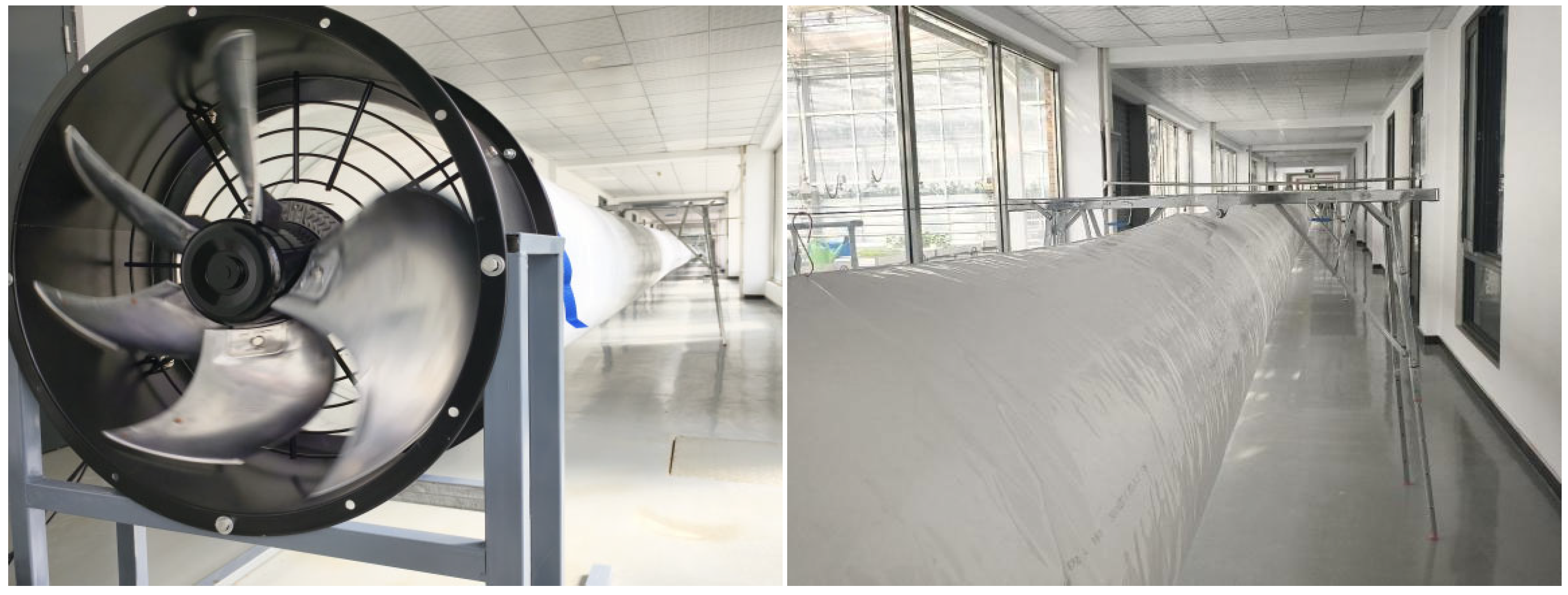
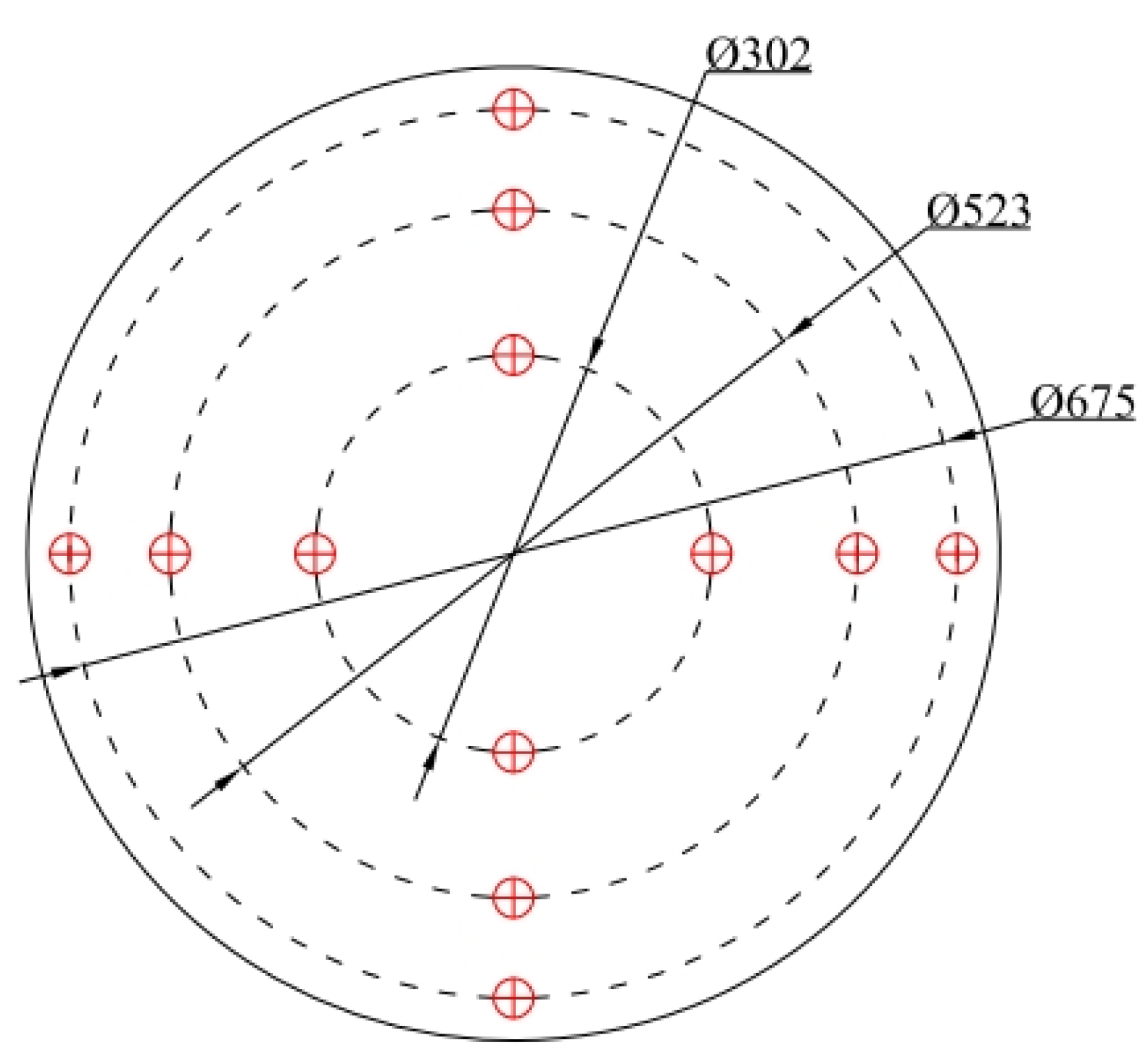
2.1. Physical Model Construction

We constructed a 1:1 scale three-dimensional geometric model of a perforated air duct using SolidWorks 2024 (Figure 1). The duct measures 100 m in length, 0.74 m in diameter, and has a wall thickness of 0.2 mm. Four rows of outlet holes are uniformly distributed along the axial direction at the 4, 5, 7, and 8 o’clock positions; each hole is 8 mm in hole diameter, with 30 mm spacing between holes. The computational fluid domain was defined with its origin (x = 0, y = 0, z = 0) at the centroid of the duct inlet cross-section, and the positive x-axis aligned with the airflow direction.

2.2. CFD Model Construction

2.2.1. Mathematical Model

The air within the semi-closed greenhouse was modeled as a steady, incompressible medium. The coupled mass and heat transfer processes were governed by the conservation equations of mass, momentum, and energy, which can be collectively expressed using the generalized transport equation (Equation (1)):

$${\displaystyle \frac{\partial (\rho \phi )}{\partial t}}+{\displaystyle \frac{\partial (\rho u_j)}{\partial x_j}}={\displaystyle \frac{\partial }{\partial x_j}}({\mathrm{\Gamma }}_{\phi }{\displaystyle \frac{\partial \phi }{\partial x_j}})+S_{\phi }$$

(1)

where $\phi$ is the generalized variable; $\rho$ denotes the density (kg·m⁻³); $u_j$ represents the velocity vector (m·s⁻¹); ${\mathrm{\Gamma }}_{\phi }$ stands for the generalized diffusion coefficient; and $S_{\phi }$ indicates the source term.

When solving the governing equations for duct flow fields, distinct physical parameter expressions are derived according to the target variable Φ. By specifying initial conditions and physical boundary constraints, the fundamental governing equations can be solved. The resulting expressions for each term in the general transport equation are systematically summarized in

Table 1. The various expressions of the general governing equations.

governing equation	$\phi$	${\Gamma }_{\phi }$	S
mass conservation	1	0	0
momentum equation	$u_j$	$\mu$	$-{\displaystyle \frac{\partial \rho }{\partial x_j}}+S_j$
energy equation	T	$k/C_p$	$S_t$

.

This study models steady incompressible turbulent flow using the k-ω SST turbulence model for its superior handling of perforated duct flows. The model combines k-ε stability in core regions with k-ω precision near walls (y⁺ < 5), enhanced by the following: (1) Bradshaw’s assumption enhances adverse pressure gradient predictions by limiting eddy viscosity ${\mu }_t$ via shear stress–turbulent kinetic energy proportionality in boundary layers. (2) Cross-diffusion improves separation prediction. (3) Automatic zone transition via blending functions. These features enable the accurate simulation of adverse pressure gradients and separation zones critical for greenhouse ventilation ducts [24].

$$\rho {\displaystyle \frac{\partial k}{\partial t}}+\rho u_i{\displaystyle \frac{\partial k}{\partial x_i}}={\tau }_{ij}{\displaystyle \frac{\partial u_i}{\partial x_j}}-{\beta }^{*}\rho \omega k+{\displaystyle \frac{\partial }{\partial x_j}}\left[\left(\mu +{\sigma }_k{\mu }_t\right){\displaystyle \frac{\partial k}{\partial x_j}}\right]$$

(2)

$$\rho {\displaystyle \frac{\partial \omega }{\partial t}}+\rho u_i{\displaystyle \frac{\partial \omega }{\partial x_i}}={\displaystyle \frac{\gamma }{v_t}}{\tau }_{ij}{\displaystyle \frac{\partial u_i}{\partial x_j}}-\beta \rho {\omega }^2+{\displaystyle \frac{\partial }{\partial x_j}}\left[\left(\mu +{\sigma }_{\omega }{\mu }_t\right){\displaystyle \frac{\partial \omega }{\partial x_j}}\right]+2\left(1-F_1\right)\rho {\sigma }_{\omega 2}{\displaystyle \frac{1}{\omega }}{\displaystyle \frac{\partial k}{\partial x_j}}{\displaystyle \frac{\partial \omega }{\partial x_j}}$$

(3)

$${\mu }_t={\displaystyle \frac{\rho a_{1}k}{\max \left(a_1\omega ;S{F}_2\right)}}$$

(4)

In the SST model, the strain rate invariant S replaces vorticity, while blending functions F1 and F2 automatically transition between k-ω and k-ε zones.

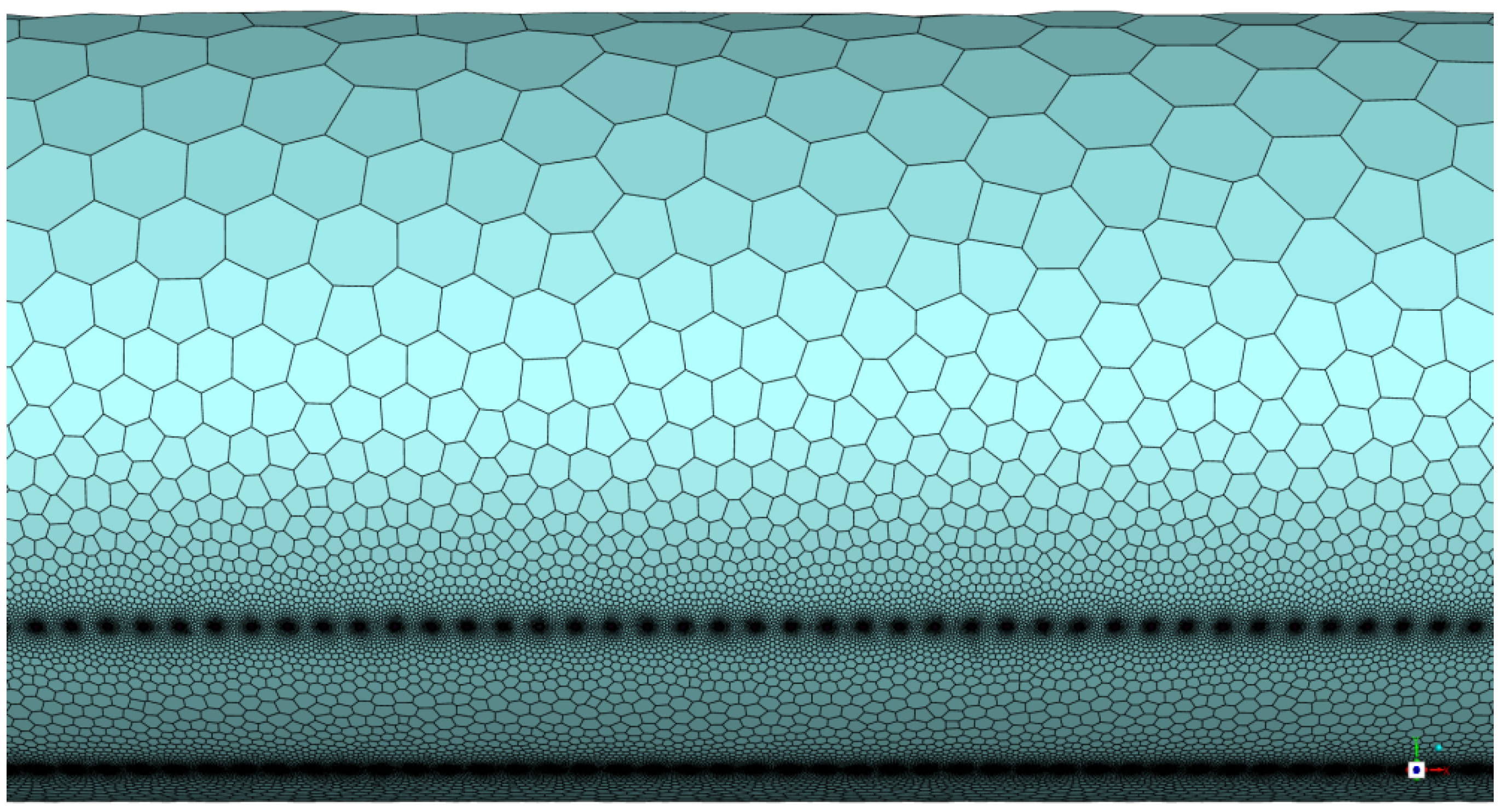
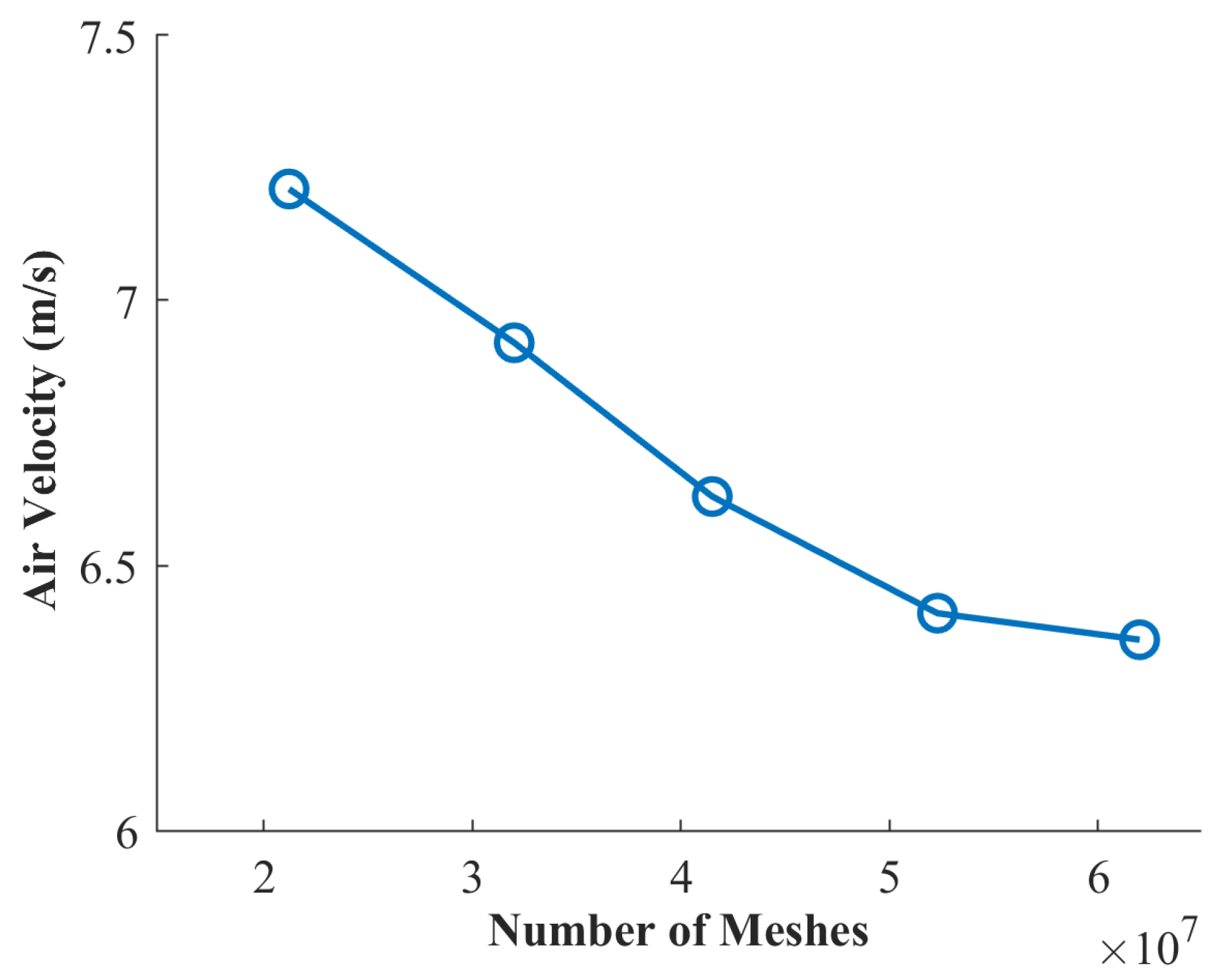
2.2.2. Mesh Generation and Independence Verification

The computational domain was discretized using the polyhedral meshing technique in Fluent Meshing, with pore-level mesh refinement applied specifically at the air tuyere regions to enhance simulation accuracy. The right-side view of the cross-section at 50 m from the inlet, as shown in Figure 2, clearly demonstrates the circumferential mesh refinement strategy.

To ensure the reliability of the simulation results, a grid independence test was performed using grid sizes ranging from 20 to 60 million. The evaluation metric was the average velocity (V) at a cross-section 50 m from the air supply outlet. Computational efficiency was quantified via single-run CPU times on an Intel^® Xeon^® Gold 6248R CPU@3.0GHz, with mesh resolutions requiring 2.1 h (20 M), 3.4 h (30 M), 4.3 h (40 M), 5.1 h (50 M), and 6.8 h (60 M). Results indicated negligible changes (<0.3%) beyond 50 million elements (Figure 3). Consequently, a 50-million-element mesh was adopted for subsequent simulations, optimizing computational efficiency while maintaining solution accuracy.

2.2.3. Boundary Conditions and Solver Settings

The fan inlet was set as a velocity inlet with an initial temperature of 22 °C. The opposite end of the duct was sealed, and the perforated outlets were defined as pressure outlets with a gauge pressure of 0 Pa. The duct surface was specified as a no-slip wall at a constant temperature of 32 °C.

A steady-state heat transfer model was adopted, and the SIMPLEC algorithm was used for pressure–velocity coupling. The least-squares method was applied to the gradient term for spatial discretization, while second-order upwind schemes were employed for the momentum, energy, and turbulence kinetic energy equations. Residual tolerances were set to 10⁻⁶ for the energy equation and 10⁻³ for the momentum and viscous terms.

2.3. Parameter Design

2.3.1. Velocity Design

According to ANSI/ASAE EP406.4 [25], the required ventilation rate was determined by excluding excess heat.

$$q_b={\displaystyle \frac{a\tau E(1-\gamma )(1-\beta )-{\displaystyle \sum _{k=1}^n{K}_k{A}_{gk}(t_i-t_o)/A_s}}{c_p{\rho }_a(t_p-t_j)}}$$

(5)

where $q_b$ represents the required ventilation rate (${\mathrm{m}}^3\cdot {\mathrm{s}}^{-1}$), $\alpha$ is the heat-absorbing area correction coefficient of the greenhouse, set to $\alpha$ = 1.0; $\tau$ is the solar radiation transmittance of the covering layer; $E$ is the outdoor horizontal-plane total solar irradiance (W m⁻²; 1037 W m⁻² at 40° N in summer); $\gamma$ is the indoor solar radiation reflectance (taken as 0.1); $\beta$ is the ratio of latent heat of evaporation to absorbed solar radiation (taken as 0.7); $K_k$ is the heat-transfer coefficient of the nth covering component (W m⁻² K⁻¹); $A_{gk}$ is the area of the kth covering component (m²); $t_i$ is the indoor air dry-bulb temperature (°C; chosen as 28 °C); $t_o$ is the outdoor mean temperature (°C; taken as 35 °C); $A_s$ is the greenhouse ground area (m²; equal to span width × length, here 8 m × 100 m); $c_p$ is the specific heat of air at constant pressure (1030 J kg⁻¹ K⁻¹); ${\rho }_a$ is the density of exhaust air (kg m⁻³); and $t_p$ is the exhaust air temperature (approximated as $t_o$).

The temperature of air entering through the wet-pad $t_j$ was calculated by

$$t_j=t_0-\mu \left(t_0-t_s\right)$$

(6)

where $\mu$ is the wet-pad heat exchange efficiency (taken as 0.8) and $t_s$ is the wet-bulb temperature before the pad (taken as 26.4 °C).

Because summer ventilation in semi-closed greenhouses often involves opening the sunshade net, which reduces incoming solar radiation by reflection and scattering, the midday transmittance can be expressed as

$$\tau ={\tau }_0\left(1-w_1\right)\left(1-w_2\right)\left(1-w_3\right)$$

(7)

where ${\tau }_0$ is the solar radiation transmittance of the clean covering material, taken as 88% in this study; and w₁, w₂, w₃ represent transmittance losses due to structural shading, shading net shading rate, and dust/water droplet contamination, with values of 0.05, 0.4, and 0.1, respectively.

The ventilation rate per duct $Q$ is

$$Q={\displaystyle \frac{q_b{A}_s}{n_b}}$$

(8)

In the formula, $n_b$ represents the number of air ducts (dimensionless), assigned a value of 5. From Equations (1)–(8), each perforated outlet was designed for Q = 3.36 m³ s⁻¹.

The relationship between fan-inlet velocity and flow rate $V$ is

$$V={\displaystyle \frac{4Q}{\pi D^2}}$$

(9)

where duct diameter D = 0.74 m.

To maintain a cylindrical shape and stable airflow in a perforated polyethylene duct, the fan must supply an initial static pressure of 30–40 Pa. The minimum pressure to overcome frictional losses was estimated via the Darcy–Weisbach equation [26]

$$V_{\min }=\sqrt{{\displaystyle \frac{2P_{o}D}{\lambda L\rho }}}$$

(10)

where $P_o$ is the initial static pressure (30 Pa), and $\lambda$ denotes the friction factor (0.02 for polyethylene ducts).

The calculation of Equations (8)–(10) yields a velocity range of 4–8 m/s, with discrete design values constrained by fan speed increments.

2.3.2. Duct Parameter Design

External air significantly regulates temperature, humidity, and CO₂ concentration in the greenhouse crop zone; if air velocity in the crop zone falls below 0.1 m/s, crop transpiration decreases; if it exceeds 0.5 m/s, CO₂ uptake is impaired. The outlet-hole air velocity influences jet penetration: the farther from the hole, the lower the velocity. Ducts should be designed so that, during ventilation, air velocity near the crop zone remains between 0.1 and 0.5 m/s [27]. According to the equation, the outlet-hole air velocity $V_i$ is given by [14].

$$V_i={\displaystyle \frac{2x{V}_x}{dK\sqrt{\pi C_{di}}}}$$

(11)

where $V_i$ is the outlet-hole air velocity (m s⁻¹); $K$ is a constant (5.7); $V_x$ is the air velocity at distance x from the hole (m s⁻¹); $x$ is the distance from the outlet to the crop zone (1.0 m); and $C_{di}$ is the discharge coefficient of the outlet hole (0.64).

The airflow velocity $V_i$ through outlet holes is a function of the static pressure $P_i$ inside the duct, given by:

$$V_i=\sqrt{{\displaystyle \frac{2P_i}{\rho }}}$$

(12)

The hole diameter $d$ is obtained by combining Equations (11) and (12):

$$d={\displaystyle \frac{x{V}_x}{K}}\sqrt{{\displaystyle \frac{2\rho }{\pi P_i{C}_{di}}}}$$

(13)

The design of the outlet holes also took manufacturing feasibility into account, yielding a hole diameter of 6–10 mm.

The hole spacing $L_d$ was calculated from the number of holes $N$ and the number of outlet-hole rows per side $L_b$:

$$L_d={\displaystyle \frac{2L_{b}L}{N}}$$

(14)

where $L_b$ represents the number of hole diameter rows per duct side, set to 2 rows in this study. Notably, N must be an exact integer multiple of $L_b$ to ensure symmetrical airflow distribution.

The number of holes per duct (N) is:

$$N={\displaystyle \frac{4Q}{V_i\pi d^2}}$$

(15)

Based on Equations (11)–(15), the hole spacing corresponding to various hole diameters was calculated, as presented in

Table 2. Duct design parameters.

Hole diameter (mm)	6	8	10
Theoretical spacing (mm)	13.3~66.7	17.8~88.9	22.2~111.0

. The theoretical spacing range for hole diameters d = 6–10 mm is 13.3–111.0 mm. Airflow organization studies require that the spacing satisfies S ≥ 3 d (where S is the hole spacing and d is the hole diameter) [28]. Considering manufacturing precision, the actual hole spacing was controlled within 30–70 mm.

2.3.3. Power Consumption Calculation

The fan power is calculated based on the air volume and pressure (total system resistance) handled by each fan unit. The specific calculation method is as follows:

$$E={\displaystyle \frac{Q_a{P}_{tot}}{3600\eta {\eta }_m}}$$

(16)

where E is electrical power of the fan (kW); $Q_a$ is actual operational air volume (m³/h); ΔP is pressure (Pa); $\eta$ is fan efficiency (typically 0.75–0.85 for axial fans; ${\eta }_m$ is mechanical transmission efficiency (taken as 1.0 for direct motor coupling).

The wind pressure $P_{tot}$ representing the sum of frictional and local resistances is

$$P_{tot}=K_p({\displaystyle \frac{\lambda L}{D}}\cdot {\displaystyle \frac{\rho {v_m}^2}{2}}+\zeta {\displaystyle \frac{\rho {v_m}^2}{2}})$$

(17)

where $K_p$ is the wind pressure loss correction coefficient, with a value of 1.2 for EC fans; $v_m$ is the average air velocity in the perforated duct; and ζ is local resistance coefficient.

The power consumption $C$ of the ventilation system is determined by the actual operating power and runtime of all system fans.

$$C=Et$$

(18)

where $C$ is power consumption of the ventilation system ($\mathrm{KW}\cdot \mathrm{h}$); and t is daily high-speed operational duration. As the system operates exclusively at high wind speeds during the daytime under summer conditions, t = 10 h/day represents the cumulative high-intensity runtime period.

2.4. Response Surface Analysis

In the design of a long-distance air-delivery system for a semi-closed greenhouse, once the duct diameter and number of hole rows are fixed, the key variables affecting airflow distribution and energy consumption are air velocity, hole diameter, and hole spacing (parameter ranges are given in Section 2.3.1 and Section 2.3.2). Key design tradeoffs emerge: oversized perforations or spacing impair airflow uniformity, whereas undersized configurations induce excessive pressure buildup and energy penalties [16]. Similarly, air velocity requires optimization—elevated levels risk pressure violations, while diminished rates compromise ventilation efficacy Therefore, we optimize three objectives: velocity variation coefficient (CV-v), temperature variation coefficient (CV-t), and pressure loss (ΔP).

CV-v serves as a spatial uniformity metric for air velocity distributions within critical agricultural planes, particularly at crop canopy elevation. Minimizing CV-v constitutes a primary optimization objective because consistent velocity distribution is essential for maintaining homogeneous crop growth environments in greenhouses. Non-uniform airflow causes localized ventilation deficiencies (increasing risks of humidity-related diseases and heat accumulation) or excessive velocities (inducing physical damage), ultimately disrupting transpiration rates, photosynthetic efficiency, and growth quality uniformity across cultivation areas [27,29]. CV-v is calculated as the ratio of standard deviation to mean velocity, where higher values indicate poorer spatial homogeneity:

$$CV\text{-}v={\displaystyle \frac{\sqrt{\frac{1}{n-1}{{\displaystyle \sum }}_{i=1}^n{\left(v_i-\overline{v}\right)}^2}}{\overline{v}}}$$

(19)

where $v_i$ represents the airflow velocity at each outlet (m/s), and $\overline{v}$ denotes the average airflow velocity across all outlets (m/s).

The CV-t metric quantifies the spatial homogeneity of temperature distribution. Minimizing CV-t is critical to ensure crop physiological synchrony: Localized high- or low-temperature stress inhibits photosynthetic efficiency, leading to asynchronous development and yield reduction [30]. Temperature heterogeneity also forces environmental control systems to over-regulate specific zones, substantially increasing energy consumption. CV-t optimization directly correlates with enhanced crop quality and improved energy efficiency.

$$CV\text{-}t={\displaystyle \frac{\sqrt{\frac{1}{n-1}{{\displaystyle \sum }}_{i=1}^n{\left(t_i-\overline{t}\right)}^2}}{\overline{t}}}$$

(20)

where $t_i$ denotes the temperature at each outlet and $\overline{t}$ is the mean temperature of all outlets (°C).

ΔP characterizes the total pressure loss across ventilation systems. Minimizing ΔP represents a critical economic objective for reducing energy consumption: Fan power scales linearly with ΔP, making it a primary engineering parameter influencing the operational economy of continuously operated agricultural facilities [4]. ΔP is calculated as the differential between inlet and outlet total pressures, and its optimization directly governs system sustainability and operational costs.

$$\Delta P=P_a-P_b$$

(21)

where $P_a$ and $P_b$ are the total pressures (Pa) at the duct inlet and outlet.

To enable efficient parameter optimization, a three-factor, three-level Box–Behnken experimental design was adopted to construct a response surface model. This strategy reduced experimental efforts while systematically probing interactions among air velocity, hole diameter, and hole spacing. Surrogate models correlating these parameters with the objectives (CV-v, ΔP and CV-t) were developed. Details of the experimental factors and level settings are provided in

Table 3. Factor level.

	−1	0	1
A: Velocity (m/s)	4	6	8
B: Hole space (mm)	30	50	70
C: Hole diameter (mm)	6	8	10

.

2.5. Multi-Objective Optimization

Multi-objective optimization problems (MOPs) require balancing conflicting objectives. This study utilizes the second-generation non-dominated sorting genetic algorithm (NSGA-II) as the core solver [31]. By leveraging its fast non-dominated sorting and crowding-distance mechanisms, NSGA-II efficiently identifies Pareto-optimal solutions while maintaining population diversity.

2.5.1. NSGA-II

Direct CFD-NSGA-II coupling was computationally prohibitive (10⁴ h). Instead, the RSM-derived quadratic polynomials enabled computationally tractable optimization while rigorously capturing nonlinear parameter interactions. This approach balanced accuracy with feasibility given the high-fidelity model constraints. To optimize parameters of a semi-closed greenhouse supply air system, a hybrid framework integrating a response surface methodology (RSM) and NSGA-II is proposed. First, RSM constructs quadratic surrogate models for CV-v, ΔP, and CV-t, significantly reducing computational costs. Subsequently, NSGA-II iteratively minimizes these objectives (CV-v, ΔP, and CV-t) in parallel.

$$f(1)=\mathit{Minimize}(CV\text{-}v)$$

(22)

$$f(2)=\mathit{Minimize}(\Delta P)$$

(23)

$$f(3)=\mathit{Minimize}(CV\text{-}t)$$

(24)

To ensure engineering feasibility, the static pressure at the duct inlet was maintained at 30 Pa, thereby ensuring structural stability and preserving the cylindrical form of the polyethylene air duct. The average static pressure at the cross-section 20 m downstream of the inlet ($P_o$) was adopted as the monitoring threshold to circumvent turbulent fluctuations in the inlet region.

The NSGA-II parameters were determined through rigorous sensitivity analysis: population size was varied from 100 to 300 and generations from 200 to 400, establishing a parameter matrix to quantify convergence performance (hypervolume) and computational time.

In this study, the hypervolume (HV) metric is selected to evaluate the performance of the multi-objective optimization algorithm. The hypervolume simultaneously assesses both convergence and diversity of solutions [32]. A higher HV value indicates superior performance in convergence and diversity. The hypervolume is formally defined as follows [33]:

$$HV(S)=VOL(\underset{s\in S}{\cup })\left[{\lambda }_1\left(s\right),Z_1^r\right]\times \dots \times \left[{\lambda }_m\left(s\right),Z_m^r\right]$$

(25)

where VOL is the Lebesgue measure; m is the number of objectives; $Z^r=Z_1^r\dots Z_m^r$ is a reference point in the target space.

2.5.2. Decision-Making Via Entropy-Weighted TOPSIS

To identify the globally optimal design from the Pareto front, the entropy-weighted TOPSIS (Technique for Order Preference by Similarity to Ideal Solution) method was ap-plied. This approach eliminates subjective bias in weight assignment by quantifying the intrinsic information entropy of each objective. Subsequently, TOPSIS identified the optimal solution by (1) normalizing the decision matrix; (2) applying entropy-derived weights; (3) computing Euclidean distances to positive ideal (Di+) and negative ideal (Di-) solutions; (4) calculating relative closeness (Ci). This method ensures objective balance between airflow uniformity (CV-v), energy efficiency (ΔP), and thermal homogeneity (CV-t). For full methodology, see [34].

2.6. Data Acquisition

2.6.1. Test Conditions

Duct performance tests were conducted on 8–10 June 2025, in Lang-fang City, Hebei Province, China. The test duct was positioned at the center of the corridor of a multi-span greenhouse, with its bottom edge 20 cm above the ground. This study also evaluated the duct’s thermal insulation performance through a control cooling experiment using early morning ambient air as the cooling source. All experiments were conducted at early morning (5:00–7:00) to establish a stable temperature difference. An axial fan was placed outside the corridor, and the duct region was physically separated from the fan compartment by a 0.2 mm polyethylene film barrier. This configuration prevented direct thermal interference while maintaining the required airflow characteristics.

Figure 4 shows the full-scale (1:1) duct rig used for testing. Experimental validation was performed using a wind tunnel with physically identical perforations (8 mm diameter, 30 mm spacing) to the numerical model under 8 m/s flow conditions. This high-velocity, dense-spacing scenario provides stringent verification of turbulence modeling accuracy. The duct’s polyethylene film was lightweight, deformation-resistant, and easy to install. An EC fan at the inlet controlled air velocity via speed adjustment. Downstream ventilation holes were fitted with a damper, which in this study kept them closed.

Wind speed attenuation tests were conducted on 15 June 2025 at a semi-closed greenhouse facility in Qinhuangdao, China, to validate Equation (11). The experimental greenhouse featured a single-span width of 9 m and total length of 120 m, with air tubes arranged at 1.8 m intervals. All tubes were in-stalled 20 cm above ground level and maintained identical specifications to the Langfang reference tubes: nominal diameter Ø = 0.74 m, with uniformly distributed 8 mm perforations at 30 mm spacing intervals (Figure 5).

2.6.2. Test Method

The equal-area annular method determined wind velocity and static pressure in the duct. Every 5 m along the duct length constituted one measurement section; for the 100 m duct, there were 20 sections. Each section was divided into three equal-area concentric rings, and 10 measurement points were arranged on each cross-section, as shown in Figure 6. The Formula (10) calculated the distance ($R_i$) from the center to each point on the concentric rings:

$$R_i=R_0\sqrt{{\displaystyle \frac{2i-1}{2n}}}$$

(26)

where $R_i$ is the distance from the duct center to point i-th (mm); $R_0$ is the duct radius (mm); $i$ is the sequence number of the concentric ring; and $n$ is the number of rings on the duct cross-section (here n = 3)

Outlet wind speed decay was measured horizontally using the hot-wire anemometer, with readings taken at 10 cm intervals across 10 points. Triplicate measurements at each point ensured statistical robustness, with final values derived from arithmetic means.

A variable-speed EC fan (GSG-EC-710-A-03, Beijing GroSens Environmental Engineering Technology Co., Ltd., Beijing, China) with adjustable rotational speed (400–1800 r/min via frequency converter) was employed, delivering a maximum airflow of 20,000 m³/h. In-pipe airflow velocity, temperature, and pressure were measured using a multifunctional detection system (YIOU DP7000A, Shanghai Yiou Instrument & Equipment Co., Ltd., Shanghai, China), with ranges of 0–500 Pa, 0–30 m/sand—50–100 °C, ±0.5% accuracy, and a 40 cm probe. Exit airflow velocity was quantified with a hot-wire anemometer (Testo 405i, Testo SE & Co. KGaA, Lenzkirch, Germany) with a resolution of ±0.1 m/s velocity.

To ensure experimental accuracy, this study quantifies measurement results using uncertainty analysis. The expanded uncertainty of wind speed, total pressure, and temperature measurements is calculated by combining Type A (statistical) and Type B (non-statistical) uncertainty components. Type A uncertainty arises from repeated measurements, while Type B includes instrument calibration errors, positioning deviations, and technical specifications. The specific testing procedure is described in Appendix A.

3. Results and Discussion

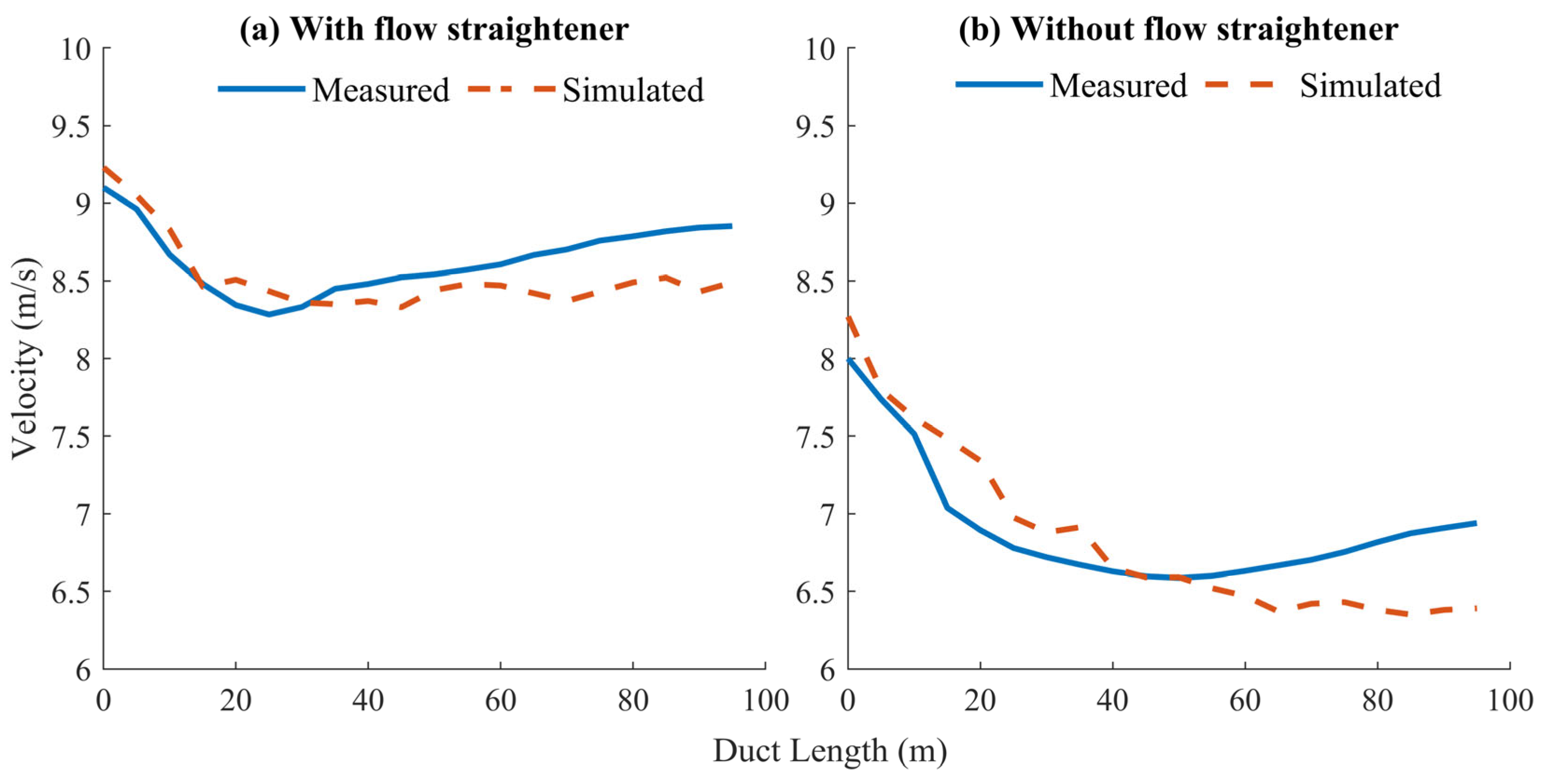
3.1. Model Validation

Figure 7a presents the flow velocities measured at each point inside the duct. The results showed that, due to frictional resistance, velocity decreased along the duct from approximately 8 m/s to 0 m/s. Experimental measurements agreed with theoretical CFD predictions: the absolute deviation between simulated and measured velocities ranged from 0.01 to 0.49 m/s, with an average relative error of 8.57%. The temperature rose along the duct axis from about 22 °C to 27 °C; the absolute deviation between simulated and measured temperatures was 0.15–0.39 °C, with an average relative error of 2.28%. These findings indicated that the CFD model accurately reflected actual conditions and was thus valid for data analysis and subsequent simulations.

Figure 7b compared static and dynamic pressures at different duct sections; theoretical calculations and numerical simulations matched experimental results within 5 Pa. The relative errors of numerical simulation versus experimental data were 3.86% and 8.54%, respectively, demonstrating that both approaches can accurately predict pressure distribution in perforated ducts.

It can be seen from Appendix A that the expanded uncertainties for wind speed, total pressure, and temperature are 0.80 m/s, 6.44 Pa, and 0.46 °C, respectively. These results confirm that the measurement precision falls within an acceptable range, thus supporting the reliability of the experimental data.

Figure 8 compares simulated and experimental air velocity distributions downstream of the outlet in a semi-closed greenhouse, demonstrating excellent model agreement (R² = 0.973). The observed discrepancy at 20 cm from the outlet is operationally negligible, since (1) this proximal zone precedes crop canopy coverage where airflow has minimal agronomic impact; (2) downward-oriented outlet jets create localized low-velocity regions; and (3) critical crop-growing areas (≥0.5 m) maintain velocities within the optimal 0.1–0.5 m/s threshold.

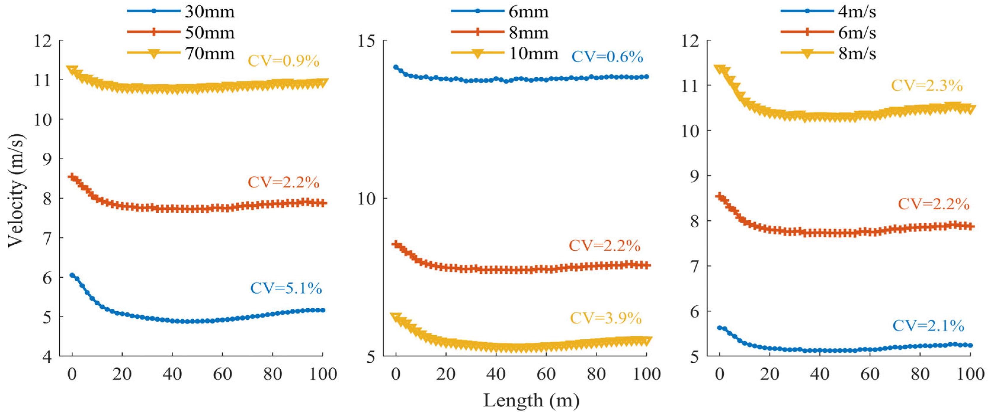
3.2. Single-Factor Analysis

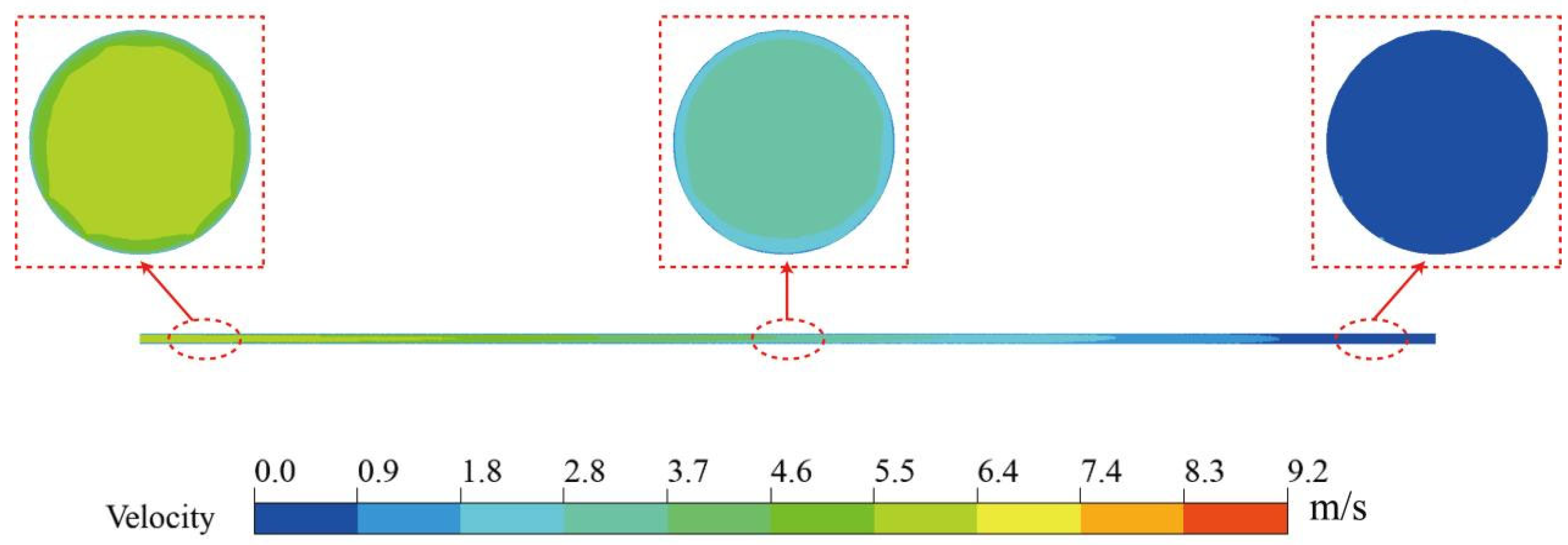
3.2.1. Velocity Field

To investigate how perforations affect the flow-field distribution inside the duct, we conducted a simulation of a duct with a hole diameter of 8 mm, hole spacing of 50 mm, and an inlet velocity of 6 m/s. The horizontal velocity distribution was analyzed via velocity-field contours (Figure 9). The results show that the velocity along the flow direction decreases linearly and that the internal velocity distribution is symmetric about the centerline. Notably, owing to end-closure–induced turbulence at the tail, the distribution becomes asymmetric. Therefore, adding perforations near the duct outlet could enhance end-region air delivery and reduce turbulence.

A comparison of velocity distributions at three representative sections—initial (5 m), mid-span (50 m), and terminal (95 m)—reveals that the boundary layer thins noticeably near the four lower holes. However, from an overall perspective, local perforations have little effect on the duct’s bulk flow field. Over most of the cross-section, the gas flows steadily at a uniform speed. Near each perforation, the flow-field characteristics conform to the typical behavior of a pressure-outlet boundary condition. Exit velocities reached a maximum of 9.2 m/s, representing a 53.3% boost over the inlet speed. The three-dimensional velocity contours reveal that the maximum speed occurs at the outlet region, then decays toward the midsection, while a distinct low-speed zone forms along the duct periphery.

As shown in Figure 10, this study uses CFD simulations to elucidate the regulatory behavior of perforated ducts under various parameters. Under the baseline condition of 8 mm hole diameter, 50 mm spacing, and 6 m/s inlet speed, the region from 0 to 40 m downstream of the inlet exhibits a rapid velocity drop—10.3% lower than the initial value at 40 m—due to turbulence effects. Thereafter, owing to static-pressure recovery, velocity shows only a slight rebound of 2.2% between 40 m and 100 m. This indicates that the turbulence-dominated zone exerts a decisive influence on overall velocity decay.

Parameter sensitivity analysis indicates that increasing hole spacing from 30 mm to 70 mm raises the mean exit velocity by 113% and significantly improves flow uniformity, with the coefficient of variation decreasing from 5.1% to 0.9%. This phenomenon exhibits strong concordance with the Suhardiyanto and Matsuoka [35] theoretical model. Their research demonstrated that increasing orifice spacing from 6 cm to 10 cm elevates airflow uniformity from 96% to 99%. Our study further establishes that this wide-spacing strategy delivers significantly enhanced benefits in extended duct systems (100 m versus their 10 m prototype). Conversely, reducing orifice diameter from 10 mm to 6 mm increased outlet velocity by 252% but raised the coefficient of variation (CV) from 0.6% to 3.9%, indicating significantly compromised uniformity. This outcome corroborates the key finding of El Moueddeb et al. [36] that enlarging orifice size intensifies flow nonuniformity at the outlet—a phenomenon fundamentally attributed to elevated static pressure at the duct’s sealed end caused by increased orifice-to-duct area ratio, which disrupts balanced flow distribution. Increasing the inlet speed from 4 m/s to 8 m/s boosts exit velocity by 104% but weakens uniformity. These findings demonstrate that decreasing the hole-to-spacing ratio can simultaneously optimize velocity and uniformity.

To mitigate the turbulence-induced velocity decay identified in Figure 10, a flow straightener was installed upstream of the intake duct (Figure A1). Experimental comparisons with and without the device demonstrated that its installation significantly enhanced ventilation performance: the average outlet velocity increased from 6.9 m/s (coefficient of variation, CV = 5.6%) to 8.6 m/s (CV = 2.2%). This optimization achieved a 60.7% reduction in the velocity variation coefficient, while stability improved through a 72.2% decrease in velocity decay magnitude (from 1.8 m/s to 0.5 m/s) and a reduction in decay rate from 20.7% to 5.8% (Figure A2). Consequently, this study confirms that flow straighteners are essential for ventilation systems, as they mitigate airflow separation at the inlet while enhancing duct airflow delivery efficiency. (For detailed data, see Appendix B).

3.2.2. Pressure Field

Axial pressure distribution along the ventilation duct (Figure 11). Pressure decreases from 60.0 Pa at the inlet to 43.8 Pa at the outlet, with a 26.9% total reduction. Notably, the pressure gradient is steeper in the initial segment (0–30 m: 0.38 Pa/m) than in the downstream section (70–100 m: 0.08 Pa/m)

Based on an analysis of total-pressure characteristics in a semi-closed greenhouse positive-pressure duct system, this study introduces the concept of “pressure-recovery length”. It systematically quantifies its dependence on hole spacing, hole diameter, and inlet velocity (Figure 12). Hole spacing and pressure-recovery length are strongly negatively correlated: when spacing increases from 30 mm to 70 mm, the recovery length decreases from 40 m to 25 m because closer holes intensify spatial interference between adjacent jets, raise turbulence intensity, and accelerate energy dissipation [37]. Hole diameter and recovery length are positively correlated: enlarging hole diameter from 6 mm to 10 mm extends the recovery length from 30 m to 42 m, since a larger hole diameter increases the mass flow per hole, enhances shear-mixing among multiple jets, and delays pressure stabilization. Varying inlet velocity between 4 m/s and 8 m/s alters the recovery length by less than 5%, indicating that inertia dominates flow behavior and viscous effects are negligible. In practice, combining small hole diameters with wide spacing can reduce the pressure-recovery length to 25–30 m.

Further analysis reveals synergistic interactions between total pressure (P) and pressure loss (ΔP) under structural parameter adjustments. This synergy is critical for energy efficiency and is analyzed as follows: Reducing hole spacing from 70 mm to 30 mm decreases P by 78.2% and ΔP by 35.5%, as tighter spacing intensifies multi-jet interference and turbulent dissipation. Similarly, increasing hole diameter from 6 mm to 10 mm reduces P by 85.0% and ΔP by 54.8%, attributable to elevated local flow rates and expanded jet disturbance zones. Velocity variations exert the strongest influence: raising inlet velocity from 4 m/s to 8 m/s amplifies P and ΔP by 297.7% and 298.2%, respectively, underscoring their acute sensitivity to velocity changes in turbulent regimes. These results confirm that combining larger hole diameters with reduced spacing synergistically minimizes system pressure loss [16].

3.2.3. Temperature Field

As shown in Figure 13, the horizontal temperature distribution was quantitatively analyzed using temperature-field contours. The results indicate that the perforated structure markedly influences the temperature-field distribution within the 100 m duct: along the flow direction, the temperature declines sharply from 31.8 °C at the inlet (5 m) to 22.0 °C at the outlet (95 m), a decrease of 31.1%, and vertical temperature stratification intensifies with distance. At mid-span (50 m), the temperature difference between the top and bottom reaches 1.2 °C, expanding to 4.3 °C at the outlet (95 m). In the inlet region, thorough mixing yields a uniform temperature profile, whereas downstream, buoyancy-driven settling and turbulent dissipation cause cooler air to accumulate near the bottom.

Quantitative analysis of Figure 14 revealed a pronounced three-stage pattern in the axial temperature distribution along the duct. In the region 0–20 m downstream of the inlet, the temperature rose rapidly at 0.8 °C m⁻¹, decaying to 0.3 °C m⁻¹ over the mid-section from 20 to 90 m before exhibiting a sharp increase of 1.6 °C m⁻¹ in the terminal 90–100 m segment. This surge was attributed to a thermal-retention effect within the recirculation zone at the duct outlet. The study further showed that orifice hole diameter (6–10 mm) and spacing (30–70 mm) exerted only a weak influence on the exit temperature field, with the maximum temperature difference among different hole diameter–spacing combinations at the same flow speed being merely 0.08 °C and the coefficient of variation in temperature differing by no more than 0.3 percentage points; these findings confirm that orifice geometry does not significantly affect temperature uniformity [35]. By contrast, inlet velocity played a decisive role in thermal regulation: when the flow speed increased from 4 m s⁻¹ to 8 m s⁻¹, the mean outlet temperature dropped by 1.0 °C and the temperature-variation coefficient fell from 5.5% to 4.6%, indicating that higher velocities enhance turbulent mixing and thereby suppress local heat accumulation, achieving improved temperature uniformity.

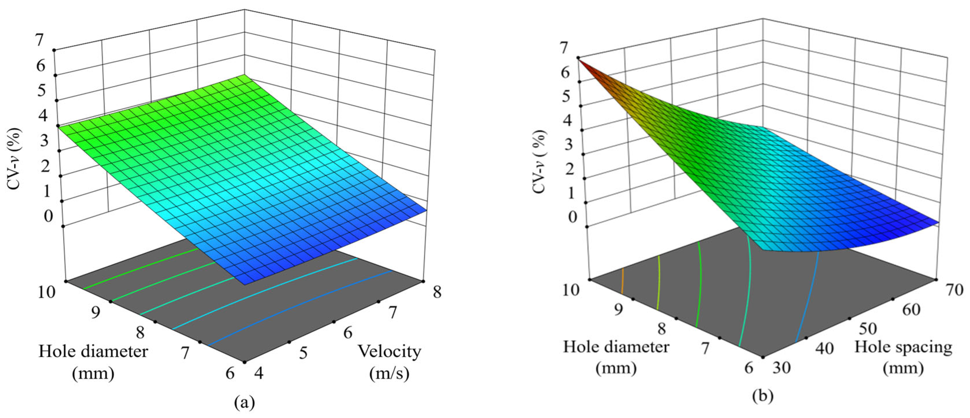
3.3. Response Surface

This study selected the coefficient of variation in velocity (CV-v), pressure loss (ΔP), and the coefficient of variation in temperature (CV-t) as optimization objectives. A three-factor, three-level experimental matrix was constructed using the Box–Behnken central composite design (

Table 4. Analysis of variance (ANOVA) with significance testing.

	Y1 (CV-v)		Y2 (ΔP)		Y3 (CV-t)
	F-Value	F-Value	F-Value	p-Value	F-Value	p-Value
Model	88.25	74.93	50.5	<0.0001	74.93	<0.0001
A	0.5662	659.84	200.05	<0.0001	659.84	<0.0001
B	344.33	1.52	55.67	<0.0001	1.52	0.2576
C	390.57	4.04	112.14	<0.0001	4.04	0.0843
AB	0.0016	1.02	8.06	0.0001	1.02	0.3465
AC	0.0681	0.4124	15.15	<0.0001	0.4124	0.5412
BC	41.02	0.0337	52.65	<0.0001	0.0337	0.8596
A2	0.4131	6.08	0.0946	0.0039	6.08	0.0431
B2	15.51	0.7498	0.8115	0.1244	0.7498	0.4152
C2	0.9058	0.2395	9.6	0.0279	0.2395	0.6395
Lack of Fit	2.39	0.2675	3.0	0.1582	0.2675	0.8463

), and response surface models were developed via Design-Expert 13 software.

Significance analysis (Table 4) showed that terms in the Y₁(CV-v) model were highly significant (p < 0.0001), while the lack-of-fit term was insignificant (p = 0.2069), confirming model validity, controllable error, and high goodness-of-fit (R² = 0.9802). The dominant factors were B, C, the BC interaction term, and the B² term, ranked by influence as C > B > A. The Y₁ regression equation is

$$\begin{array}{l}{Y}_1=2.17+0.0663A-1.63B+1.74C-0.005AB+0.0325AC-0.7975BC\\ +0.078A^2+0.478B^2+0.1155C^2\end{array}$$

(27)

Similarly, the Y₂ (ΔP) model achieved the best fit (R² = 0.9861), with all main effects (A, B, C), quadratic terms (C²), and interaction terms (AB, AC, BC) reaching extreme significance (p < 0.0001). The Y₃ equation is

$$\begin{array}{l}{Y}_2=-51.61056+11.64025A+1.22838B-1.05175C+0.0815AB-1.1175AC\\ -0.208313BC-0.086062A^2+0.002521B^2+0.867062C^2\end{array}$$

(28)

Notably, the Y₃ (CV-t) model demonstrated high significance (p < 0.0001) with an insignificant lack-of-fit term (p = 0.8463), minimal error, and strong predictive accuracy (R² = 0.9765). Key factors were A and the A² term. The Y₃ equation is

$$\begin{array}{l}{Y}_3=7.56962-0.444625A-0.001437B-0.103875C-0.000688AB\\ +0.004375AC+0.000125BC+0.016375A^2+0.000057B^2+0.00325C^2\end{array}$$

(29)

Figure 15 illustrates the influence of key interacting factors on the response variables. As shown in Figure 15a, hole diameter exerts a significantly more substantial effect on CV-v than velocity. At a constant hole diameter, CV-v increases marginally with velocity (by less than 5%). Conversely, under fixed velocity conditions, CV-v rises linearly with larger hole diameters. Additionally, increasing hole spacing reduces CV-v at constant hole diameters, with this decline particularly pronounced for hole diameters exceeding 8 mm (Figure 15b). Smaller hole spacings (<50 mm) amplify the sensitivity of CV-v to hole diameter changes. In contrast, larger spacings (>50 mm) attenuate this effect.

ΔP exhibits multifactor coupling effects (Figure 15c,d). At fixed hole diameters, ΔP increases with velocity, especially for smaller diameters (6–8 mm). Larger diameters intensify pressure loss at high velocities, highlighting a velocity-dependent interaction. Hole spacing significantly modulates the impact of hole diameter on ΔP. For small diameters (6–8 mm), ΔP increases sharply with spacing, but this trend weakens for hole diameters above 10 mm. Conversely, at small spacings (30–50 mm), increasing hole diameter causes a gradual decrease in ΔP, while at large spacings (60–70 mm), the decrease becomes abrupt.

CV-t is predominantly governed by velocity (Figure 15e,f). At fixed hole diameters, CV-t declines rapidly with increasing velocity, with negligible contributions from hole diameter or spacing variations. Notably, maintaining a pressure of P_a ≥ 30 Pa is essential for structural stability, thereby constraining the permissible velocity range.

The study reveals a competing relationship between hole diameter and spacing in governing CV-v and ΔP, whereas velocity primarily dictates CV-t and system stability. An entropy-weight TOPSIS–NSGA-II hybrid algorithm will be employed to identify the optimal balance within the Pareto-optimal set under geometric and fluid-dynamic constraints to achieve multi-objective synergistic optimization.

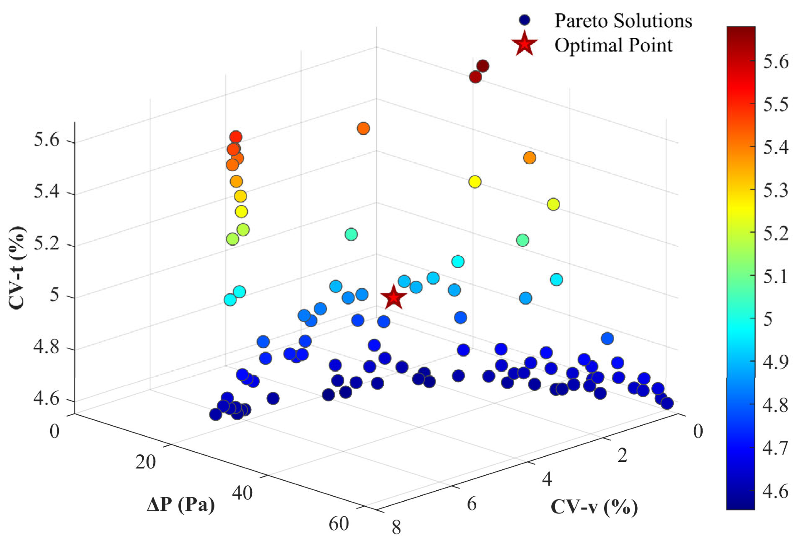
3.4. Parameter Optimization

Figure 16 demonstrates the sensitivity analysis heatmaps for NSGA-II parameters, revealing that a population size of 200 and 300 generations achieves optimal balance be-tween convergence performance and computational efficiency, as higher settings beyond this range yield diminishing HV returns (<1.3% gain) with disproportionate time increases (>32.0%). This configuration was thus selected as the Pareto-optimal trade-off for subsequent optimization studies.

The multi-objective NSGA-II algorithm performed a global search across duct geometry and inlet velocity parameters, generating 80 feasible designs after 300 generations. Figure 17 displays the Pareto front in the objective space, where the x-axis represents CV-v, the y-axis ΔP, and the z-axis CV-t.

An entropy-weighted TOPSIS analysis was applied to the non-dominated solutions. The entropy method assigned objective weights of 0.38 to CV-v, 0.33 to ΔP, and 0.29 to CV-t, indicating velocity uniformity as the highest priority in engineering practice. The Pareto front exhibits a convex shape, with CV-v ranging from 0.32% to 7.87%, ΔP from 0.24 to 59.52 Pa, and CV-t from 4.54% to 5.68%. Based on TOPSIS closeness coefficients, the globally optimal parameter set was identified as follows: hole diameter = 9.02 mm, hole spacing = 64.84 mm, and inlet velocity = 7.03 m/s.

By integrating manufacturing precision considerations, the optimal duct parameters were identified as a 9.0 mm hole diameter, 65 mm spacing, and 7.0 m/s inlet velocity. Comparative analysis with the baseline configuration (8 mm hole diameter, 30 mm spacing, 8 m/s velocity) revealed substantial enhancements (

Table 5. Comparative analysis of optimization results.

Indicator	Pre-Optimization	Post-Optimization	Rate of Change
CV-v (%)	4.64	1.91	−58.83%
ΔP (Pa)	23.7	21.15	−10.76%
CV-t (%)	4.57	4.82	+5.18%
$\mathrm{Power}\mathrm{consumption}(\mathrm{KW}\cdot \mathrm{h})$	7.74	6.39	−17.44%

): the optimized solution achieved a 58.83% reduction in velocity variation coefficient (CV-v), a 10.76% reduction in pressure loss (ΔP), a 5.18% improvement in temperature variation coefficient (CV-t), and a 17.44% reduction in power consumption for the ventilation system. Although this resulted in a slight compromise in temperature uniformity, substantial gains were made in both velocity uniformity and pressure loss reduction. Operational stability was maintained at an inlet static pressure of 72.81 Pa, significantly lower than the 125 Pa typical in conventional greenhouse fabric ducts [38]. The optimized configuration achieves a 41.8% reduction in pressure load compared to conventional systems, while reducing operational costs and improving equipment longevity. The “large-diameter–wide-spacing” strategy balances airflow uniformity, thermal uniformity, and energy efficiency. It mitigates turbulence disturbances, enhances system stability, and provides an innovative solution for greenhouse ventilation systems that optimizes both performance and energy consumption.

4. Conclusions

This study proposes an integrated design framework combining the response surface methodology (RSM) and the NSGA-II multi-objective optimization algorithm to optimize the velocity uniformity coefficient (CV-v), pressure loss (∆P), and temperature variation coefficient (CV-t) in positive-pressure ducts. The interactive effects of hole diameter (6–10 mm), spacing (30–70 mm), and inlet velocity (4–8 m/s) on airflow characteristics were systematically quantified. Model validation demonstrated a mean relative error of 8.57% for velocity and 2.28% for temperature predictions, with static/dynamic pressure deviations below 5 Pa. The response surface model achieved an R² of 0.9831 (p < 0.0001), confirming its reliability.

Key findings include the following: (1) CV-v and pressure-recovery length decreased with larger hole diameters but increased with wider spacing, while ∆P exhibited inverse correlations for hole diameter; temperature uniformity was solely governed by inlet velocity. (2) Sensitivity analysis ranked hole diameter as the dominant parameter, followed by spacing and velocity, with significant hole diameter–spacing interaction effects on airflow uniformity and pressure loss. (3) Multi-objective optimization via entropy-weighted TOPSIS identified the optimal configuration (hole diameter = 9.0 mm, spacing = 65 mm, velocity = 7.0 m/s). This configuration reduced the velocity variation coefficient (CV-v) by 58.83%, decreased pressure loss (ΔP) by 10.76%, improved the temperature variation coefficient (CV-t) by 5.18%, and achieved a 17.44% reduction in ventilation system power consumption—all while stabilizing inlet static pressure at 72.81 Pa. This “large-diameter, wide-spacing” strategy balances flow uniformity and energy efficiency, offering a novel solution for greenhouse ventilation.

Future work will advance duct optimization through a multiscale experimental-theoretical framework, integrating (1) dynamic crop–canopy interactions via coupled transpiration–aerodynamic microclimate modeling; (2) scalability quantification of greenhouse structures through dimension, ventilation opening size, and duct layout parametrization; (3) adaptive control systems linking duct operational parameters to real-time cooling demands under variable solar loading.

References

1. Dijk, M.V.; Morley, T.; Rau, M.L.; Saghai, Y. A meta-analysis of projected global food demand and population at risk of hunger for the period 2010–2050. Nat. Food 2021, 2, 494–501. [Google Scholar] [CrossRef] [PubMed]
2. Shen, Y.; Wei, R.; Xu, L. Energy consumption prediction of a greenhouse and optimization of daily average temperature. Energies 2018, 11, 65. [Google Scholar] [CrossRef]
3. Liu, J.; Li, X.; Wang, C.D.; Zheng, G.; Zhang, T.Z. Design and experiment of the positive pressure ventilation cooling system in glass multi-span greenhouse. J. Chin. Agric. Univ. 2020, 25, 152–162. [Google Scholar] [CrossRef]
4. Sapounas, A.; Katsoulas, N.; Slager, B.; Bezemer, R.; Lelieveld, C. Design, control, and performance aspects of semi-closed greenhouses. Agronomy 2020, 10, 1739. [Google Scholar] [CrossRef]
5. Park, M.-L.; Jeong, J.-W. Review of semi-closed greenhouse previous studies and required technology analysis for improving energy efficiency. KIEAE J. 2022, 22, 21–27. [Google Scholar] [CrossRef]
6. Sannan, S.; Jerca, I.O.; Badulescu, L.A. A CFD study of the fluid flow through air distribution hoses in a greenhouse. Chem. Eng. Trans. 2023, 100, 385–390. [Google Scholar] [CrossRef]
7. Tadj, N.; Nahal, M.A.; Constantinos, K.; Draoui, B. CFD simulation of heating greenhouse using a perforated polyethylene ducts. Int. J. Eng. Syst. Model. Simul. 2017, 9, 3–11. [Google Scholar] [CrossRef]
8. Pardo-Pina, S.; Ferrández-Pastor, J.; Rodríguez, F.; Cámara-Zapata, J. Analysis of an evaporative cooling pad connected to an air distribution system of perforated polyethylene tubes in a greenhouse. Agronomy 2024, 14, 1187. [Google Scholar] [CrossRef]
9. Lu, X.Y.; Yu, C.J. Simulation and experimental study of the air distribution characteristics of large-span film air duct in greenhouses. Trans. Chin. Soc. Agric. Eng. 2024, 40, 204–211. [Google Scholar] [CrossRef]
10. Coomans, M.; Allaerts, K.; Wittemans, L.; Pinxteren, D. Monitoring and energetic performance of two similar semi-closed greenhouse ventilation systems. Energy Convers. Manag. 2013, 76, 128–136. [Google Scholar] [CrossRef]
11. Mahmood, F.; Govindan, R.; Bermak, A.; Yang, D.; Khadra, C.; Al-Ansari, T. Energy utilization assessment of a semi-closed greenhouse using data-driven model predictive control. J. Clean. Prod. 2021, 324, 129172. [Google Scholar] [CrossRef]
12. Moueddeb, K.E.; Barrington, S.; Barthakur, N. Perforated ventilation ducts: Part 1, a model for air flow distribution. J. Agric. Eng. Res. 1997, 68, 21–27. [Google Scholar] [CrossRef]
13. Saunders, D.D.; Albright, L.D. Airflow from perforated polyethylene tubes. Trans. ASABE 1984, 27, 1144–1149. [Google Scholar] [CrossRef]
14. Wells, C.M.; Amos, N.D. Design of air distribution systems for closed greenhouses. Acta Hortic. 1994, 361, 93–104. [Google Scholar] [CrossRef]
15. El Moueddeb, K.; Barrington, S.; Barthakur, N. Perforated ventilation ducts: Part 2, Validation of an air distribution model. J. Agric. Eng. Res. 1997, 68, 29–37. [Google Scholar] [CrossRef]
16. Fang, J.; Zhou, Y.; Jiao, P.; Ling, Z. Study on Pressure Loss for a Muffler Based on CFD and Experiment. In Proceedings of the 2009 International Conference on Measuring Technology and Mechatronics Automation, Zhangjiajie, China, 11–12 April 2009. [Google Scholar]
17. Hu, X.Z.; Cheng, S.M.; Liu, S.J. Research on pressure loss of bypass perforated tube muffler. Mach. Tool. Hydraul. 2016, 44, 59–63. [Google Scholar] [CrossRef]
18. Ibuki, R.; Behnia, M. Optimization of air flow circulation with branching perforating duct and fan system. Acta Hortic. 2013, 1008, 241–247. [Google Scholar] [CrossRef]
19. MacKinnon, I.R. Air Distribution from Ventilation Ducts; McGill University: Montreal, QC, Canada, 1990. [Google Scholar]
20. Gu, H.; Qian, J.; Li, S.; Jiang, Z.; Wang, X.; Li, J.; Yang, X. Design and optimization of air inlet in cuttings incubator. Agronomy 2024, 14, 871. [Google Scholar] [CrossRef]
21. Safikhani, H. Modeling and multi-objective Pareto optimization of new cyclone separators using CFD, ANNs and NSGA II algorithm. Adv. Powder Technol. 2016, 27, 2277–2284. [Google Scholar] [CrossRef]
22. Immonen, E. Shape optimization of annular S-ducts by CFD and high-order polynomial response surfaces. Eng. Comput. 2018, 35, 932–954. [Google Scholar] [CrossRef]
23. Deb, K.; Pratap, A.; Agarwal, S.; Meyarivan, T. A fast and elitist multiobjective genetic algorithm: NSGA-II. IEEE Trans. Evol. Comput. 2002, 6, 182–197. [Google Scholar] [CrossRef]
24. Yin, S.; Jin, D.; Gui, X.; Zhu, F. Application and comparison of SST model in numerical simulation of the axial compressors. J. Therm. Sci. 2010, 19, 300–309. [Google Scholar] [CrossRef]
25. ANSI/ASAE EP406.4; Heating, Ventilating and Cooling Greenhouses; American Society of Agricultural and Biological Engineers: St. Joseph, MI, USA, 2008.
26. Brown, G.O. The history of the darcy-weisbach equation for pipe flow resistance. In Proceedings of the ASCE Civil Engineering Conference and Exposition 2002, Washington, DC, USA, 3 November 2012. [Google Scholar] [CrossRef]
27. Fatnassi, H.; Leyronas, C.; Boulard, T.; Bardin, M.; Nicot, P. Dependence of greenhouse tunnel ventilation on wind direction and crop height. Biosyst. Eng. 2009, 103, 338–343. [Google Scholar] [CrossRef]
28. Liu, T.S.; Liu, J.; Wang, M.Z.; Jin, W.; Chen, Z.H.; Yang, S.T. Design and cooling effect of cooling fan-duct displacement ventilation system with up-fixing diffusers in beef cattle barn. Trans. CSAE 2014, 30, 240–249. [Google Scholar] [CrossRef]
29. Zhang, Y.; Kacira, M. Air distribution and its uniformity. In Smart Plant Factory; Kozai, T., Ed.; Springer: Singapore, 2018; pp. 153–166. [Google Scholar] [CrossRef]
30. Harel, D.; Fadida, H.; Slepoy, A.; Gantz, S.; Shilo, K. The effect of mean daily temperature and relative humidity on pollen, fruit set and yield of tomato grown in commercial protected cultivation. Agronomy 2014, 4, 167–177. [Google Scholar] [CrossRef]
31. Ma, H.; Zhang, Y.; Sun, S.; Liu, T.; Shan, Y. A comprehensive survey on NSGA-II for multi-objective optimization and applications. Artif. Intell. Rev. 2023, 56, 15217–15270. [Google Scholar] [CrossRef]
32. Riquelme, N.; Von Lücken, C.; Baran, B. Performance metrics in multi-objective optimization. In Proceedings of the 2015 Latin American Computing Conference (CLEI), Arequipa, Peru, 19–23 October 2015; pp. 1–11. [Google Scholar]
33. Zitzler, E.; Thiele, L. Multiobjective evolutionary algorithms: A comparative case study and the strength Pareto approach. IEEE Trans. Evol. Comput. 2002, 3, 257–271. [Google Scholar] [CrossRef]
34. Liu, J.; Lin, Z. Optimization of configurative parameters of stratum ventilated heating for a sleeping environment. J. Build. Eng. 2021, 38, 102167. [Google Scholar] [CrossRef]
35. Suhardiyanto, H.; Matsuoka, T. Uniformity of cool air discharge along a perforated tube for zone cooling in a greenhouse. Environ. Control Biol. 1994, 32, 9–16. [Google Scholar] [CrossRef]
36. El Moueddeb, K.; Barrington, S.; Barthakur, N.N. Modeling Fan and perforated ventilation ducts for airflow balance point. Trans. ASAE 1998, 41, 1131–1137. [Google Scholar] [CrossRef]
37. Lee, S.; Moon, N.; Lee, J. Experimental research on the uniformity of air supply in long permeation-ejection fabric air dispersion system. J. Mech. Sci. Technol. 2012, 26, 2751–2758. [Google Scholar] [CrossRef]
38. Wang, X.S.; Wu, L.Y.; Liu, D. A study on the exit flow characteristics determined by the orifice configuration of multi-perforated tubes. Build. Energy Environ. 2021, 40, 68–72. [Google Scholar] [CrossRef]
Figure 1. Three-dimensional schematic of the perforated air duct: (a) Modeling layout of hole positions; (b) 3D airflow pattern through duct perforations.
Processes 13 02253 g001
Figure 2. Perforated air duct mesh model at 50 m duct cross-section (right-side view).
Processes 13 02253 g002
Figure 3. Mesh independence verification.
Processes 13 02253 g003
Figure 4. Schematic diagram of the fan and perforated air duct.
Processes 13 02253 g004
Figure 5. Schematic diagram of semi enclosed greenhouse space.
Processes 13 02253 g005
Figure 6. Measurement point arrangement schematic on duct cross-section.
Processes 13 02253 g006
Figure 7. Validation of calculated and measured values. (a) Velocity and temperature validation. (b) Static and dynamic pressures validation.
Processes 13 02253 g007
Figure 8. Velocity distribution validation in semi-closed greenhouse ventilation system.
Processes 13 02253 g008
Figure 9. Velocity field contour.
Processes 13 02253 g009
Figure 10. Air outlet velocity trends under different parameters.
Processes 13 02253 g010
Figure 11. Axial pressure distribution along the ventilation duct.
Processes 13 02253 g011
Figure 12. Total pressure evolution at outlets under parametric variations.
Processes 13 02253 g012
Figure 13. Temperature field contour.
Processes 13 02253 g013
Figure 14. Temperature evolution at outlets under parametric variations.
Processes 13 02253 g014
Figure 15. Response surface analysis of interactive effects on performance metrics. (a,b) Interaction effect of AC, BC on Y1; (c,d) interaction effect of AC, BC on Y2; (e,f) interaction effect of AC, BC on Y3.
Processes 13 02253 g015aProcesses 13 02253 g015b
Figure 16. Sensitivity analysis heatmaps for NSGA-II parameters. (a) Computational time mapping; (b) computational time mapping.
Processes 13 02253 g016
Figure 17. Pareto solution set.
Processes 13 02253 g017