Calibration of DEM Parameters for Multi-Component Chinese Cuisine

Abstract

With the industrialization and standardization of Chinese cuisine, accurate discrete element simulation parameters are essential for analyzing the flow and conveying behavior of dishes. This study focused on standardized Kung Pao Chicken and employed the Hertz–Mindlin (JKR) model to develop a discrete element model suitable for cohesive, multi-component Chinese cuisine. The triaxial dimensions of diced chicken, peanuts, and scallions were measured to construct the model. Physical experiments were conducted to obtain basic parameters. The main parameters of the constitutive model were determined using a stepwise regression fitting method. For inter-material contact parameters that are difficult to measure directly, key model parameters were calibrated by fitting simulated repose angle results to experimental measurements. The calibrated parameters enabled high simulation accuracy, with repose angle errors below 0.05%, confirming the model’s reliability. This study provides a theoretical foundation for the simulation and design of automated conveying systems tailored to Chinese cuisine.

1. Introduction

With rising socio-economic standards and evolving lifestyles, demand for institutional catering has surged, driving central kitchens’ growth. Currently, central kitchen meal distribution workshops typically rely on manual operations for food portioning, ranging in scale from a few dozen to several dozen individuals, making this the most labor-intensive segment within central kitchens [1]. Due to the multi-component nature of food materials and the presence of viscous sauces, the mechanized design of food-filling systems presents significant challenges. These complex physical and rheological properties lead to difficulties in predicting material behavior during conveying and portioning processes [2]. The simulation-based optimization of food-filling equipment design offers a promising solution by reducing trial-and-error costs and improving development efficiency [3]. Therefore, constructing an accurate simulation model that can realistically represent the flow and interaction of complex food components is a critical focus of this study.

Kung Pao Chicken is selected as a representative example of a complex, multi-component Chinese dish consisting of meat chunks, diced vegetables, and viscous sauce. Due to its diverse ingredient properties and rich interactions, it serves as an ideal test case for investigating the simulation of discrete food material motion [4]. Traditional simulation tools, such as finite element modeling (FEM) and computational fluid dynamics (CFD), are widely used in food processing for modeling heat and fluid flow [5]. However, these methods are not well-suited for simulating the filling behavior of complex, multi-component dishes like Kung Pao Chicken. This is because such dishes consist of discrete, irregularly shaped solid ingredients with strong inter-particle interactions and adhesive sauces, making it difficult for continuum-based models to accurately capture their motion, contact behavior, and packing dynamics during filling processes. The discrete element method (DEM) has been extensively applied to simulate bulk granular flow and has gained increasing attention in the food sector. Studies targeting the movement and mechanical interactions of discrete, heterogeneous food materials—such as meat chunks and vegetable pieces—remain limited. Accurate DEM simulation relies heavily on the selection and calibration of appropriate material parameters, including both intrinsic and contact properties [6,7]. For dry materials, an effective approach typically involves constructing a DEM model using specialized software, with parameter calibration performed through repose angle comparison [8,9,10]. For surface-moist or adhesive materials, the choice of contact model becomes critical. The hysteretic spring contact model (HSCM) [11] or the linear cohesion model (LCM) [12] are also used for specific applications. The Edinburgh elastic–plastic adhesion model is commonly used for dry cohesive particles [13,14,15], while the Johnson–Kendall–Roberts (JKR) model—an extension of the Hertz–Mindlin model—is more suitable for wet [10,16], adhesive materials such as wet soil [17], organic fertilizers [18], and certain discrete food materials [19,20,21]. In this study, to achieve accurate simulation, it is essential to first obtain well-calibrated material parameters suited for this type of food system. Therefore, this work focuses on the selection of suitable contact models and the systematic calibration of DEM parameters for Kung Pao Chicken, which lays the foundation for further simulation-based design of portioning and conveying systems in central kitchen applications.

Overall, the discrete element method (DEM) has matured considerably in terms of parameter calibration for homogeneous bulk materials. However, Chinese dishes such as Kung Pao Chicken typically consist of two or more main components, and their complex compositional characteristics make it difficult to obtain accurate parameter values through a single model or direct experimental measurements, which may lead to deviations in simulation results [22]. Therefore, in this study, based on the JKR contact model, discrete element models were established for the primary ingredients of Kung Pao Chicken. To ensure the accuracy and reliability of the simulation results, a stepwise regression method was employed to calibrate the parameters of the multi-component materials, taking into account the weight of each parameter’s influence on the simulation outcome [23]. Finally, experimental validation was performed to confirm the reasonableness of the simulation models and calibrated parameters. The findings of this study provide a theoretical foundation for the structural design and parameter optimization of dish filling and conveying equipment.

2. Materials and Methods

The Kung Pao Chicken dish, produced through a specified processing technique, was selected as the subject of study. The dish primarily consists of diced chicken, peanuts, and diced scallions, all of which are discrete materials. Due to the presence of a certain degree of viscosity in the dish’s sauce, the DEM simulations employed the JKR contact model to simulate the interactions between particles and between the particles and the equipment. The material for the apparatus was poly(methyl methacrylate) (PMMA), and the physical parameters of the four materials, as well as the interactions between the different materials, were measured. These parameters provided essential support for the subsequent DEM simulations.

2.1. Culinary Processing Standards

The processing of Kung Pao Chicken followed the Sichuan Provincial local standard “Chinese Sichuan Cuisine Classic Dish Preparation Techniques” [24], with the specific procedure outlined as follows.

Selection of Ingredients: Chicken should be sourced from male chickens, specifically their thigh and breast meat.

Pre-treatment: When preparing the sauce, careful control of the amounts and ratio of white sugar and vinegar is essential to achieve a slightly sweet and sour taste. The diced chicken should be marinated and coated in a starch slurry.

Cooking: Dried chili peppers and Sichuan peppercorns should be stir-fried until fragrant and browned, but not burnt. The chicken should be stir-fried until just cooked through. Once the starch in the sauce has gelatinized, the dish should be removed from the heat promptly to avoid overcooking. Peanuts should be added just before the dish is finished. The sauce should be thickened and glistening.

Serving Temperature and Time Requirements: The center of the dish should reach a temperature of at least 70 °C. The time from plating to consumption should not exceed 10 min.

After the Kung Pao Chicken test samples were prepared, they were sealed in plastic bags and placed in a 70 °C water bath.

2.2. Discrete Element Model Construction

A random sample of 50 pieces each of diced chicken, peanuts, and diced scallions was selected, and their external dimensions were measured using a vernier caliper with an accuracy of 0.02 mm. The measurements are presented in

Table 1. Measurement results of the three-axis dimensions of the main materials in Kung Pao Chicken.

Results	Diced Chicken		Peanuts		Diced Scallions
	Length (mm)	Width (mm)	Length (mm)	Height (mm)	Length (mm)	Height (mm)
Min	13.24	9.66	7.68	6.28	7.96	9.86
Max	21.16	20.92	15.26	9.42	16.49	13.20
Mean	17.32	14.62	11.28	7.22	9.43	9.24
CV (%)	13.14	15.66	16.20	5.30	5.24	9.24

.

The dimensions followed normal distributions. Based on the mean values and size distributions of the materials’ three-axis dimensions, the following particle filling models and particle size distributions were selected.

Diced Chicken: length (17.32 ± 1.32) mm, width (14.62 ± 0.94) mm, and height (13.26 ± 0.82) mm.

Peanut: length (11.28 ± 1.63) mm, width (7.22 ± 1.36) mm, and height (17.32 ± 1.32) mm.

Diced Scallion: length (17.32 ± 1.32) mm, width (17.32 ± 1.32) mm, and height (17.32 ± 1.32) mm

The simulations were performed using the EDEM 2023.0 9.0.0 software, which was selected due to its wide application in particle-scale simulation research, its robust support for adhesive contact models (including the JKR model used in this study) and its compatibility with custom parameter input and visualization tools. The discrete element models are shown in Figure 1.

3. Intrinsic Parameters Experiment and Calibration

3.1. Density and Moisture Content

The densities of diced chicken, peanuts, and diced scallions were measured using the drainage method. The experiment was repeated four times, and the average density of these four trials was taken as the density for each material [25]. The results yielded an average density of 1.085 g/cm³ for diced chicken, 0.748 g/cm³ for peanuts, and 1.023 g/cm³ for diced scallions. The moisture contents of the three materials were determined using a forced-air drying method [26]. The average moisture content of the diced chicken in Kung Pao Chicken was found to be 35.29%. For peanuts, it was 25.23%, and for diced scallions, it was 88.54%.

3.2. Shear and Elastic Moduli

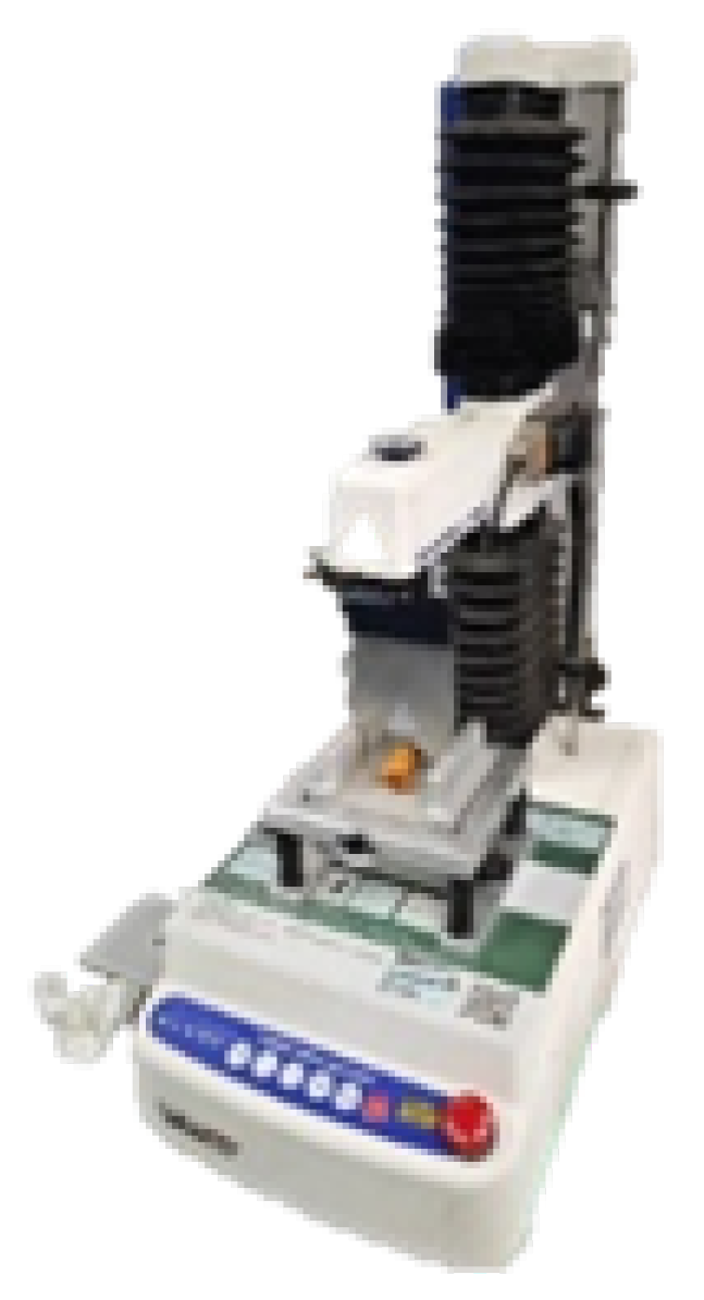
Shear modulus measurements were conducted using the TA.XT Plus texture analyzer from SMS (Figure 2), equipped with an HDP/WBV 60° V-shaped cutter for shear testing. The experimental data for the three materials are presented in Figure 3. Based on the data in Figure 3, the average shear moduli were calculated as follows: 1.19 MPa for diced chicken, 13.37 MPa for peanuts, and 7.88 MPa for diced scallions.

The relationship between the elastic modulus, Poisson’s ratio, and shear modulus is as follows:

$$S={\displaystyle \frac{E}{2(1+P)}}$$

(1)

where S is the shear modulus (MPa), E is the elastic modulus (MPa), and P is the Poisson’s ratio. P was taken as 0.450 for diced chicken, 0.362 for peanuts, and 0.360 for diced scallions. Based on this, the calculated elastic moduli were 3.45 MPa for diced chicken, 36.42 MPa for peanuts, and 21.43 MPa for diced scallions.

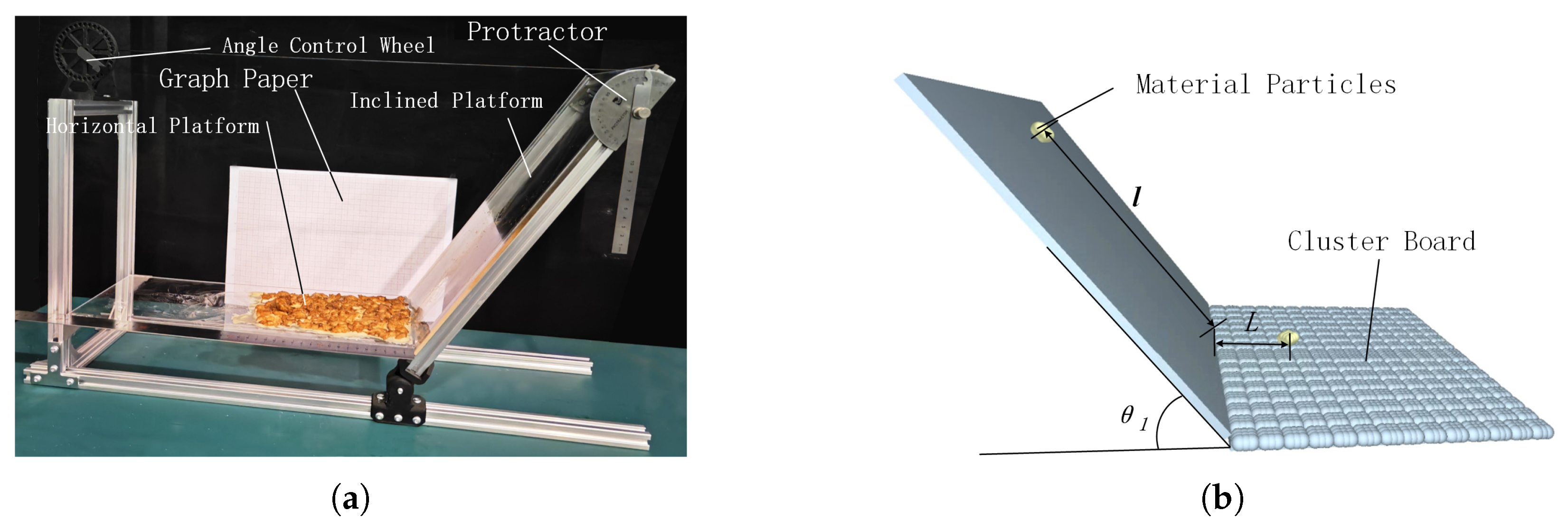
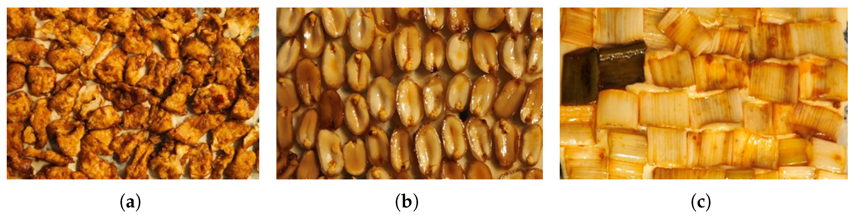
The static friction coefficient was determined using the inclined plane method [27]. The experimental setup is shown in Figure 4a, which consisted of an angle control wheel, protractor, inclined platform, and sheet of coordinate paper. The experiment involved placing the test surface on an inclined platform, positioning the material to be tested on the surface, and slowly adjusting the angle of inclination. A high-frame-rate camera was used to record the motion of the material, and the angle of the surface at which the material began to slide was measured. The experiment used diced chicken, peanuts, and diced scallions as the test materials, with PMMA, diced chicken cluster boards, peanut cluster boards, and diced scallion cluster boards as the test surfaces, as shown in Figure 5.

The experiment was conducted on the inclined plane testing platform shown in Figure 4a, with a total of 12 sets of measurements, and 20 measurements per set. The static friction coefficient was calculated using the following equations, and the average value was taken from the results:

$$\left.\begin{array}{c}{F}_1=Gsin\theta \\ F_2=Gcos\theta \\ F_1-f=0\\ F_2-N=0\\ f=\mu F_2\end{array}\right\}$$

(2)

where $F_1$ is the reaction force of the friction between the test material and the test surface (N), $F_2$ is the pressure exerted by the test material on the test surface (N), G is the gravitational force acting on the test material (N), f is the frictional force between the test material and the test surface (N), N is the supporting force exerted by the test surface on the test material (N), $\mu$ is the coefficient of friction between the test surface and the test material, and $\theta$ is the critical angle at which sliding occurred.

In the EDEM static friction test shown in Figure 4b, all the contact coefficients except for static friction were set to 0. The accurate sliding angle ($\theta$) was used as the independent variable, and the static friction coefficient was the test variable. The range of the static friction coefficient was set between 0.1 and 0.5, with an interval of 0.05. A total of 12 sets of simulation tests were performed, with each set repeated 10 times, and the average value was taken. Data fitting was used to determine the relationship between the static friction coefficient ($\mu$) and the critical sliding angle ($\theta$).

3.2.1. Poly(methyl methacrylate) (PMMA) Board Experiment and Simulation Results

The average sliding friction angles for the three different test materials were as follows: 18.6° for diced chicken, 25.8° for peanuts, and 46.1° for diced scallions. The corresponding average static friction coefficients between the three materials and the PMMA board were as follows: 0.337 for diced chicken, 0.483 for peanuts, and 1.039 for diced scallions.

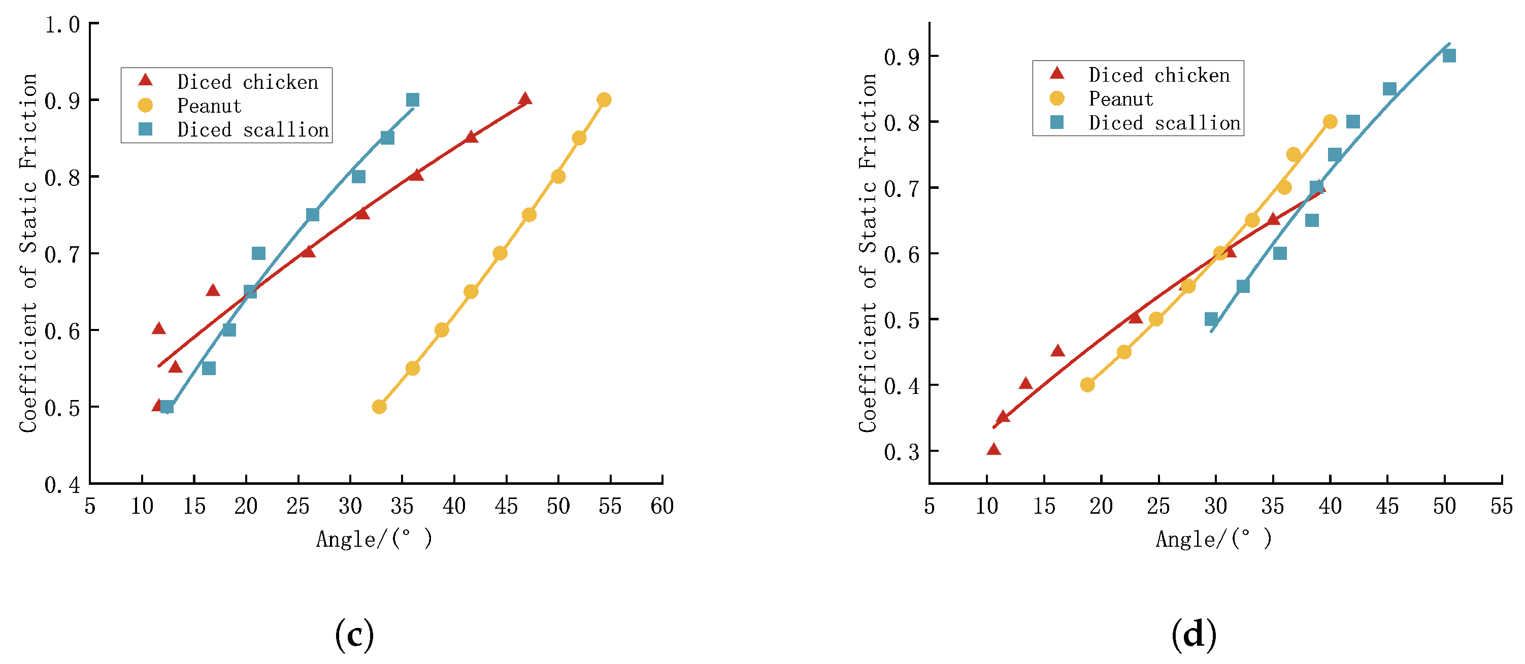
In the EDEM simulation experiments, the following fitted equations for diced chicken, peanuts, and diced scallions were, respectively, obtained, with the corresponding fitting curves displayed in Figure 6a:

$$\begin{array}{c}\mu =0.011+0.014\theta +1.1\times {10}^{-4}{\theta }^2,\left(\mathrm{diced}\mathrm{chicken}\right)\\ \mu =0.019+0.014\theta +{10}^{-4}{\theta }^2,\left(\mathrm{peanuts}\right)\\ \mu =-0.023+0.013\theta +{10}^{-4}{\theta }^2,\left(\mathrm{diced}\mathrm{scallions}\right)\end{array}$$

(3)

When the sliding friction angles were set to 18.6° for diced chicken, 25.8° for peanuts, and 46.1° for diced scallions, the friction coefficients between the test materials and the PMMA board were calculated as 0.308 for diced chicken, 0.448 for peanuts, and 0.789 for diced scallions.

3.2.2. Diced Chicken Cluster Board Experiment and Simulation Results

The average sliding friction angles for the three different test materials were as follows: 51.0° for diced chicken, 34.0° for peanuts, and 38.8° for diced scallions. The corresponding average static friction coefficients between the three materials and the diced chicken cluster board were 1.234 for diced chicken, 0.675 for peanuts, and 0.804 for diced scallions.

In the EDEM simulation experiments, the following fitted equations for diced chicken, peanuts, and diced scallions were, respectively, obtained with the corresponding fitting curves displayed in Figure 6b:

$$\begin{array}{c}\mu =-0.065+0.02\theta -7.896\times {10}^{-5}{\theta }^2,\left(\mathrm{diced}\mathrm{chicken}\right)\\ \mu =-0.375+0.03\theta -2.953\times {10}^{-4}{\theta }^2,\left(\mathrm{peanuts}\right)\\ \mu =0.339+0.012\theta -1.563\times {10}^{-5}{\theta }^2,\left(\mathrm{diced}\mathrm{scallions}\right)\end{array}$$

(4)

When the sliding friction angles were set to 51.0° for diced chicken, 34.0° for peanuts, and 38.8° for diced scallions, the friction coefficients between the test materials and the diced chicken cluster board were calculated as 0.758 for diced chicken, 0.667 for peanuts, and 0.768 for diced scallions.

3.2.3. Peanut Cluster Board Experiment and Simulation Results

The average sliding friction angles for the three different test materials were as follows: 41.6° for diced chicken, 43° for peanuts, and 41.8° for diced scallions. The corresponding average static friction coefficients for the three materials were 0.888 for diced chicken, 0.933 for peanuts, and 0.894 for diced scallions.

In the EDEM simulation experiments, the following fitted equations for diced chicken, peanuts, and diced scallions were, respectively, obtained with the corresponding fitting curves presented in Figure 6c:

$$\begin{array}{c}\mu =0.417+0.012\theta -4.288\times {10}^{-5}{\theta }^2,\left(\mathrm{diced}\mathrm{chicken}\right)\\ \mu =0.138+0.007\theta +1.35\times {10}^{-4}{\theta }^2,\left(\mathrm{peanuts}\right)\\ \mu =0.206+0.025\theta -1.755\times {10}^{-4}{\theta }^2,\left(\mathrm{diced}\mathrm{scallions}\right)\end{array}$$

(5)

When the sliding friction angles were set to 41.6° for diced chicken, 43° for peanuts, and 41.8° for diced scallions, the friction coefficients between the test materials and the peanut cluster board were calculated as 0.851 for diced chicken, 0.673 for peanuts, and 0.944 for diced scallions.

3.2.4. Diced Scallion Cluster Board Experiment and Simulation Results

The average sliding friction angles for the three different test materials were as follows: 30.6° for diced chicken, 36.6° for peanuts, and 44.2° for diced scallions. The corresponding average static friction coefficients for the three materials were 0.591 for diced chicken, 0.743 for peanuts, and 0.972 for diced scallions.

In the EDEM simulation experiments, the following fitted equations for diced chicken, peanuts, and diced scallions were, respectively, obtained with the corresponding fitting curves displayed in Figure 6d:

$$\begin{array}{c}\mu =0.165+0.017\theta -9.322\times {10}^{-5}{\theta }^2,\left(\mathrm{diced}\mathrm{chicken}\right)\\ \mu =0.182+0.008\theta +1.833\times {10}^{-4}{\theta }^2,\left(\mathrm{peanuts}\right)\\ \mu =-0.496+0.04\theta -2.379\times {10}^{-4}{\theta }^2,\left(\mathrm{diced}\mathrm{scallions}\right)\end{array}$$

(6)

When the sliding friction angles were set to 30.6° for diced chicken, 36.6° for peanuts, and 44.2° for diced scallions, the friction coefficients between the test materials and the diced scallion cluster board were calculated as 0.602 for diced chicken, 0.727 for peanuts, and 0.809 for diced scallions.

3.2.5. Static Friction Coefficient Calibration Conclusions

The results of the experimental and simulation calibration showed that the static friction coefficients between the PMMA board and the diced chicken, peanuts, and diced scallions were 0.308, 0.448, and 0.789, respectively. The static friction coefficients between the diced chicken, peanuts, and diced scallions were as follows: 0.758 for diced chicken, 0.673 for peanuts, and 0.809 for diced scallions.

Two friction coefficient values were measured for each material pair, and the results are shown in

Table 2. Relative errors between simulation and experimental values of static friction coefficient for different materials.

Material Pair	Simulation Value	Experimental Value	Relative Error
Diced chicken–Peanut cluster board	0.851	0.888	4.61%
Peanut–Diced chicken cluster board	0.667	0.675	1.19% *
Diced chicken–Diced scallion cluster board	0.602	0.589	1.86% *
Diced scallion–Diced chicken cluster board	0.768	0.735	4.78%
Peanut–Diced scallion cluster board	0.727	0.742	2.15% *
Diced scallion–Peanut cluster board	0.944	0.894	5.59%

Note: The asterisk (*) indicates that the simulation results for this parameter had a small error compared to the experimental values.

. The pairs with smaller relative errors are indicated with an asterisk. The static friction coefficients with the minimum errors compared to the actual experimental measurements were selected and are shown as follows:

• Diced chicken–Peanuts: 0.667
• Diced chicken–Diced scallions: 0.602
• Peanuts–Diced scallions: 0.727

3.3. Rolling Friction Coefficient

The rolling friction coefficient was determined using the rolling distance method [28]. The experimental setup shown in Figure 7 consisted of an angle control wheel, protractor, flat platform, inclined platform, and sheet of coordinate paper. The experiment involved placing the test surface on the flat platform, positioning the material to be tested on the inclined platform at a specified angle and distance, and recording the rolling process and distance of the material using a high-frame-rate camera. The rolling friction coefficient between the material and the surface was then calculated. Diced chicken, peanuts, and diced scallions were used as test materials, while PMMA, diced chicken cluster boards, peanut cluster boards, and diced scallion cluster boards were used as test surfaces.

After multiple preliminary experiments, the actual experimental parameters were set to ${\theta }_1$ = 60° and l = 200 mm. A total of 12 sets of measurements were conducted, with 20 measurements per set. The rolling friction coefficient was calculated using the following equation, and the average value was taken:

$$Glsin{\theta }_1=G(lcos{\theta }_1+L)\times (\delta +\mu )$$

(7)

where G is the gravitational force on the test material (N), l is the linear distance from the test material to the base of the inclined plane (mm), ${\theta }_1$ is the angle between the inclined plane and the horizontal surface (°), L is the rolling distance of the test material on the flat surface (mm), and $\delta$ is the rolling friction coefficient of the test material.

The EDEM rolling friction test, as shown in Figure 7b, involved setting all the contact coefficients to 0 except for the rolling friction coefficient and the static friction coefficient. The sliding distance L on the plane was used as the test indicator, with the rolling friction coefficient as the test variable. The rolling friction coefficient ranged from 0.02 to 0.40, with an interval of 0.02, and 10 points were taken for each set. A total of 12 simulation tests were performed, each repeated 10 times, and the average value was calculated. Data fitting was used to determine the relationship between the static friction coefficient $\delta$ and the sliding distance L.

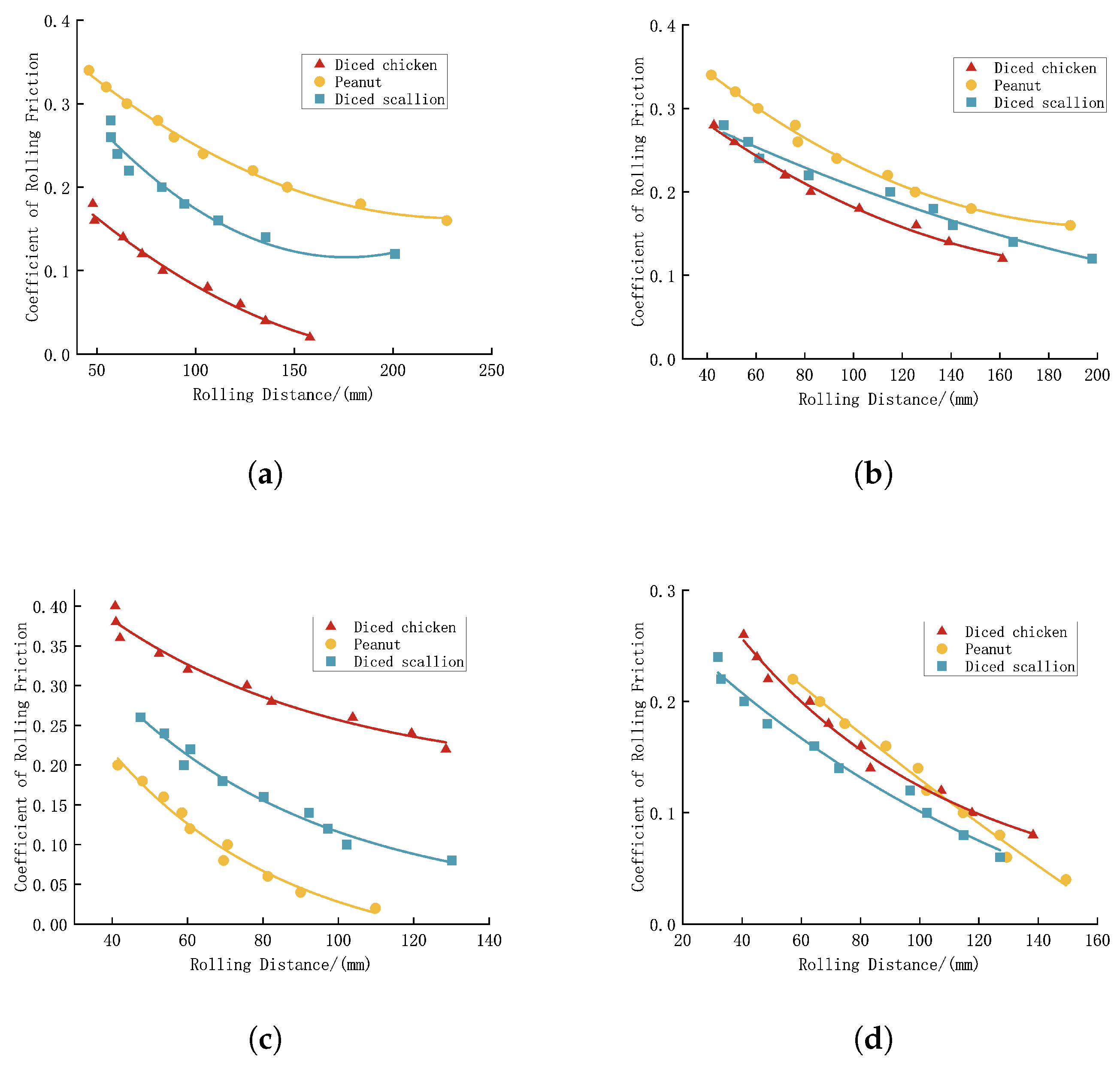
3.3.1. PMMA Board Experiment and Simulation Results

The average rolling distances for the three different test materials were as follows: 135.3 mm for diced chicken, 121.1 mm for peanuts, and 104 mm for diced scallions. The corresponding average static friction coefficients between the three materials and the PMMA board were 0.045 for diced chicken, 0.227 for peanuts, and 0.163 for diced scallions.

In the EDEM simulation experiments, the following fitted equations for diced chicken, peanuts, and diced scallions were, respectively, obtained, with the corresponding fitting curves presented in Figure 8a:

$$\begin{array}{c}\delta =-0.03457-0.3738\times 0.{98832}^L(R_2=0.98571),\left(\mathrm{diced}\mathrm{chicken}\right)\\ \delta =0.13106-0.34167\times 0.{98931}^L(R_2=0.99845),\left(\mathrm{peanuts}\right)\\ \delta =0.12532-0.74818\times 0.{97076}^L(R_2=0.97414),\left(\mathrm{diced}\mathrm{scallions}\right)\end{array}$$

(8)

When the sliding distances were set to 135.3 mm for diced chicken, 121.1 mm for peanuts, and 104 mm for diced scallions, the friction coefficients between the test materials and the PMMA board were calculated as 0.042 for diced chicken, 0.224 for peanuts, and 0.159 for diced scallions.

3.3.2. Diced Chicken Cluster Board Experiment and Simulation Results

The average rolling distances for the three different test materials were as follows: 88.5 mm for diced chicken, 98.5 mm for peanuts, and 111.3 mm for diced scallions. The corresponding average static friction coefficients between the three materials and the diced chicken cluster board were 0.161 for diced chicken, 0.247 for peanuts, and 0.189 for diced scallions.

In the EDEM simulation experiments, the following fitted equations for the diced chicken, peanuts, and diced scallions were, respectively, derived with the corresponding fitting curves presented in Figure 8b:

$$\begin{array}{c}\delta =0.0563-0.34076\times 0.{99}^L(R_2=0.9956),\left(\mathrm{diced}\mathrm{chicken}\right)\\ \delta =0.11231-0.36523\times 0.{989}^L(R_2=0.99288),\left(\mathrm{peanuts}\right)\\ \delta =-0.02869-0.37319\times 0.{99536}^L(R_2=0.98063),\left(\mathrm{diced}\mathrm{scallions}\right)\end{array}$$

(9)

When the sliding distances were set to 88.5 mm for diced chicken, 98.5 mm for peanuts, and 111.3 mm for diced scallions, the friction coefficients between the test materials and the diced chicken cluster board were calculated as 0.196 for diced chicken, 0.235 for peanuts, and 0.191 for diced scallions.

3.3.3. Peanut Cluster Board Experiment and Simulation Results

The average rolling distances for the three different test materials were as follows: 92 mm for diced chicken, 94 mm for peanuts, and 122.5 mm for diced scallions. The corresponding average static friction coefficients between the three materials and the peanut cluster board were 0.251 for diced chicken, 0.154 for peanuts, and 0.083 for diced scallions.

In the EDEM simulation experiments, the following fitted equations for diced chicken, peanuts, and diced scallions were, respectively, derived with the corresponding fitting curves presented in Figure 8c:

$$\begin{array}{c}\delta =-0.03457-0.3738\times 0.{98832}^L(R_2=0.98571),\left(\mathrm{diced}\mathrm{chicken}\right)\\ \delta =0.13106-0.34167\times 0.{98931}^L(R_2=0.99845),\left(\mathrm{peanuts}\right)\\ \delta =0.12532-0.74818\times 0.{97076}^L(R_2=0.97414),\left(\mathrm{diced}\mathrm{scallions}\right)\end{array}$$

(10)

When the sliding distances were set to 92 mm for diced chicken, 94 mm for peanuts, and 122.5 mm for diced scallions, the friction coefficients between the test materials and the peanut cluster board were calculated as follows: 0.262 for diced chicken, 0.146 for peanuts, and 0.085 for diced scallions.

3.3.4. Diced Scallion Cluster Board Experiment and Simulation Results

The average rolling distances for the three different test materials were as follows: 88.5 mm for diced chicken, 112.5 mm for peanuts, and 111.7 mm for diced scallions. The corresponding average static friction coefficients between the three materials and the diced scallion cluster board were as follows: 0.137 for diced chicken, 0.096 for peanuts, and 0.071 for diced scallions.

In the EDEM simulation experiments, the following fitted equations for the diced chicken, peanuts, and diced scallions were, respectively, obtained with the corresponding fitting curves presented in Figure 8d:

$$\begin{array}{c}\delta =0.01874-0.40977\times 0.{98648}^L(R_2=0.98967),\left(\mathrm{diced}\mathrm{chicken}\right)\\ \delta =-0.90331-1.2574\times 0.{99804}^L(R_2=0.98954),\left(\mathrm{peanuts}\right)\\ \delta =-0.09559-0.40454\times 0.{99283}^L(R_2=0.98172),\left(\mathrm{diced}\mathrm{scallions}\right)\end{array}$$

(11)

When the sliding distances were set to 88.5 mm for diced chicken, 112.5 mm for peanuts, and 111.7 mm for diced scallions, the friction coefficients between the test materials and the diced scallion cluster board were calculated as 0.141 for diced chicken, 0.103 for peanuts, and 0.085 for diced scallions.

3.3.5. Rolling Friction Coefficient Calibration Conclusions

The results of the experimental and simulation calibration showed that the dynamic friction coefficients between the PMMA board and the diced chicken, peanuts, and diced scallions were 0.042, 0.224, and 0.159, respectively. The dynamic friction coefficients between the diced chicken, peanuts, and diced scallions were 0.196 for diced chicken, 0.146 for peanuts, and 0.085 for diced scallions.

Two friction coefficient values were measured for each material pair, and the results are summarized in

Table 3. Relative Errors between Simulation and Experimental Values of Rolling Friction Coefficient for Different Materials.

Material Pair	Simulation Value	Experimental Value	Relative Error
Diced chicken–Peanut cluster board	0.262	0.251	5.99%
Peanut–Diced chicken cluster board	0.235	0.247	4.86% *
Diced chicken–Diced scallion cluster board	0.141	0.137	2.84%
Diced scallion–Diced chicken cluster board	0.191	0.189	1.05% *
Peanut–Diced scallion cluster board	0.103	0.096	6.80%
Diced scallion–Peanut cluster board	0.085	0.083	2.35% *

Note: The asterisk (*) indicates that the simulation results for this parameter had a small error compared with the experimental values.

. Pairs with smaller relative errors are marked with an asterisk. The static friction coefficients selected, based on the minimal error compared with the actual experimental measurements, were as follows:

• Diced chicken–Peanuts: 0.247
• Diced chicken–Diced scallions: 0.189
• Peanuts–Diced scallions: 0.083

3.4. Coefficient of Restitution

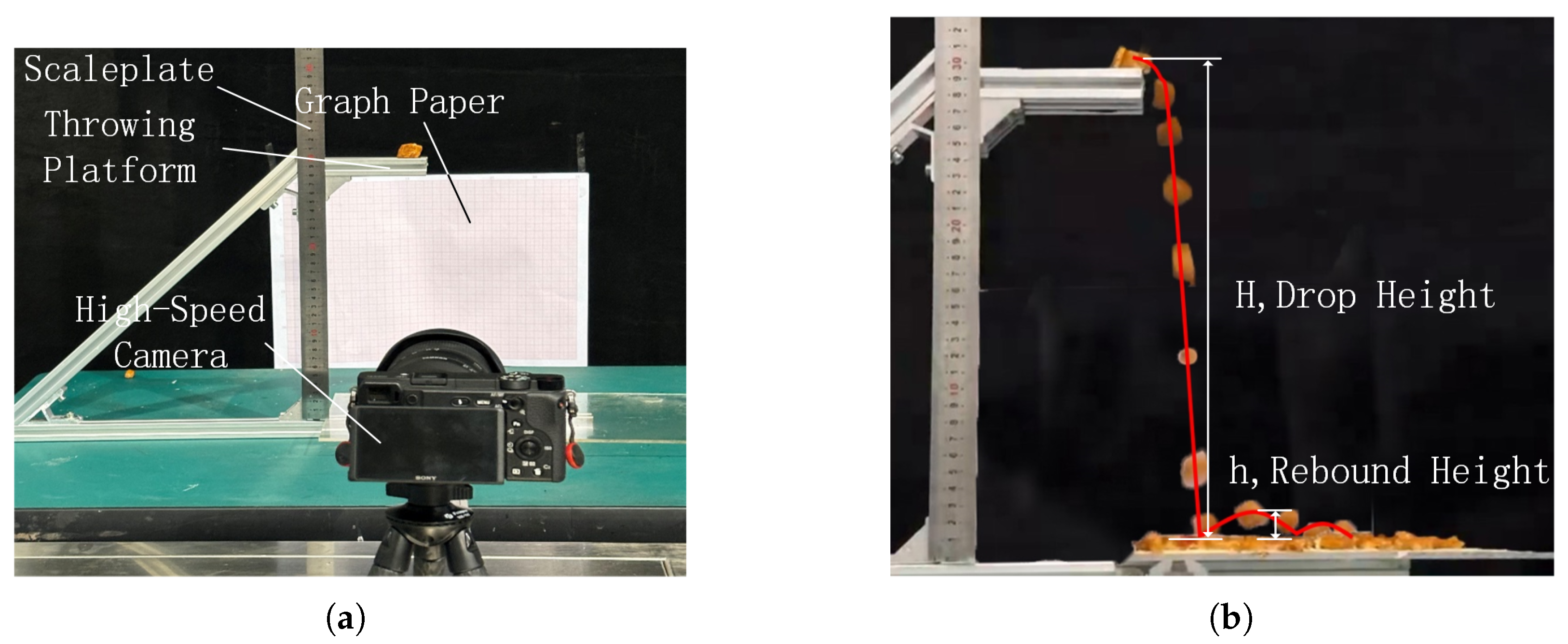
The coefficient of restitution was determined using the rebound height method [29,30]. The experimental setup, as shown in Figure 9, consisted of a support stand, drop platform, flat platform, sheet of coordinate paper, and high-speed camera. The experiment involved placing the test surface on the flat platform, positioning the test material on the drop platform, and recording the drop process using a high-frame-rate camera. The coefficient of restitution between the material and the test surface was then calculated. Diced chicken, peanuts, and diced scallions were used as test materials, with PMMA, diced chicken cluster boards, peanut cluster boards, and diced scallion cluster boards used as the test surfaces.

After multiple preliminary experiments, the drop height was set to H = 300 mm. A total of 12 sets of measurements were conducted, with 20 measurements per set. The coefficient of restitution was calculated as follows, and the average value was taken:

$$e={\displaystyle \frac{v_1}{v_2}}={\displaystyle \frac{\sqrt{2gh}}{\sqrt{2gH}}}={\displaystyle \frac{\sqrt{h}}{\sqrt{H}}}$$

(12)

where e is the coefficient of restitution, $v_1$ is the relative velocity during rebound (mm/s), $v_2$ is the relative velocity during impact (mm/s), g is the acceleration due to gravity (m/$s^2$), h is the maximum rebound height (mm), and H is the drop height (mm).

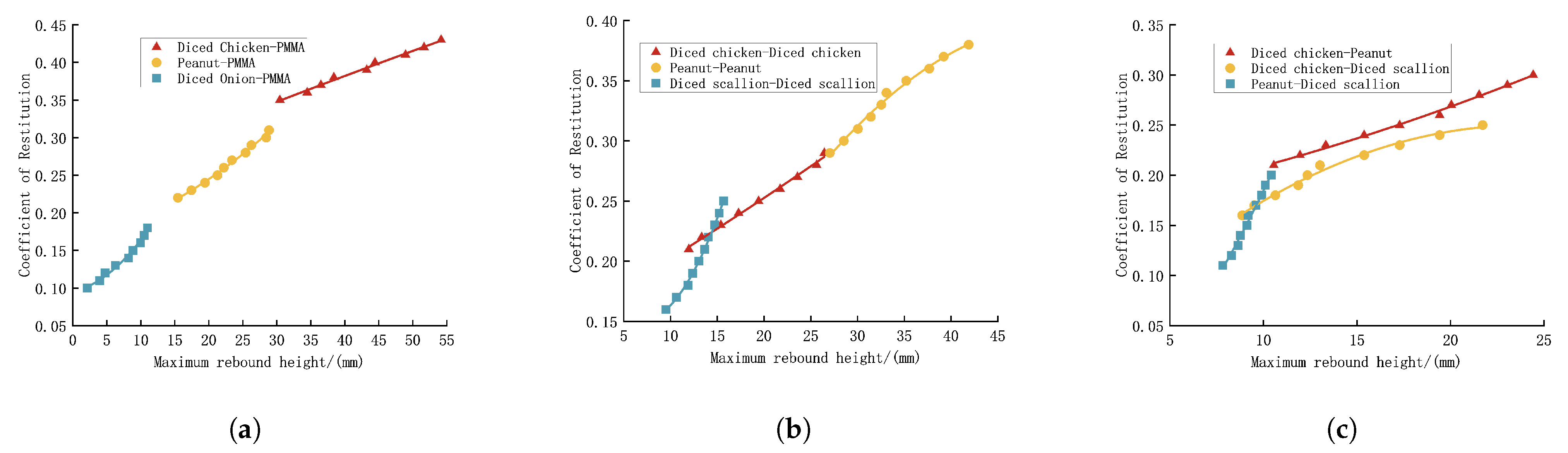
In the EDEM rebound height tests, the rolling friction coefficients and static friction coefficients were set according to the calibration results from Section 3.3 and Section 3.4, respectively. The maximum rebound height h was used as the test indicator, with the coefficient of restitution as the test variable. Ten points were taken for each group. A total of nine simulation tests were performed, with each set repeated 10 times, and the average value was calculated. Data fitting was used to determine the relationship between the coefficient of restitution e and the maximum rebound height h. The fitting curves shown in Figure 10 corresponded to the following equations. The results are summarized in

Table 4. Simulation Fitting of Crash Recovery Coefficient for Different Materials.

Parameter	Maximum Rebound Height h/(mm)	Experimentally Measured e	Simulated (Fitted) e
Diced chicken–PMMA	50.5	0.41	0.417
Peanut–PMMA	21.2	0.266	0.252
Diced scallion–PMMA	5.1	0.13	0.118
Diced chicken–Diced chicken	17.6	0.242	0.24
Diced chicken–Peanut	20.7	0.263	0.273
Diced chicken–Diced scallion	13.2	0.21	0.205
Peanut–Peanut	34.8	0.341	0.345
Peanut–Diced scallion	8.2	0.165	0.12
Diced scallion–Diced scallion	13.2	0.21	0.202

.

$$\begin{array}{c}e=0.2385+0.0038h-5.0704\times {10}^{-6}{h}^2(R_2=0.99249),\\ (\mathrm{diced}\mathrm{chicken}-\mathrm{PMMA})\\ e=0.1645+0.0019h+1.0581\times {10}^{-4}{h}^2(R_2=0.99353),\\ (\mathrm{peanuts}-\mathrm{PMMA})\\ e=0.0953+0.002h+4.8049\times {10}^{-4}{h}^2(R_2=0.98666),\\ (\mathrm{diced}\mathrm{scallions}-\mathrm{PMMA})\\ e=0.1556+0.0045h+1.657\times {10}^{-5}{h}^2(R_2=0.99521),\\ (\mathrm{diced}\mathrm{chicken}-\mathrm{diced}\mathrm{chicken})\\ e=-0.0785+0.0183h-1.7472\times {10}^{-4}{h}^2(R_2=0.99304),\\ (\mathrm{peanuts}-\mathrm{peanuts})\\ e=0.2044-0.0165h+1.24\times {10}^{-3}{h}^2(R_2=0.9975),\\ (\mathrm{diced}\mathrm{scallions}-\mathrm{diced}\mathrm{scallions})\\ e=0.1665+0.0035h+8.1946\times {10}^{-5}{h}^2(R_2=0.99541),\\ (\mathrm{diced}\mathrm{chicken}-\mathrm{peanuts})\\ e=0.2385+0.0038h-5.0704\times {10}^{-6}{h}^2(R_2=0.99249),\\ (\mathrm{diced}\mathrm{chicken}-\mathrm{diced}\mathrm{scallions})\\ e=-0.0512+0.0084h+1.52\times {10}^{-3}{h}^2(R_2=0.99052),\\ (\mathrm{peanuts}-\mathrm{diced}\mathrm{scallions})\end{array}$$

(13)

4. Contact Parameter Calibration

4.1. Angle of Repose Experiment and Simulation

The angle of repose refers to the maximum angle between the surface of a piled material and the horizontal plane at which the material remains stable without sliding. It is a key parameter reflecting the flowability, cohesion, and frictional properties of particulate or discrete materials, and is, therefore, commonly used as a benchmark for validating DEM simulation parameters. The static angles of repose of the primary materials and their mixture in Kung Pao Chicken on PMMA were measured using the funnel method [30]. Each material was measured 10 times, and images of the stable pile were captured using a camera on the stacking surface. After contour extraction in Photoshop (PS), the edge contour points were digitized, and the coordinates were extracted using the Digitizer software. Finally, the scatter points were linearly fitted using the Origin software to obtain the angles of repose on both sides. The actual process of measuring the angle of repose is shown in Figure 11.

From the experiments, the measured angles of repose on the PMMA surface were determined to be as follows:

• Kung Pao Chicken mixture: 29.96°
• Diced chicken: 32.99°
• Peanuts: 27.99°
• Diced scallions: 35.89°

A funnel was modeled in SolidWorks 2020 SP5.0, with the funnel material being 304 stainless steel. The EDEM simulation configuration was consistent with the experimental setup, as shown in Figure 12. The funnel lifting speed was set to 20 mm/s, and the total mass of the materials was 250 g. The contact energies between the different materials were approximately within 2 J/m², with different contact energies tested at intervals of 0.2 J/m².

The simulation results are shown in Figure 12. By substituting the actual angles of repose into the fitted equations, the following surface energy values for the material pairs were obtained.

• Diced chicken–Diced chicken: 0.88 J/m²
• Peanuts–Peanuts: 0.39 J/m²
• Diced scallions–Diced scallions: 1.66 J/m²

4.2. Steepest Slope Experiment

The steepest slope experiment was designed to find the optimal ranges for the remaining contact energy parameters.

• $X_1$ represents the contact energy for diced chicken and peanuts, with a range of 0.2 to 1.0 J/m².
• $X_2$ represents the contact energy for diced chicken and diced scallions, with a range of 0.6 to 1.8 J/m².
• $X_3$ represents the contact energy for peanuts and diced scallions, with a range of 0.2 to 1.8 J/m².

The optimal values for these contact energy parameters were determined by simulating the angle of repose for the mixture. The relative error between the simulated and experimental angles of repose was used to evaluate the simulation results. A steepest slope experiment was designed to systematically determine the optimal contact energy values, and the results are shown in

Table 5. Design and results of steepest climb test scheme.

No.	Factor			Evaluation
	X1 (J/m2)	X2 (J/m2)	X3 (J/m2)	Angle of Repose (°)	Relative Error (%)
1	0.20	0.60	0.20	25.71	14.19%
2	0.40	0.90	0.40	28.07	6.31%
3	0.60	1.20	0.60	30.82	1.07%
4	0.80	1.50	1.40	33.89	13.11%
5	1.00	1.80	1.80	35.45	18.42%

.

4.3. Box–Behnken Experimental Design

Upon analyzing the data in Table 5, it was observed that the relative error in the third measurement was the smallest. Therefore, the optimal range was determined to be between the third group and the second and fourth groups. The experimental factor levels are shown in

Table 6. Box–Behnken design (BBD) test factor level coding table.

Coding	Factor
	X1 (J/m2)	X2 (J/m2)	X3 (J/m2)
−1	0.40	0.90	0.60
0	0.60	1.20	1.00
1	0.80	1.50	1.40

, and the experimental design and results are presented in

Table 7. Box–Behnken design (BBD) experimental design and results.

Test No.	Factor			Evaluation
	X1 (J/m2)	X2 (J/m2)	X3 (J/m2)	Angle of Repose (°)	Relative Error (%)
1	1	1	0	30.96	3.35
2	0	0	0	29.36	2.01
3	−1	−1	0	33.21	10.85
4	0	0	0	30.23	0.90
5	0	0	0	29.35	2.02
6	0	−1	−1	33.10	10.47
7	0	0	0	29.92	0.13
8	0	0	0	30.17	0.71
9	−1	0	−1	34.43	14.90
10	1	−1	0	31.68	05.74
11	0	−1	1	30.19	0.77
12	0	1	−1	32.16	7.33
13	−1	1	0	34.11	13.85
14	0	1	1	31.25	4.31
15	1	0	1	30.27	1.04
16	1	0	−1	31.04	3.61
17	−1	0	1	31.64	5.60

.

4.3.1. Regression Model Analysis

Through multiple regression fitting analysis of the experimental results, a second-order regression model was obtained to relate the angle of repose of the Kung Pao Chicken mixture to the three significant parameters. The regression equation is as follows:

$$\begin{array}{c}Y=31.2599-1.3172X_1-0.8968X_2-0.5204X_3-0.2247X_1{X}_2+0.2108X_1{X}_3+0.1392X_2{X}_3\\ +0.9829X_1^2+0.3736X_2^2+0.075X_3^2\end{array}$$

(14)

The analysis of variance results of the regression model are shown in

Table 8. Analysis of variance of the regression model.

Source of Variation	Mean Square	Degrees of Freedom	Sum of Squares	F-Statistic	p-Value
Model	0.0359	9	0.0040	96.31	<0.0001 **
$X_1$	0.0124	1	0.0124	298.62	<0.0001 **
$X_2$	0.0000	1	0.0000	0.3082	0.5961
$X_3$	0.0076	1	0.0076	182.56	<0.0001 **
$X_1{X}_2$	0.0007	1	0.0007	17.56	0.0041 *
$X_1{X}_3$	0.0011	1	0.0011	27.46	0.0012 *
$X_2{X}_3$	0.0011	1	0.0011	26.94	0.0013 *
$X_1^2$	0.0065	1	0.0065	157.13	<0.0001 **
$X_2^2$	0.0048	1	0.0048	114.93	<0.0001 **
$X_3^2$	0.0006	1	0.0006	14.64	0.0065 *
Residual	0.0003	7	0.0000
Lack of Fit	0.0000	3	3.44 × 10−6	0.0492	0.9836
Pure Error	0.0003	4	0.0001
Total	0.0362	16

Note: ** indicates a highly significant difference (p < 0.001), * indicates a significant difference (p < 0.05).

. The regression model was highly significant (p < 0.0001), with a good degree of fit for the regression equation ($R^2$ = 0.9920). The adjusted coefficient of determination was $R_{adj}^2$ = 0.9817, indicating a good correlation of the fit. The predicted coefficient of determination was $R_{pre}^2$ = 0.9834, with the difference from the adjusted coefficient being less than 0.2, confirming that the model was valid. The interaction terms all had a significant impact on the results. The coefficient of variation for the model was 12.49%, suggesting that the experiment was generally reliable. The accuracy was 28.63%, indicating a high level of precision.

The relative error showed a trend of first decreasing and then increasing, with the trend being insignificant when the contact energy between the diced chicken and diced scallions ($X_2$) was at an intermediate value. The shape of the response surface was concave in the middle, indicating a strong interaction between the contact energies of the diced chicken and peanuts ($X_1$) and the diced chicken and diced scallions ($X_2$).

From Figure 13b, it can be seen that when the contact energy between the peanuts and diced scallions ($X_3$) was small, the relative error decreased as the contact energy between the diced chicken and peanuts ($X_1$) increased. The response surface was steep, with a large gradient.

According to Figure 13c, the response surface also exhibited a concave shape in the middle, but it was relatively smooth with a small slope and minimal curvature. The contour lines were almost parallel, indicating that the interactions between the diced chicken–diced scallions contact energy ($X_2$) and peanuts–diced scallions contact energy ($X_3$) had the lowest effect on the relative error of the angle of repose.

4.3.2. Parameter Optimization and Model Validation

Based on the second-order regression model, multi-objective optimization was performed to find the optimal parameter values, resulting in five usable sets of data. Simulations were conducted with these five sets, and the simulation results and corresponding relative errors are presented in

Table 9. Optimization results and simulation results.

No.	Factor			Evaluation
	X1 (J/m2)	X2 (J/m2)	X3 (J/m2)	Angle of Repose (°)	Relative Error (%)
1	0.653	1.1	1.107	29.98	0.05
2	0.685	1.265	1.296	30.00	0.13
3	0.644	1.16	1.089	29.89	0.24
4	0.64	1.286	1.257	30.15	0.62
5	0.671	1.262	1.101	30.17	0.71

.

The DEM simulation for the angle of repose of the Kung Pao Chicken mixture is shown in Figure 14. Simulations with each set of data were repeated 10 times, and the average value was taken. The final simulation resulted in the smallest relative error of 0.05% compared with the actual measured angle of repose. These results demonstrated that the contact parameters of the Kung Pao Chicken mixture calibrated using this model were reliable.

5. Discussion

This study proposes a parameter calibration method for DEM simulation of viscous, multi-component food materials, using Kung Pao Chicken as a representative case. The method addresses a key challenge in simulation-driven equipment design—namely, the lack of accurate material parameters for complex food systems.

While the findings are based on a single dish, Kung Pao Chicken reflects typical characteristics of many Chinese cooked dishes, including discrete solid components and adhesive sauces. The proposed method is extendable and will be tested on a broader range of dishes in future work. We also plan to investigate the adaptability of food-filling equipment across different dish types.

It is important to note that the physical properties of food materials can be significantly affected by various internal components, such as oil, starch, and fiber, as well as by processing conditions including temperature, moisture content, and cooking methods. These factors can influence inter-particle adhesion, flowability, and deformation behavior during handling and portioning. However, the focus of this study is to evaluate the accuracy of a parameter calibration method for viscous and multi-component food materials, rather than to systematically investigate the effects of each influencing factor. Nevertheless, further exploration of how these variables affect material properties remains a valuable direction for future research, particularly in the context of developing more robust and generalizable DEM models for food applications [31].

The experimental validation of the calibrated parameters has been carried out by comparing the simulated and actual angles of repose, demonstrating the accuracy and reliability of the DEM model. While the development of a physical prototype was beyond the scope of this study, future validation using a real portioning system would further strengthen the connection between simulation and practical application. This study provides a foundation for simulation-driven design in food equipment engineering and contributes to the advancement of intelligent kitchen automation.

6. Conclusions

1.

The DEM parameter calibration for the viscous Kung Pao Chicken dish using the JKR contact model was validated through simulation–experiment comparison. The static and dynamic friction coefficients were determined via quadratic fitting, while the coefficient of restitution was calibrated using exponential fitting. All the fitting results demonstrated strong agreement, with the lowest coefficient of determination being $R^2$ = 0.9741.

2.

For the JKR parameters of material pairs that could not be directly measured, a second-order regression model was constructed to relate the contact energy parameters to the relative error of the angle of repose, based on the steepest slope and Box–Behnken experiments. By using a multi-objective optimization algorithm, the optimal combinations were determined, resulting in the following optimal contact energy values.

• Diced chicken–Peanuts: 0.653 J/m²
• Diced chicken–Diced scallions: 1.1 J/m²
• Peanuts–Diced scallions: 1.107 J/m²

3.

The study demonstrates the feasibility of constructing accurate DEM models for viscous, multi-component Chinese dishes by combining physical experiments with stepwise simulation fitting. The final model showed excellent agreement with physical tests, with a relative error of only 0.05% in the angle of repose, confirming the reliability of the proposed calibration method.