Abstract
Photovoltaic panels are pivotal in transforming solar irradiance into electricity, making them a key technology in renewable energy. Despite their potential, the distribution of photovoltaic systems in Romania remains sparse, requiring advanced data analytics for effective management, particularly in addressing the intermittent nature of photovoltaic energy. This study investigates the predictive capabilities of Long Short-Term Memory (LSTM) and Convolutional Neural Network (CNN) architectures for forecasting hourly photovoltaic energy production in Romania. The results indicate that CNN models significantly outperform LSTM models, with 77% of CNNs achieving an R2 of 0.9 or higher compared to only 13% for LSTMs. The best-performing CNN model reached an R2 of 0.9913 with a mean absolute error (MAE) of 9.74, while the top LSTM model achieved an R2 of 0.9880 and an MAE of 12.57. The rapid convergence of the CNN model to stable error rates illustrates its superior generalization capabilities. Moreover, the model’s ability to accurately predict photovoltaic production over a two-day timeframe, which is not included in the testing dataset, confirms its robustness. This research highlights the critical role of accurate energy forecasting in optimizing the integration of photovoltaic energy into Romania’s power grid, thereby supporting sustainable energy management strategies in line with the European Union’s climate goals. Through this methodology, we aim to enhance the operational safety and efficiency of photovoltaic systems, facilitating their large-scale adoption and ultimately contributing to the fight against climate change.
1. Introduction
Photovoltaic (PV) technology, which converts solar irradiance into electrical energy, is now one of the most widely adopted renewable energy solutions worldwide [1]. Its growing role in the global energy mix is largely attributed to the urgent need for decarbonization, energy diversification, and a reduction in dependence on fossil fuels [2]. Among renewable technologies, PV systems offer distinct advantages due to their modularity, flexibility in deployment, and decentralization capabilities, making them particularly attractive in both urban and rural settings [3]. However, a major limitation of PV systems remains their intermittent and weather-dependent nature. PV energy production is highly variable, being influenced by external factors such as cloud cover, ambient temperature, solar irradiance, and seasonal cycles [4]. These fluctuations present significant challenges when integrating PV-generated electricity into the power grid, which is designed to operate based on predictable and continuous energy inputs [5,6].
The variability and uncertainty of PV output can lead to mismatches between supply and demand, especially during peak hours or periods of low irradiance. As PV penetration in the energy mix increases, these imbalances may jeopardize the stability and reliability of the power grid. Consequently, accurate short-term forecasting of PV energy production has become a critical research focus. Such predictions allow grid operators to plan resource allocation more effectively, minimize balancing costs, and maintain system reliability while maximizing the use of clean energy [7]. Moreover, reliable forecasting supports market participation, improves scheduling of ancillary services, and enables the integration of storage solutions or complementary renewable sources.
Recent progress in artificial intelligence (AI) and machine learning (ML) has opened new opportunities for modeling and forecasting PV output. In particular, neural network architectures such as Multilayer Perceptrons (MLPs), Long Short-Term Memory networks (LSTM), Convolutional Neural Networks (CNNs), and hybrid approaches have proven capable of capturing the complex, nonlinear relationships between environmental parameters and energy production [8,9]. For instance, refs. [10,11] enhance forecast accuracy using entity embedding within MLPs and integrate weather forecasts to improve two-day prediction windows across 16 PV plants in Northern Italy. In [12], an RBNN model supported by reinforcement learning and feature optimization demonstrates strong performance across PV systems ranging from 1 to 1000 units, using a wide array of evaluation metrics. Similarly, ref. [13] applies neural networks to rooftop PV systems, incorporating granular 15-min interval data and over thirty input features, including AC/DC electrical parameters and meteorological variables.
Beyond traditional models, various studies introduce hybrid architectures to tackle challenges like non-stationarity and limited data availability. For example, [14] combines empirical lab tests with field measurements for off-grid systems in Kuwait, while [15] compares CNNs and LSTM in ultra-short-term solar irradiance prediction, showing CNN superiority in most scenarios. Other contributions include transfer learning applied to PV generation forecasting when historical data is limited [16], anomaly detection in PV plants using supervised ML techniques [17], and advanced hybrid models using VMD and WOA to optimize LSTM networks [18]. Transformer-based models, such as those evaluated in [19], also show promise, outperforming benchmarks under different cost constraints and forecast horizons. Additional studies address specific applications, including floating PV systems [20], smart PV controllers [21], and big-data-driven monitoring of Romanian PV installations [22].
In Romania, PV development continues to advance, although studies reveal that large areas with high solar potential remain underutilized [23,24,25]. A recent multicriteria GIS-based evaluation identified over 7 million hectares classified as highly suitable for solar farms, with notable gaps between potential and actual investment [25]. This highlights the importance of reliable forecasting models not only for operational management but also for informing future infrastructure planning and policymaking.
The present research addresses the challenge of intermittent PV energy production by proposing a robust forecasting methodology based on LSTM and CNNs. The aim is to improve the short-term prediction accuracy of PV output, enabling its efficient integration into modern energy systems. By focusing on transparent model configuration and reproducible evaluation, the study supports the broader strategic goals of clean energy adoption in line with EU climate targets, particularly the goal of reaching 42.5% renewable energy by 2030. The methodological clarity, combined with a strong emphasis on practical relevance, ensures that the proposed approach can be adapted to other national contexts facing similar integration challenges.
2. Materials and Methods
2.1. Data and Problem Statement
PV energy production prediction usually relies on weather data due to the high correlation it has with solar irradiance and cloud cover. Nowadays, access to accurate, reliable, and cheap weather APIs (application programming interfaces) is easy, with most of the core information being available on an hourly level [26]. Romania’s sole transmission and operational technical management company is Transelectrica SA (Bucharest, Romania). Part of its portfolio is the web portal where national production and consumption are displayed in real time [27]. Energy production on the national level is split by source: nuclear, hydro, coal, fossil fuel, photovoltaic, wind, biomass, and storage facilities. So, the data used for this study were obtained from this source [27]. Using the weather and PV production data, a predictive analysis can then be conducted.
The modeling dataset considered for this research is described in Table 1. The selected time frame starts on 1 September 2023 and ends on 31 August 2024. All the variables are aggregated on an hourly basis. Over the entire dataset, pv is the only variable where a few data points are missing. The missing data points are extrapolated during the data preprocessing using polynomial interpolation. Other features that might improve the model’s performance are created from the timestamp. The new variables are hour, day of the month, and month. These three variables will help understand the patterns related to the day–night cycle and the summer–winter cycle, since solar energy production is known to be higher around noon on summer days and lower at all other times. As expected, when the solar irradiance measurement is visualized as an average by hour for the entire dataset, it can be observed that the peak value is at noon after increasing throughout the morning, then later in the day, it decreases to zero at night (Figure 1).

Table 1.
Modeling dataset statistics.
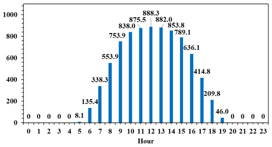
Figure 1.
Average solar irradiance aggregated by hour.
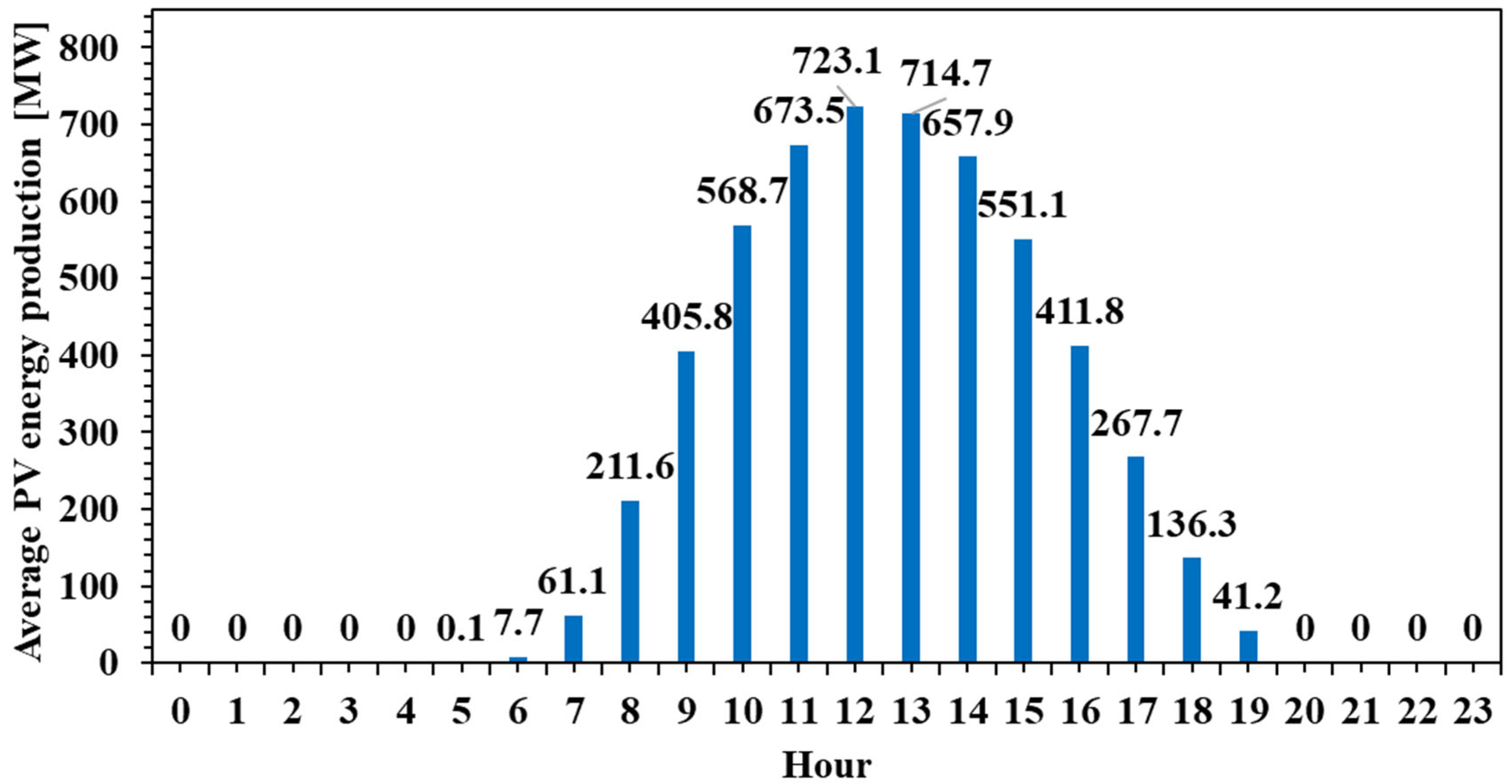
A similar pattern is identified for the actual PV energy production (Figure 2).

Figure 2.
Average PV energy production aggregated by hour.
Both figures display a similar bell-shaped pattern, with values increasing progressively from around 6:00 AM, peaking around midday, and then gradually decreasing towards the evening. The peak solar irradiance reaches approximately 888.3 W/m2 at 12:00 PM, while the peak PV production is recorded slightly earlier, at 11:00 AM, reaching 723.1 MW. This alignment between the two curves confirms the strong dependence of PV output on solar irradiance. However, notable differences in the shape and timing of the curves suggest several important technical insights.
Firstly, the PV production curve is slightly flattened compared to the irradiance curve, indicating that the conversion efficiency of solar energy into electricity is not constant throughout the day. This may be attributed to factors such as thermal effects on the panels, which reduce efficiency under high temperatures, as well as system-level limitations, including inverter capacity or export caps. Moreover, the slight temporal offset between the irradiance peak and the PV output peak reflects the lag caused by the thermal inertia of the panels and potential efficiency degradation during peak sunlight hours.
Secondly, PV output remains nearly zero during the early morning and late afternoon hours, even though some irradiance is present. This suggests that a minimum threshold of solar irradiance is required before significant power generation can occur, potentially due to the startup thresholds of the system’s inverters or inefficiencies at low light levels. These periods of non-generation underscore the intermittent nature of solar energy and reinforce the need for complementary solutions to ensure grid stability.
Finally, while the general trends of both figures align well, the fact that not all available solar energy is converted into electricity highlights inherent system losses—optical, thermal, and electrical. In practical terms, this means that the PV systems are subject to real-world operational constraints and should not be dimensioned solely based on theoretical irradiance data.
From a system-level perspective, the data confirms the volatility of PV output and its mismatch with typical electricity demand patterns, which often show peaks in the early morning and late evening. As such, these figures support the argument for integrating energy storage systems (such as batteries) or demand-side management strategies to shift load profiles accordingly. They are particularly relevant for optimizing PV installations in buildings or industrial applications where energy autonomy, cost reduction, and grid relief are key objectives. Furthermore, this type of hourly analysis is essential for designing hybrid systems or for forecasting PV contributions within larger energy systems.
2.2. Theoretical Fundamentals
Artificial neural networks are composed of artificial neurons arranged in layers. An artificial neuron is a mathematical abstraction of a biological neuron. The equations governing the way information is processed on an artificial neuron level are meant to mimic what is believed to be happening in the biological neuron. Recurrent neural networks are a type of artificial neural network built for tasks oriented to sequence data, such as time series. With built-in features designed to keep knowledge from previous time steps, the prerequisites for achieving good performance are met [28]. In their standard format, there is a possibility of encountering challenges during training, like information morphing, vanishing, or exploding gradients. To avoid these kinds of issues, the Long Short-Term Memory architecture has been proposed [29]. Like standard recurrent neural networks, Long Short-Term Memory maintains the capabilities of keeping time dependencies, but by implementing a gating system. LSTM’s gating system consists of three gates: input, output, and forget (Figure 3). These three gates are neural networks, and the fourth neural network is represented by the hidden state.
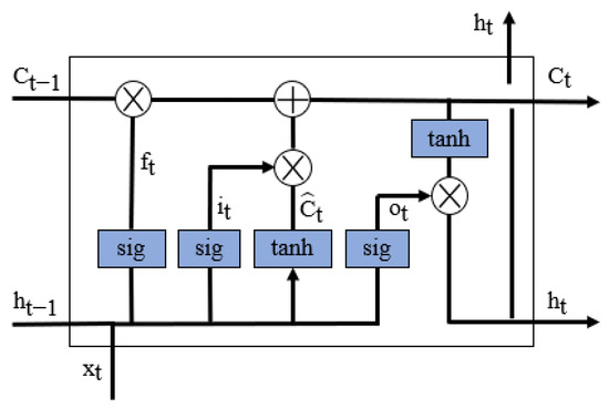
Figure 3.
LSTM architecture. Where is element-wise multiplication and is element-wise addition.
When the information passes through the gates, it is decided what is kept and what is discarded. Since the gates are governed by sigmoid activation functions, the output is bounded between 0 and 1. This means that when the values are close to 0, the information is discarded; when the values are close to 1, the information is kept.
The forget gate’s purpose is to discard unimportant information from the previous cell (Equation (1)).
where is the weight matrix of the current state input, is the weight matrix of the previous cell’s hidden state, t and t−1 are the current time step and the previous time step, respectively, is the current time step input, and is the previous cell’s hidden state.
Comparably, the information is selected in the input gate (Equation (2)):
where and are the weight matrices of the current state input and the previous cell’s hidden state for the input gate, respectively.
The current cell state candidate, , is a temporary value that the cell state can take (Equation (3)):
where the activation function and hyperbolic tangent limit the possible outputs between 1 and 1.
The cell state at the current time step, , is calculated based on the information that is discarded from the previous time step cell state and on the input information acquired at the current time step (Equation (4)):
The output gate controls the information leaving the LSTM cell:
First, the information that is passed through the output gate is calculated (Equation (5)). Second, the information of the calculated cell state (Equation (4)) is regulated using the tanh activation function and then multiplied by the already calculated values in the output gate (Equation (6)):
By design, the cell state at the current time step, , represents long-term memory, while the hidden state at the current time step, represents short-term memory. One of the downsides of this design is that, due to the complex gating system implemented, it is expected to require a high amount of computational power.
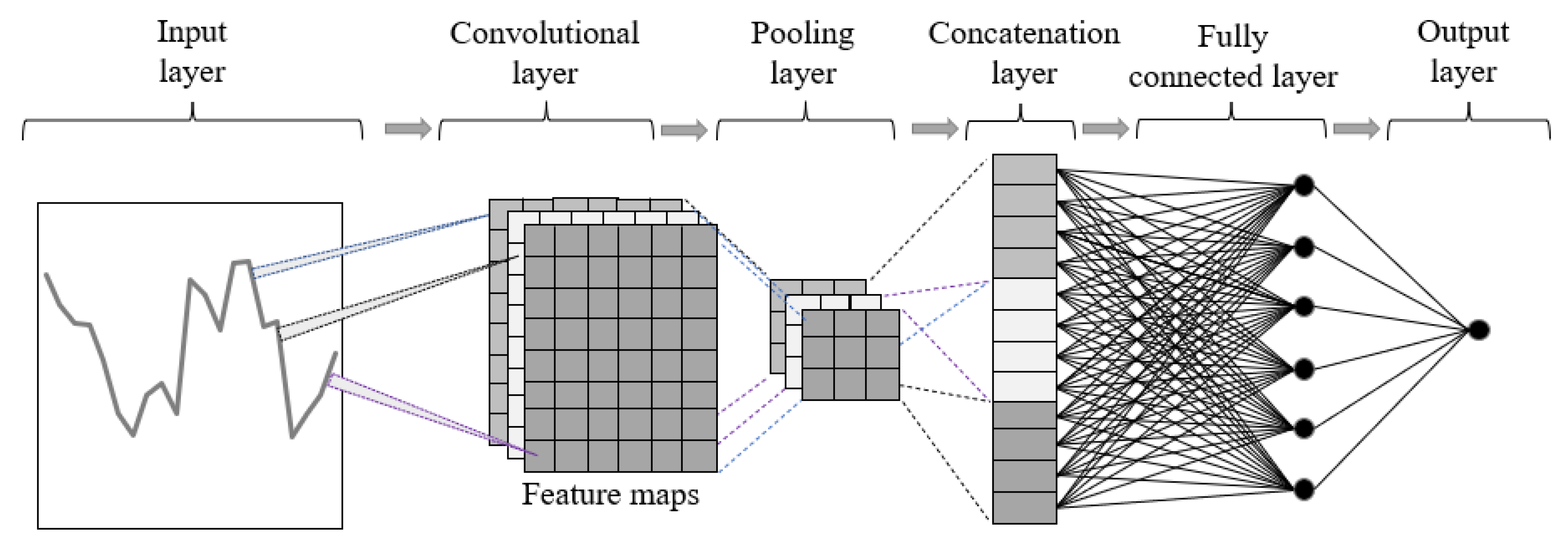
Convolutional neural networks represent a type of model proposed for computer vision. The first task where they were implemented was handwritten digit recognition [30]. Through continued development on image recognition, recently, one-dimensional convolutional neural networks were used for time series analysis [31]. Later, multivariate time series analysis became feasible for time series analysis using convolutional neural networks. One of the major advantages of convolutional neural networks for time series analysis is the ease of setting up computation parallelization, maximizing the use of graphics processing unit cores. Two-dimensional convolutional neural networks use a two-dimensional matrix for input. Usually, convolutional neural networks used for 2D time series analysis consist of an input layer, a convolutional layer, a pooling layer, a concatenation layer, a fully connected layer, and an output layer (Figure 4).
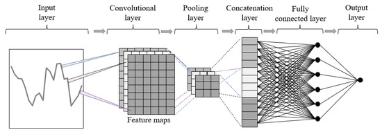
Figure 4.
2D CNN architecture for time series analysis.
In the context of time series analysis, convolution means multiplying the matrix of input data with the two-dimensional matrix of input weights, also known as the kernel [32]. The kernel is moved across the input data in horizontal and vertical directions, capturing it in different ways by having a different position while overlapping. Usually, multiple convolution kernels are used to extract features from the input data. Most of the calculations required by this architecture are completed during this process. The refined convolution calculation of the 2D CNN configuration is as follows [33]:
where is the input value in the input matrix found in the i-th row and j-th column, is the value of the element in the feature map found in the i-th row and j-th column, k is the size of the kernel, and is the value of the weight found in the convolution kernel in the m-th row and n-th column. The pooling layer summarizes the features of each region of the feature map generated by the convolution layer. By summarizing the features, the model’s robustness increases because it does not rely on precisely positioned features generated by the convolution layer. In the concatenation layer, data coming from upstream is transformed into a unidimensional matrix (flattening). In this way, this information can be used as the input data for the fully connected layer. The fully connected layer works like a feedforward neural network, where y is the output of the 2D CNN model (Equation (8)):
where x is the input vector (concatenation layer), w is the input vector (fully connected layer), and f is the activation function.
The model performance assessment for the two supervised learning models in this research is calculated based on the testing subsets. In the case of supervised learning, the predictions are compared to actual values. By using mean absolute error (MAE) and the coefficient of determination (, predictions can be put into context. MAE (Equation (9)) is dependent on the data used. MAE averages the absolute values of the prediction errors, providing an understanding of the prediction performance. (Equation (10)) is independent of the used dataset and measures how much of the variability of the outcome can be explained by the model. is bounded between 0 and 1, where a high value indicates suitable performance.
In the end, there is a possibility that the model will have acceptable performance even if is not very high, if subject matter experts consider the MAE to be at a reasonable level with respect to the industry benchmark.
In terms of setting up model building, training, and testing, a few important steps must be taken. First, this research is a typical supervised machine learning use case. This means the target variable is known, so the model is learning by example. For each target variable, y, there is a set of inputs, x, which are used to predict it with the lowest error. Doing so requires splitting the dataset into two different subsets, keeping the temporal dependencies. The two subsets are called training data and testing data. Training data is used by the model to learn the hidden patterns and relationships between input variables, also known as independent variables, and target variables, also known as dependent variables. Usually, training data consists of 70% to 90% of the data, while the remaining amount is used for testing. The performance metrics described above are calculated based on the testing data that is not known to the model since it is not used for training. Each machine learning model is configured mainly based on experience and various types of trial-and-error strategies. Synaptic weights attached to the neuron’s connections are initiated at the beginning of the training, but while the iterative process is ongoing, they are updated towards values that lead to the lowest error or towards an error that is considered reasonable. The other hyperparameters are selected upfront, as in Table 2.
Table 2.
Hyperparameters used for the model optimization.
Due to the different number of hyperparameters that had to be optimized, in the end, 2916 LSTM models and 8737 CNN models were trained and tested.
3. Results and Discussions
LSTM and CNN architectures are designed for applications involving time series. Both performed very well for the use case proposed in this research (Figure 5). A total of 77% of the CNN models that were trained and later tested had an R2 equal to or higher than 0.9, showing how powerful this architecture is for a wide range of hyperparameters. In the case of LSTM, 13% of the models had an R2 equal to or higher than 0.9. This means that there are fewer models with such high performance, so the number of combinations of optimal hyperparameters is significantly less compared to a CNN. This section, divided by subheadings, provides a concise description of the experimental results, their interpretation, and the experimental conclusions that can be drawn.
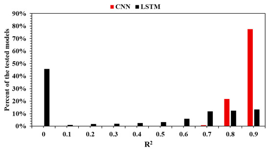
Figure 5.
LSTM vs. CNN performance comparison.
The following observation carries practical implications. When the objective is to develop a high-performing model without exhaustively searching the hyperparameter space, CNNs offer a distinct advantage. The lower success rate of LSTM models suggests that, while these networks may still be capable of excellent results, achieving such performance is more dependent on precise tuning.
Moreover, performance improvements significantly impact the outcome of the decisions made based on the actionable data insights identified. Figure 6 illustrates how the model’s performance is distributed within the R2 range of 0.9 to 0.99.
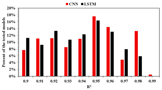
Figure 6.
LSTM vs. CNN performance comparison for models with an equal to or higher than 0.9.
In conclusion, CNNs demonstrate superior robustness and higher potential to achieve strong performance more consistently. LSTM models, while still capable of excellent results, demand more refined hyperparameter optimization. Their performance, although not as uniformly high, may still be competitive in targeted applications when carefully trained.
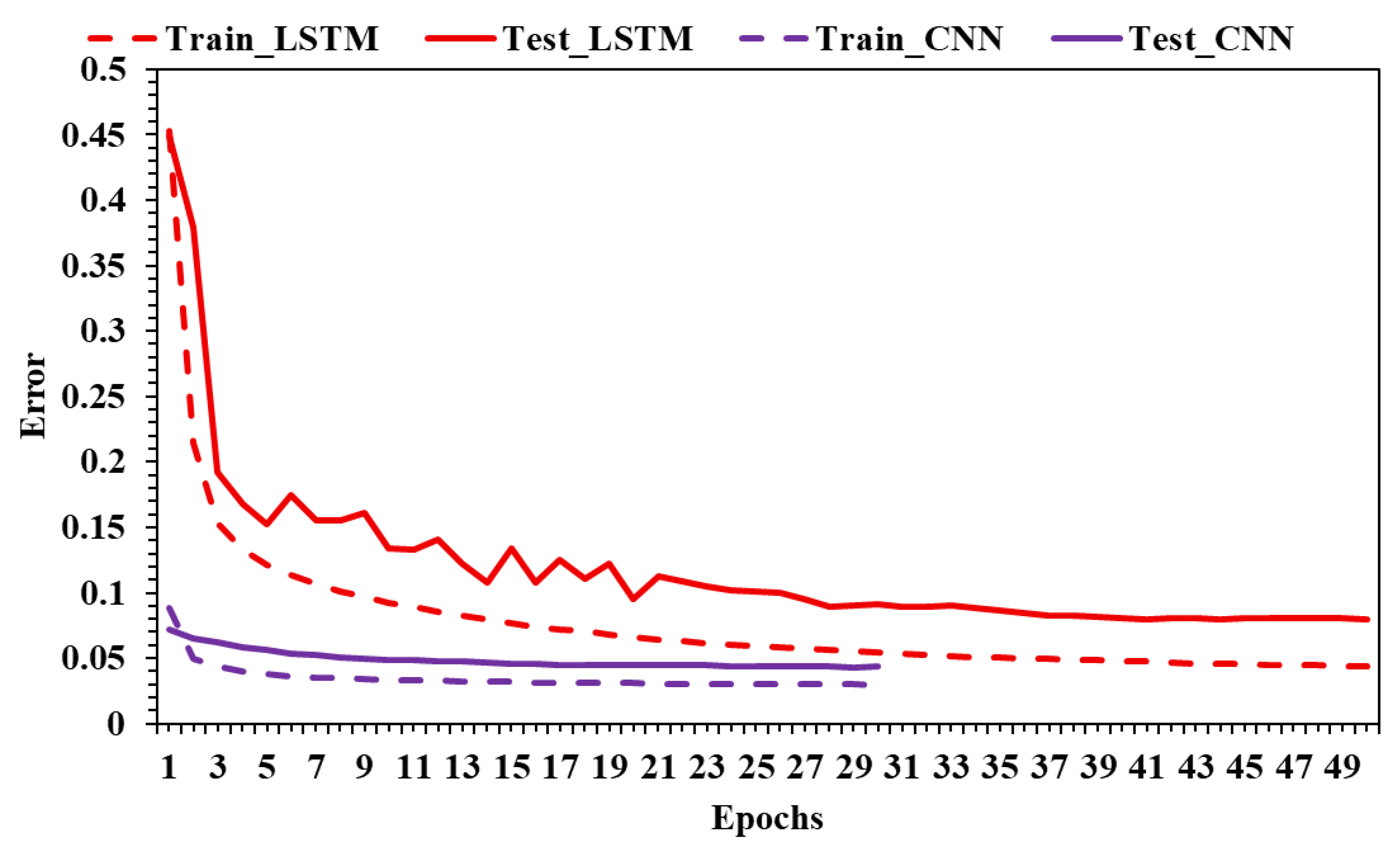
The learning process can be evaluated by analyzing the learning curves generated for each trained model. In Figure 7, there are two curves for the best LSTM and CNN models. The dashed curve shows how the error is evolving epoch by epoch on the training data subset. When the error decreases after consecutive iterations, it means the model can generalize better. The solid line is the error by iteration on the testing data subset. Usually, the error calculated during the training is lower than the error calculated during the test. In the case of CNNs, the training is shorter, and the model converges faster to a stable error and a better performance.
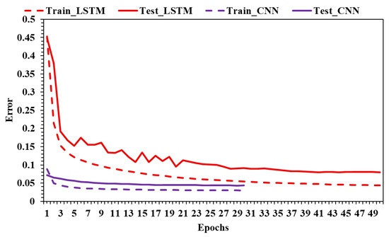
Figure 7.
LSTM vs. CNN learning curves.
There is a clear contrast in the learning dynamics of the two architectures. The CNN model achieves a fast and smooth convergence to a low, stable error within just a few epochs. The proximity between training and testing curves indicates efficient learning and strong generalization, suggesting that the CNN is capable of capturing relevant patterns quickly without overfitting. The training is short, the convergence is early, and the performance is consistent across both datasets.
In contrast, the LSTM model exhibits a higher and more volatile testing error, especially in early epochs. Although the training error decreases steadily, the testing error shows significant fluctuations and takes longer to stabilize. The gap between training and testing error for LSTM is more pronounced, indicating either a risk of overfitting or increased sensitivity to model configuration and temporal sequence complexity.
Overall, Figure 7 demonstrates that the CNN not only learns faster but also generalizes better, making it a more robust and efficient option for time series regression tasks in this specific use case.
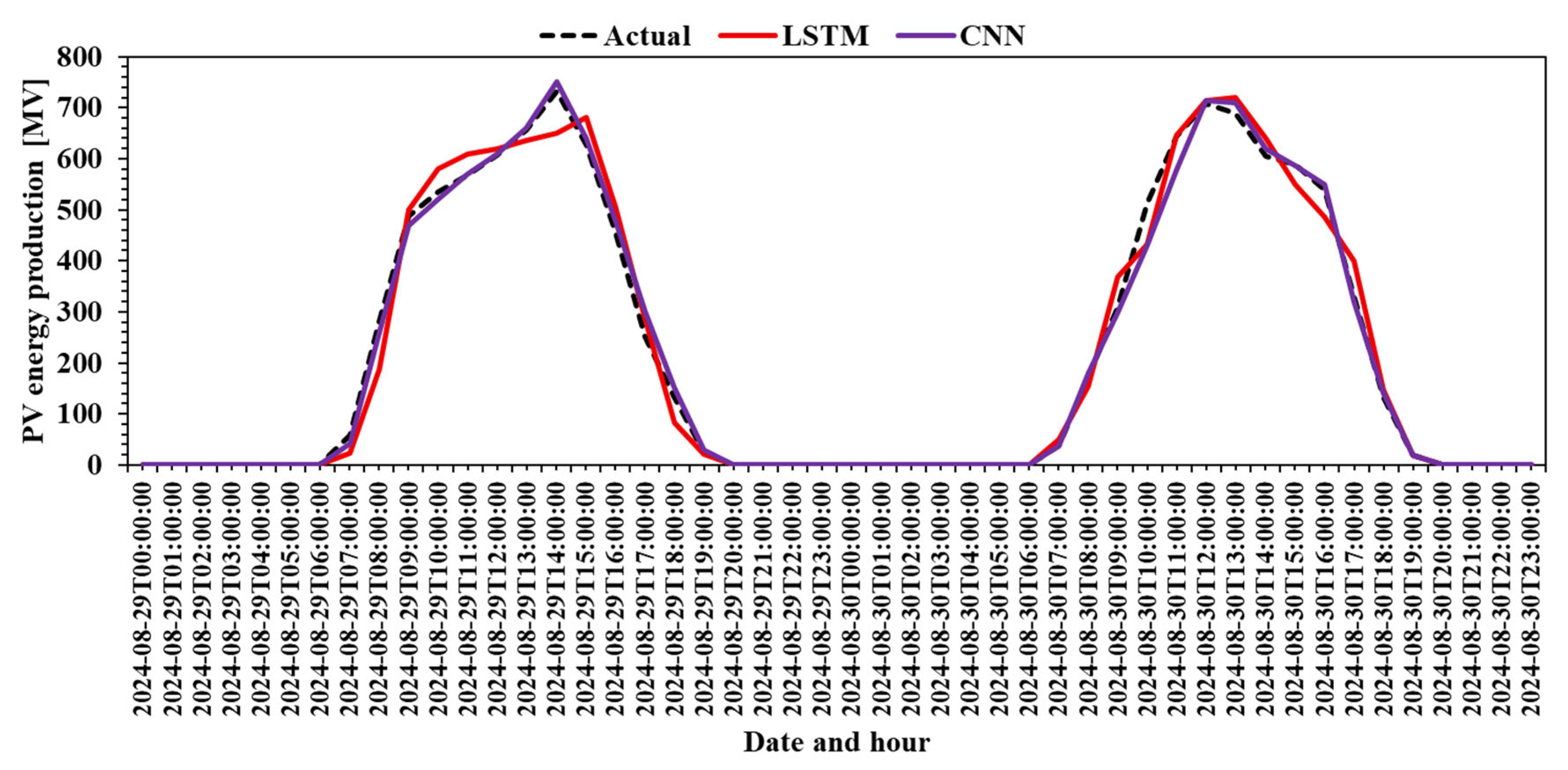
The final assessment on the testing subset is graphed with the actual PV production plotted against the predicted production using LSTM and a CNN (Figure 8). Both models provide very good performance, but as the metrics show, the CNN is better than the LSTM, with the prediction almost overlapping with the actual values of production.
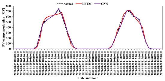
Figure 8.
Actual PV production vs. LSTM prediction vs. CNN prediction.
Figure 8 provides a critical comparison between the actual PV production and the predictions made by LSTM and CNN models during the testing phase. The dashed line represents the ground truth data, while the solid red and purple lines represent the LSTM and CNN predictions, respectively.
At first glance, both models can track the overall shape and pattern of the actual production curve, indicating a strong modeling capacity for diurnal solar energy dynamics. However, the CNN model clearly outperforms LSTM in precision, as its prediction curve aligns almost perfectly with the real data, especially during the rapid rise and fall periods around peak generation hours.
While LSTM performs reasonably well, it shows slightly larger deviations, particularly during transitions, where it may lag behind the true values or smooth out rapid changes. This behavior suggests a lower temporal resolution or delayed response in capturing non-linear variations. The CNN, by contrast, delivers highly accurate, fine-grained predictions, reinforcing its superior modeling of sharp transitions and peak periods.
This figure strongly supports the conclusion drawn earlier from the learning curves: the CNN not only trains more efficiently but also delivers better predictive accuracy, making it a highly reliable choice for time-sensitive PV forecasting applications.
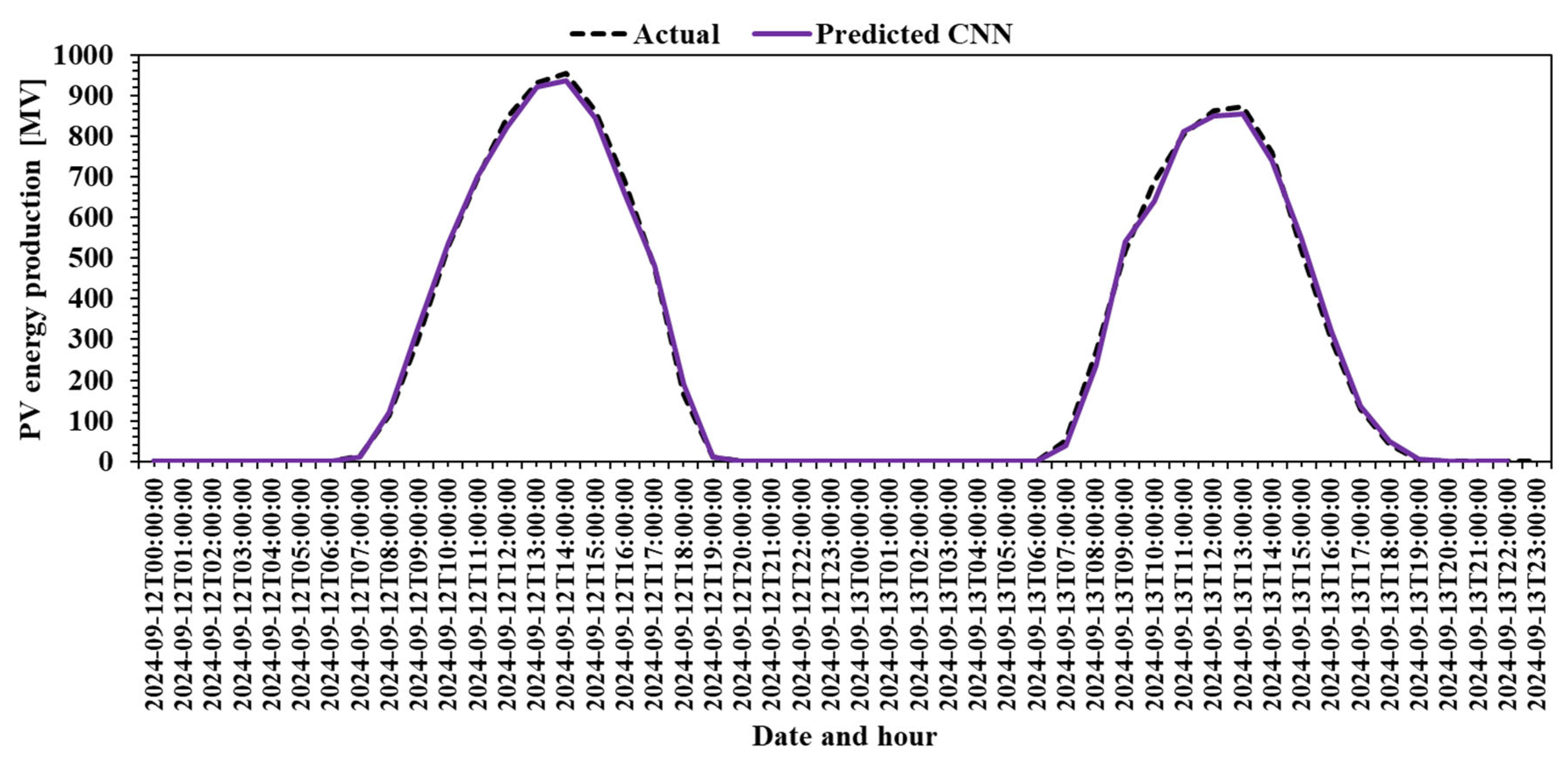
To simulate a real-world scenario, Figure 9 plots the actual PV production against the CNN prediction for a two-day timeframe, 12 September 2024 and 13 September 2024, that was not part of the initial dataset. This confirms the model’s generalization capabilities.
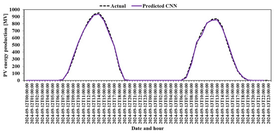
Figure 9.
Model assessment in a real-world scenario.
Figure 9 presents a more rigorous validation of the CNN model by testing its predictions on a real-world simulation scenario. Here, the model is asked to predict PV production for two days (12–13 September 2024) that were excluded from the initial training and testing dataset. This tests the model’s generalization capabilities beyond known data.
The predicted curve (purple) closely overlaps the actual production curve (dashed), showing virtually no significant deviation. This confirms that the CNN model is not simply memorizing historical patterns but has effectively learned the underlying dynamics of solar generation, enabling it to extrapolate accurately to new, unseen data.
This kind of validation is crucial in assessing a model’s robustness for real-world deployment. The CNN’s performance in Figure 9 confirms its reliability under operational conditions, where unknown external factors may affect production. The model’s ability to maintain high accuracy on unseen days is strong evidence of its practical value for forecasting and grid integration.
In comparison with related works, our findings align with those of Etxegarai et al. [15], who also reported better performance of CNNs over LSTMs in intra-hour solar irradiance forecasting. Similarly, Wu et al. [19] demonstrated that transformer-based and convolutional approaches surpass recurrent ones in predictive accuracy for short-term PV output. Unlike studies such as Sulaiman et al. [13], which focus on rooftop systems with rich electrical input data, our work emphasizes the scalability of meteorology-driven forecasts applicable at the national level. Furthermore, our CNN model’s R2 of 0.9913 exceeds the benchmarks reported by Bellagarda et al. [16] and Goutte et al. [11], where R2 values typically range between 0.95 and 0.98 for comparable prediction horizons.
These comparisons support the conclusion that CNNs are particularly well-suited for short-term PV forecasting tasks relying on atmospheric and irradiance data alone. This insight enhances the scientific contribution of the present study, providing not only empirical evidence but also a physically grounded rationale for the observed results.
4. Conclusions
LSTM and CNNs are powerful architectures for PV energy production prediction. For the use case presented in this research, the CNN proved to have a wider range of hyperparameters for which the performance is maximum or close to maximum.
PV energy prediction will remain an open topic due to its importance in the transition to clean energy. The intermittent nature of this energy source is another element that adds volatility to the grid. By accurately predicting it, the volatility added will remain, but the operators will know how to mitigate it. It is worth mentioning that implementing such a prediction system is an effort on the operator’s side, but it brings benefits in addressing issues such as low inertia. However, network stability modeling is a distinct topic that must be addressed accordingly. Future research may consider dust covers for PV panels and explore how to lengthen their lifespan. If the PV panels are not clean, then their performance will drop, and so will the actual energy production. Without having a variable to take into consideration in this scenario, the model will have a tendency to overestimate the energy production. The same is applicable in the case of aging panels, where the wear is reducing their capability of transforming solar irradiation into electricity. Nevertheless, the performance of the existing models is very high and reasonable, but any incremental increase in performance is important for business.
The study highlights the effectiveness of LSTM and CNN architectures for time series applications, particularly in predicting photovoltaic energy production. The results demonstrate that CNN models significantly outperform LSTM models, with 77% of CNN models achieving an R2 of 0.9 or higher, compared to only 13% of LSTM models. This disparity indicates that CNNs are more robust across a wider range of hyperparameters, leading to a greater number of optimal configurations.
When evaluating model performance, the best CNN model achieved an R2 of 0.9913 with a mean absolute error (MAE) of 9.74, whereas the best LSTM model reached an R2 of 0.9880 with an MAE of 12.57. This context underscores the importance of achieving high-performance metrics, as lower error rates directly impact the quality of actionable data insights.
The learning curves for both architectures reveal that the CNN model converges more quickly to a stable error compared to LSTM, indicating better generalization capabilities. The final assessment illustrated in the prediction graphs shows that the CNN’s predictions closely align with actual PV production values, further validating its superior performance. Additionally, the model’s ability to accurately predict PV production over a two-day timeframe not included in the training dataset demonstrates its robustness and generalization capabilities, reinforcing the utility of CNN architectures in real-world applications for photovoltaic energy forecasting.
Author Contributions
Conceptualization, G.C. and V.S.; methodology, G.C., A.-N.B. and V.S.; software, A.-N.B.; validation, G.C., A.-N.B. and V.S.; writing—original draft preparation, G.C., A.-N.B. and V.S.; writing—review and editing, G.C., A.-N.B. and V.S. All authors have read and agreed to the published version of the manuscript.
Funding
This research received no external funding.
Data Availability Statement
Data are available on request to the corresponding author. The data are not publicly available due to the IPR agreement signed by the authors with the funding institution. All data to be made public must undergo the institution’s internal check and approval.
Conflicts of Interest
The authors declare no conflicts of interest.
References
- Arun, M.; Le, T.T.; Barik, D.; Sharma, P.; Osman, S.M.; Huynh, V.K.; Kowalski, J.; Dong, V.H.; Le, V.V. Deep learning-enabled integration of renewable energy sources through photovoltaics in buildings. Case Stud. Therm. Eng. 2024, 61, 105115. [Google Scholar] [CrossRef]
- Iyke, B.N. Climate change, energy security risk, and clean energy investment. Energy Econ. 2024, 129, 107225. [Google Scholar] [CrossRef]
- Miyake, S.; Teske, S.; Rispler, J.; Feenstra, M. Solar and wind energy potential under land-resource constrained conditions in the Group of Twenty (G20). Renew. Sustain. Energy Rev. 2024, 202, 114622. [Google Scholar] [CrossRef]
- Sánchez-Balseca, J.; Pineiros, J.L.; Pérez-Foguet, A. Influence of environmental factors on the power produced by photovoltaic panels artificially weathered. Renew. Sustain. Energy Rev. 2023, 188, 113831. [Google Scholar] [CrossRef]
- Javaid, A.; Sajid, M.; Uddin, E.; Waqas, A.; Ayaz, Y. Sustainable urban energy solutions: Forecasting energy production for hybrid solar-wind systems. Energy Convers. Manag. 2024, 302, 118120. [Google Scholar] [CrossRef]
- Khurshid, H.; Mohammed, B.S.; Al-Yacouby, A.M.; Liew, M.S.; Zawawi, N.A.W.A. Analysis of hybrid offshore renewable energy sources for power generation: A literature review of hybrid solar, wind, and waves energy systems. Dev. Built Environ. 2024, 19, 100497. [Google Scholar] [CrossRef]
- Liu, B.; Wang, H.; Liang, X.; Wang, Y.; Feng, Z. Recycling to alleviate the gap between supply and demand of raw materials in China’s photovoltaic industry. Resour. Conserv. Recycl. 2024, 201, 107324. [Google Scholar] [CrossRef]
- Wazirali, R.; Yaghoubi, E.; Abujazar, M.S.S.; Ahmad, R.; Vakili, A.H. State-of-the-art review on energy and load forecasting in microgrids using artificial neural networks, machine learning, and deep learning techniques. Electr. Power Syst. Res. 2023, 225, 109792. [Google Scholar] [CrossRef]
- Shadmani, A.; Nikoo, M.R.; Gandomi, A.H.; Wang, R.-Q.; Golparvar, B. A review of machine learning and deep learning applications in wave energy forecasting and WEC optimization. Energy Strategy Rev. 2023, 49, 101180. [Google Scholar] [CrossRef]
- Zaidi, A. A bibliometric analysis of machine learning techniques in photovoltaic cells and solar energy (2014–2022). Energy Rep. 2024, 11, 2768–2779. [Google Scholar] [CrossRef]
- Goutte, S.; Klotzner, K.; Le, H.-V.; von Mettenheim, H.-J. Forecasting photovoltaic production with neural networks and weather features. Energy Econ. 2024, 139, 107884. [Google Scholar] [CrossRef]
- Natarajan, Y.; Kannan, S.; Selvaraj, C.; Mohanty, S.N. Forecasting energy generation in large photovoltaic plants using radial belief neural network. Sustain. Comput. Inform. Syst. 2021, 31, 100578. [Google Scholar] [CrossRef]
- Sulaiman, M.H.; Jadin, M.S.; Mustaffa, Z.; Daniyal, H.; Azlan, M.N.M. Short-term forecasting of rooftop retrofitted photovoltaic power generation using machine learning. J. Build. Eng. 2024, 94, 109948. [Google Scholar] [CrossRef]
- Almeshaiei, E.; Al-Habaibeh, A.; Shakmak, B. Rapid evaluation of micro-scale photovoltaic solar energy systems using empirical methods combined with deep learning neural networks to support systems’ manufacturers. J. Clean. Prod. 2020, 244, 118788. [Google Scholar] [CrossRef]
- Etxegarai, G.; López, A.; Aginako, N.; Rodríguez, F. An analysis of different deep learning neural networks for intra-hour solar irradiation forecasting to compute solar photovoltaic generators’ energy production. Energy Sustain. Dev. 2022, 68, 1–17. [Google Scholar] [CrossRef]
- Bellagarda, A.; Grassi, D.; Aliberti, A.; Bottaccioli, L.; Macii, A.; Patti, E. Effectiveness of neural networks and transfer learning to forecast photovoltaic power production. Appl. Soft Comput. 2023, 149, 110988. [Google Scholar] [CrossRef]
- de Souza Silva, J.L.; Mahmoudi, E.; Carvalho, R.R.M.; Barros, T.A.D.S. Classification of anomalies in photovoltaic systems using supervised machine learning techniques and real data. Energy Rep. 2024, 11, 4642–4656. [Google Scholar] [CrossRef]
- Hou, Z.; Zhang, Y.; Liu, Q.; Ye, X. A hybrid machine learning forecasting model for photovoltaic power. Energy Rep. 2024, 11, 5125–5138. [Google Scholar] [CrossRef]
- Wu, J.; Zhao, Y.; Zhang, R.; Li, X.; Wu, Y. Application of three Transformer neural networks for short-term photovoltaic power prediction: A case study. Sol. Compass 2024, 12, 100089. [Google Scholar] [CrossRef]
- Sulaiman, M.H.; Jadin, M.S.; Mustaffa, Z.; Azlan, M.N.M.; Daniyal, H. Short-Term forecasting of floating photovoltaic power generation using machine learning models. Clean. Energy Syst. 2024, 9, 100137. [Google Scholar] [CrossRef]
- Jai, A.A.; Ouassaid, M. Three novel machine learning-based adaptive controllers for a photovoltaic shunt active power filter performance enhancement. Sci. Afr. 2024, 24, e02171. [Google Scholar] [CrossRef]
- Oprea, S.-V.; Bâra, A. Ultra-short-term forecasting for photovoltaic power plants and real-time key performance indicators analysis with big data solutions. Two case studies—PV Agigea and PV Giurgiu located in Romania. Comput. Ind. 2020, 120, 103230. [Google Scholar] [CrossRef]
- Năstase, G.; Șerban, A.; Dragomir, G.; Brezeanu, A.I.; Bucur, I. Photovoltaic development in Romania. Reviewing what has been done. Renew. Sustain. Energy Rev. 2018, 94, 523–535. [Google Scholar] [CrossRef]
- Prăvălie, R.; Sîrodoev, I.; Ruiz-Arias, J.; Dumitraşcu, M. Using renewable (solar) energy as a sustainable management pathway of lands highly sensitive to degradation in Romania. A countrywide analysis based on exploring the geographical and technical solar potentials. Renew. Energy 2022, 193, 976–990. [Google Scholar] [CrossRef]
- Vrînceanu, A.; Dumitrașcu, M.; Kucsicsa, G. Site suitability for photovoltaic farms and current investment in Romania. Renew. Energy 2022, 187, 320–330. [Google Scholar] [CrossRef]
- Visual Crossing Weather Data. 2024. Available online: https://www.visualcrossing.com/resources/documentation/weather-data/weather-data-documentation/ (accessed on 14 September 2024).
- Available online: https://www.transelectrica.ro/widget/web/tel/sen-grafic/-/SENGrafic_WAR_SENGraficportlet (accessed on 14 September 2024).
- Pascanu, R.; Gulcehre, C.; Cho, K.; Bengio, Y. How to construct deep recurrent neural networks. In Proceedings of the Second International Conference on Learning Representations (ICLR 2014), Banff, AB, Canada, 14–16 April 2014. [Google Scholar]
- Hochreiter, S.; Schmidhuber, J. Long Short-term Memory. Neural Comput. 1997, 9, 1735–1780. [Google Scholar] [CrossRef]
- Le Cun, Y.; Boser, B.; Denker, J.S.; Henderson, D.; Howard, R.E.; Hubbard, W.; Jackel, L.D. Handwritten Digit Recognition with a Back-Propagation Network. In Proceedings of the Advances in Neural Information Processing Systems (NIPS 1989), Denver, CO, USA, 27–30 November 1989; Morgan Kaufmann: Burlington, MA, USA, 1990. [Google Scholar]
- Zhang, A.; Lipton, Z.C.; Li, M.; Smola, A.J. Dive into Deep Learning. 2020. Available online: https://d2l.ai/chapter_convolutional-neural-networks/index.html (accessed on 2 January 2024).
- Rohrer, B. Convolution in One Dimension for Neural Networks [Interactiv]. 2020. Available online: https://e2eml.school/convolution_one_d.html (accessed on 22 December 2023).
- Kiranyaz, S. 1D convolutional neural networks and applications: A survey. Mech. Syst. Signal Process. 2021, 151, 107398. [Google Scholar] [CrossRef]


Disclaimer/Publisher’s Note: The statements, opinions and data contained in all publications are solely those of the individual author(s) and contributor(s) and not of MDPI and/or the editor(s). MDPI and/or the editor(s) disclaim responsibility for any injury to people or property resulting from any ideas, methods, instructions or products referred to in the content. |
© 2025 by the authors. Licensee MDPI, Basel, Switzerland. This article is an open access article distributed under the terms and conditions of the Creative Commons Attribution (CC BY) license (https://creativecommons.org/licenses/by/4.0/).