Deep Learning-Based Method for Operation Dispatch Strategy Generation of Virtual Power Plants

Abstract

Centralized and distributed optimization methods used by traditional virtual power plants (VPPs) in power system dispatching face issues such as high computational complexity, difficulties in privacy protection, and slow iterative convergence. There is an urgent need to propose an accurate and efficient acceleration method for generating VPP operational dispatching strategies. This paper proposes a deep learning-based acceleration method for generating VPP operational dispatching strategies. By using the equivalent projection method to solve the operation feasible region of the VPP, the objective function and constraints of the VPP are transformed into constraints of coordination variables and submitted to the system dispatching center for optimization, thereby avoiding the slow convergence problem of iterative computation methods. The Kolmogorov–Arnold Network (KAN) is employed to predict the batch operation feasible regions of the VPP, addressing the inefficiency of individually calculating feasible regions. Tests on a 13,659-node system show that the proposed method reduces solution time by 64.40% while increasing the objective function value by only 4.74%, verifying its accuracy and speed.

1. Introduction

VPPs aggregate distributed energy resources (DERs) to extract their energy value, provide generation capacity, and participate in the main grid dispatch, thereby achieving the optimized allocation of distributed resources. This characteristic has attracted much attention. Utilizing smart metering and communication technologies, VPPs can integrate a large number of renewable energy resources distributed across the distribution network, providing adjustable capabilities similar to conventional units, reducing the complexity of grid optimization, promoting the participation of distributed new energy, and enhancing the economic and flexible operation of the grid [1,2,3,4].

Traditional VPP scheduling typically employs centralized optimization dispatch [5] or distributed dispatch [6] methods. Centralized optimization requires the grid’s unified dispatch center to collect all equipment parameter information for optimization, but raises privacy protection concerns. Although distributed optimization can safeguard user privacy and reduce computational pressure on the dispatch center, it necessitates multiple iterative solutions, suffering from slow convergence—making it difficult to meet the timeliness requirements of VPP rapid response. Particularly, when the system contains numerous binary variables such as start-stop units, existing solution methods face computational efficiency bottlenecks [7,8].

To meet the timeliness requirements of VPP rapid response [9], there is an urgent need to develop novel fast scheduling methods. Existing approaches, such as improved cooperative particle swarm optimization algorithms [10], genetic algorithms [11], and joint market temporal rolling bidding strategies [12], exhibit limited convergence in enhancing scheduling speed.

The feasible region projection method proposed in [13,14], significantly improves computational efficiency by transforming the constraint set of lower-level equipment into boundary conditions for upper-level scheduling, thereby reducing the original bilevel optimization problem to a single-layer formulation. Similarly, studies [15,16,17] leverage the scheduling boundaries of lower-level models for collaborative optimization. Building upon these advancements, this paper innovatively proposes an accelerated scheduling strategy generation method based on the operation feasible region of VPPs.

Recently, ML and DL techniques have gained increasing attention in VPP scheduling due to their ability to model nonlinear dynamics and adapt to real-time data. For instance, Ref. [18] employed deep reinforcement learning to co-optimize multiple VPP objectives under uncertain renewable conditions. Other works [19,20] have explored graph neural networks, hybrid optimization-ML frameworks, and deep surrogate models to approximate VPP flexibility, improve convergence speed, and reduce reliance on detailed physical models. Despite these advances, many existing methods suffer from high training costs or lack interpretability, motivating the need for efficient and explainable VPP decision frameworks.

This paper proposes an accelerated scheduling strategy generation method based on the operation feasible regions of VPP. The approach first employs an equivalent projection method to generate VPP’s operation feasible regions in real-time, aggregating distributed resource constraints into schedulable boundaries. Subsequently, it trains a KAN network-based feasible region predictor to batch-generate time-varying feasible regions for multiple VPPs. Compared with traditional Multilayer Perceptrons (MLPs), the KAN network achieves superior parameter efficiency and prediction accuracy through learnable activation functions [21]. This innovation enables the dispatch center to rapidly acquire information about the entire grid’s adjustable resources.

Key innovations of this study include the following:

• Constructing a dynamic feasible region scheduling model for VPPs, which converts distributed optimization into centralized scheduling under feasible region constraints, eliminating iterative computations.
• Developing a KAN network-based feasible region prediction framework to enable fast and accurate updates of multi-VPP feasible regions.

Research Hypothesis. We hypothesize that the integration of equivalent projection and KAN-based learning can accelerate VPP operation strategy generation, significantly reducing computational burden while preserving dispatch feasibility and decision quality. This hypothesis is evaluated through comparative experiments in Section 4.

This paper is organized as follows: Section 2 details the VPP dispatching model, Section 3 introduces the proposed accelerated method, Section 4 presents the case study, Section 5 discusses the results, and Section 6 concludes the paper. The Appendix A provides detailed parameters.

2. VPP Dispatching Model

As illustrated in Figure 1, the proposed workflow consists of three main stages: (i) physical constraint projection, (ii) learning-based feasible region approximation, and (iii) dispatch decision. Local-level constraints—including power balance, device limits, and renewable uncertainty—are first projected into a boundary representation via equivalent projection. Labeled samples are then generated (feasible/infeasible), forming the training dataset for the Kolmogorov–Arnold Network (KAN). Once trained, the KAN model serves as a fast feasibility classifier, supporting real-time dispatch by filtering infeasible actions and accelerating optimization.

2.1. Dispatching Center Optimization Model

In this study, the model focuses exclusively on the active power dispatch and its corresponding feasible region under fixed electricity prices. Reactive power balance and voltage constraints are not explicitly modeled, and all prices are assumed constant over the dispatch horizon. This simplification allows us to isolate the geometric and computational aspects of feasible region learning without entanglement with market dynamics or AC power flow effects.

Generally, the dispatching center model aims at achieving optimal economic efficiency for the entire grid, which can be formulated as follows:

$$min\sum _{t\in T}\left(\sum _{g\in G}{\lambda }_g{P}_{g,t}+\sum _{w\in W}{c}_w{P}_{c,w,t}+\sum _{s\in S}{c}_s{P}_{c,s,t}+\sum _{v\in V}{\pi }_{v,t}^{VPP}\right)$$

(1)

subject to the following:

$$\sum _{g\in G}{G}_{g,r}{P}_{g,t}^{TN}+\sum _{w\in W}{W}_{w,r}{P}_{w,t}^{TN}+\sum _{s\in S}{S}_{s,r}{P}_{s,t}^{TN}=D_{r,t}^{TN}+P_{r,t}^{TN,in},\forall r\in R,\forall t\in T$$

(2)

$$P_{r,t}^{TN,in}=\sum _{n\in R}{B}_{r,n}({\theta }_{r,t}-{\theta }_{n,t}),\forall r\in R,\forall t\in T$$

(3)

$${\mu }_{g,t}{P}_{g,t}^{TN,min}\le P_{g,t}^{TN}\le {\mu }_{g,t}{P}_{g,t}^{TN,max},\forall g\in G,\forall t\in T$$

(4)

$$P_{g,t+1}^{TN}-P_{g,t}^{TN}\le ({\mu }_{g,t+1}-{\mu }_{g,t})P_g^{TN,min}+P_g^{TN,up},\forall g\in G,\forall t\in T$$

(5)

$$P_{g,t}^{TN}-P_{g,t+1}^{TN}\le ({\mu }_{g,t}-{\mu }_{g,t+1})P_g^{TN,min}+P_g^{TN,down},\forall g\in G,\forall t\in T$$

(6)

$$\sum _{k=t+1}^{k^{on}}{\mu }_{g,k}\ge T_g^{on}({\mu }_{g,t+1}-{\mu }_{g,t}),\forall g\in G,\forall t\in T$$

(7)

$$\sum _{k=t+1}^{k^{off}}{\mu }_{g,k}\le T_g^{off}({\mu }_{g,t+1}-{\mu }_{g,t}),\forall g\in G,\forall t\in T$$

(8)

$$k^{on}=min\{t+T_g^{on},T\}$$

(9)

$$k^{off}=min\{t+T_g^{off},T\}$$

(10)

whereas $P_{g,t}^{TN}$, $P_{c,w,t}^{TN}$ and $P_{c,s,t}^{TN}$ are the output pf thermal power units in the main grid, the curtailed wind power and solar power, respectively, ${\lambda }_g$, $c_w$ and $c_s$ are the cost coefficients for the output of thermal power units and the penalty cost coefficients for abandoning wind and solar, respectively, ${\pi }_{v,t}^{VPP}$ is the operational cost of VPP, $P_{w,t}^{TN}$, $P_{s,t}^{TN}$, are actual wind power output and solar power output, respectively, $G_{g,r}$, $W_{w,r}$ and $S_{s,r}$ are incidence matrices between units, wind farms, solar power plants and nodes, $D_{r,t}^{TN}$ is the node demand at node r, $P_{r,t}^{TN,in}$ is the net injected power at node r, $B_{r,n}$ is the conductance matrix between node i and branch j, ${\theta }_{r,t}$ is the phase angle at node r, and ${\mu }_{g,t}$ is the binary variable representing the on-off status of the thermal power units.

Constraint (2) is the nodal power balance constraint, (3) is the power flow constraint, (4) is the upper and lower limit constraint for the active power output of the units, (5) and (6) are the ramping constraints for the units, and (7) to (10) are the minimum start-up and shut-down time constraints for the units. Due to the presence of binary variables and constraints (4) to (8), the problem becomes a mixed-integer linear programming (MILP) problem, and its solution time increases significantly with the scale of the problem. Therefore, how to accelerate the solution process for the clearing problem of virtual market participation in the electricity market is the focus of this paper.

2.2. VPP Operation and Dispatch Model

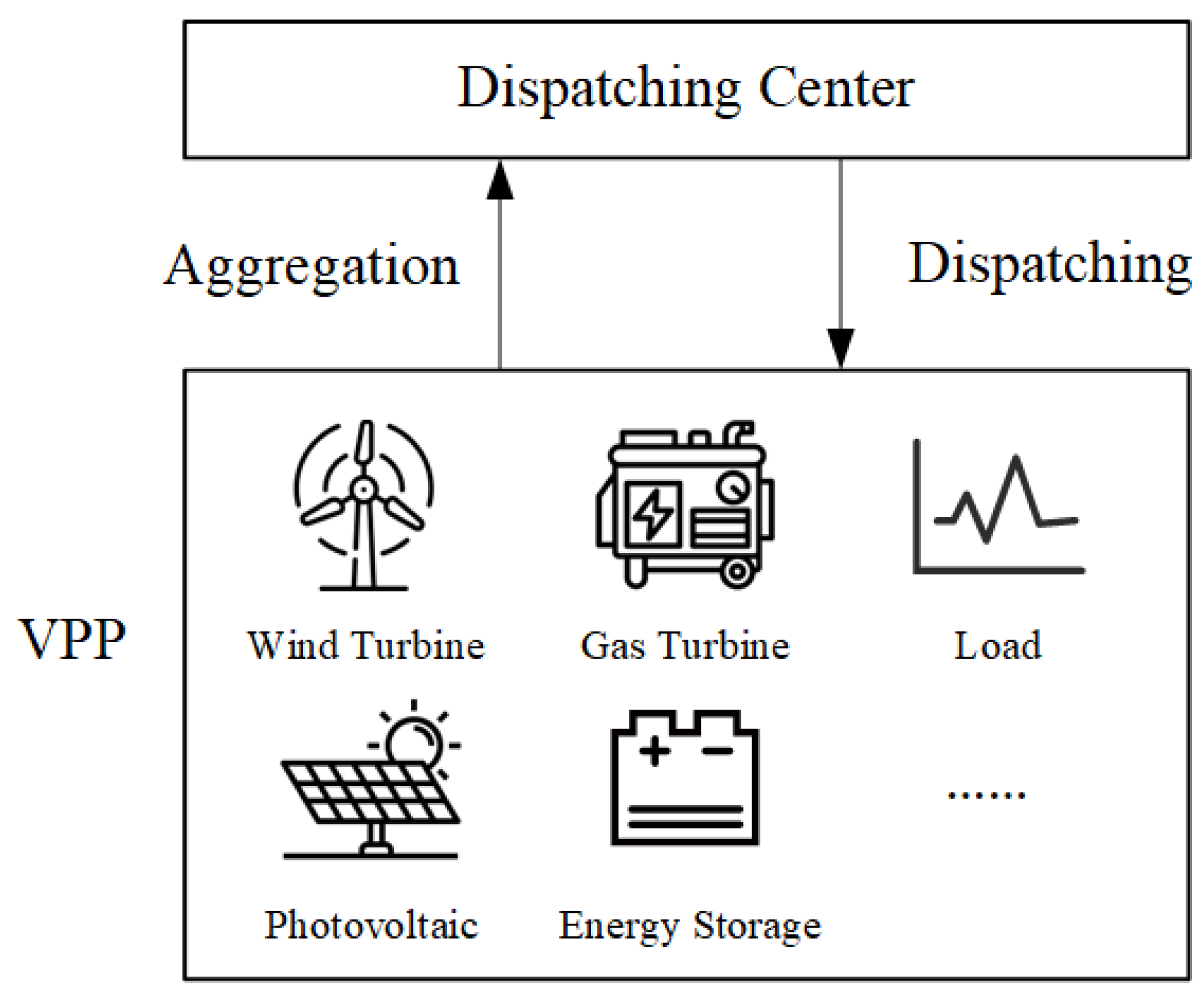
The VPP aggregates a large number of DERs in the distribution network, such as photovoltaic systems, wind power, and controllable units, as shown in Figure 2. It calculates its operation feasible region and reports it to the dispatching center.

The operation feasible region refers to the adjustable range of coordination variables—specifically, the exchanged active power and submitted prices at the VPP boundary nodes—that do not violate internal operational constraints.

Coordination variables are defined as the interface quantities through which a VPP interacts with the main grid, typically including boundary active power injection $P_{o,t}^{VPP}$ and the associated price ${\pi }_{o,t}^{VPP}$ at each scheduling period. These variables are visible to the dispatch center and form the input to system-level optimization.

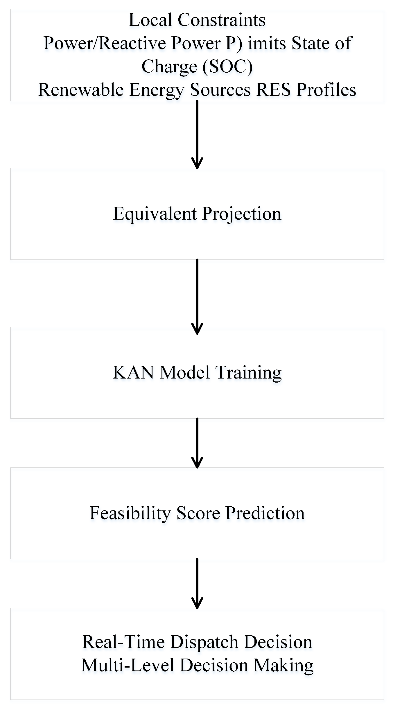
Equivalent projection refers to the process of projecting the high-dimensional internal constraints of the VPP onto the low-dimensional space of coordination variables. This transformation allows the VPP to submit only its boundary feasible region (as a function of coordination variables), thereby enabling centralized scheduling without revealing detailed internal models or solving the full optimization problem online.

Essentially, the VPP dispatch boundary is a dimensionality-reduced mapping of the high-dimensional feasible region of the VPP dispatch model onto the space of boundary node coupling variables. This means that for any point within the feasible region, the VPP can determine a dispatch decision set that does not violate its steady-state constraints.

The VPP submits its operation feasible region to the dispatch center, which then makes optimal dispatch decisions based on this feasible region. After the dispatch center delivers dispatch commands to the VPP, the VPP executes the final decision-making calculations.

By using the equivalent projection method to aggregate massive DERs and requiring the VPP to submit only its operation feasible region information, data privacy of the VPP can be effectively protected.

Typically, the objective function and constraints of the VPP can be expressed as follows.

$$min{\pi }_v^{VPP}=\sum _{t\in T}({\lambda }_{o,t}{P}_{o,t}^{VPP}+\sum _{g\in G}{\lambda }_{g,t}{P}_{g,t}^{VPP}+\sum _{w\in W}{c}_w{P}_{w,t}^{VPP}+\sum _{s\in S}{c}_s{P}_{c,s,t}^{VPP})$$

(11)

subject to the following:

$$P_{n,t}^{VPP}=e_g{P}_{g,t}^{VPP}+e_r{P}_{r,t}^{VPP}-e_d{P}_{d,t}^{VPP}-e_o{P}_{o,t}^{VPP},\forall n\in N,\forall t\in T$$

(12)

$$Q_{n,t}^{VPP}=e_g{P}_{g,t}^{VPP}+e_r{P}_{r,t}^{VPP}-e_d{Q}_{d,t}^{VPP},\forall n\in N,\forall t\in T$$

(13)

$$U_{j,t}-U_{i,t}=-2(r_{ij}{P}_{ij,t}+x_{ij}{Q}_{ij,t})+(r_{ij}^2+x_{ij}^2)l_{ij,t},\forall (i,j)\in E,t\in T$$

(14)

$$l_{ij,t}+u_{i,t}\ge {\parallel 2P_{ij,t},2Q_{ij,t},l_{ij,t}-u_{i,t}\parallel }_2,\forall (i,j)\in E,t\in T$$

(15)

$$P_{ij}^{min}\le P_{ij,t}\le P_{ij}^{max},\forall (i,j)\in E,t\in T$$

(16)

$${\left(U_i^{min}\right)}^2\le u_{i,t}\le {\left(U_i^{max}\right)}^2,\forall i\in N,t\in T$$

(17)

$${\left(I_{ij}^{min}\right)}^2\le l_{ij,t}\le {\left(I_{ij}^{max}\right)}^2,\forall (i,j)\in E,t\in T$$

(18)

$$P_g^{VPP,min}\le P_{g,t}^{VPP}\le P_g^{VPP,max},\forall g\in G,t\in T$$

(19)

$$Q_g^{VPP,min}\le Q_{g,t}^{VPP}\le Q_g^{VPP,max},\forall g\in G,t\in T$$

(20)

where N and E are the node set and branch set of a VPP, respectively; $P_{n,t}^{VPP}$ and $Q_{n,t}^{VPP}$ are active power and reactive power injected into the VPP node at the moment t, respectively; $P_{g,t}^{VPP}$ and $Q_{g,t}^{VPP}$ are the active power and reactive power output of the adjustable unit of the VPP at the moment t, respectively; $P_{r,t}^{VPP}$ and $Q_{r,t}^{VPP}$ are the prediction of the active power and reactive power output of the distributed renewable energy at time t, wherein this paper sets the distributed renewable energy to operate in the mode of constant power factor, namely, the reactive power of the new energy $Q_{r,t}^{VPP}=Diag\left(\tan {\varphi }_R\right)P_{r,t}^{VPP}$ ($tan{\varphi }_R$ is the constant power factor vector of the new energy); $P_{d,t}^{VPP}$ and $Q_{d,t}^{VPP}$ are the active power demand and reactive power demand at time t, respectively; $P_{o,t}^{VPP}$ is the exchange active power at time t at boundary nodes of the VPP; $P_{L,t}^{VPP}$ and $Q_{L,t}^{VPP}$ are the active power and reactive power on the internal branch of the VPP at time t, respectively; $e_G$, $e_R$, $e_D$ and $e_O$ are the incidence matrices of adjustable units, distributed new energy units, loads, and virtual power plant gateway nodes and each node, respectively. $u_{i,t}$ is the square of the voltage amplitude of the node i at time t, $r_{ij}$ and $x_{ij}$ is the resistance and reactance of the branch $(i,j)$, and $P_{ij,t}$, $Q_{ij,t}$ and $l_{ij,t}$ are the active power flow, reactive power flow, and the square of the current amplitude of the branch $(i,j)$ at time t, respectively.

Considering that the long-distance transmission of reactive power in the power grid will affect the voltage quality and lead to the increase of active loss, and the reactive power of the grid often adopts the method of in situ equilibrium, this paper studies the mode of exchanging active power between the boundary nodes of the virtual power plant and the main network, and does not consider the reactive power exchange for the time being, and the coupling variable of the virtual power plant is the exchange of active power at the boundary node. The multi-time scheduling of virtual power plants needs to meet the constraints of node power balance (12) and (13), branch power flow constraints (14) and (15), system state variable constraints (16) to (18), and constraints of the upper and lower output limits of adjustable units (19) and (20).

Since this paper does not consider time-coupled constraints of VPP (such as ramping constraints and energy storage constraints), the VPP’s dispatch optimization problem falls into the category of linear programming problems, which can be solved relatively quickly.

Whether using centralized or distributed algorithms, the dispatch center needs to perform coordinated optimization calculations, which increases the problem scale and solution time. In contrast, the equivalent projection method avoids the joint optimization solving between the virtual power plant and the main grid, thereby improving computational efficiency.

Define two types of variables related to the operational scheduling of VPPs:

• Coupling variables $w_t$: The exchanged active power and quotation at the boundary nodes of the VPP in each time period, namely,
  $w_t={[(P_{o,1}^{VPP},{\pi }_{o,1}^{VPP}),(P_{o,2}^{VPP},{\pi }_{o,2}^{VPP}),\dots ,(P_{o,v}^{VPP},{\pi }_{o,v}^{VPP})]}^T$.
  These variables can be derived from the optimal scheduling of the main network (1) to (10), and are fixed as the boundary condition of the optimization decision of the VPP.
• Internal variables $x_t$:$x_t={[P_{g,t}^{VPP},Q_{g,t}^{VPP},U_t,I_t]}^T$. For the fixed coupling variables $w_t$, the internal variables $x_t$ can be determined by the VPP’s self-scheduling optimization, namely, given $w_t$, the internal variables $x_t$ can be obtained by solving (11) to (20).

Define the feasible operating range of variables that satisfy the constraints of Equations (2)–(8) for the multi-period scheduling of VPPs as $\Phi$, and the multi-period scheduling boundary of VPPs as $\Omega$. For any coupling variable value w on the multi-period scheduling boundary $\Omega$, there exists a set of feasible control and state variables $x_t$ that satisfy the feasible operating range of variables, namely Equation (21):

$$\Omega =\left\{w_t\right|\forall t\in T,\exists x_t,(w_t,x_t)\in \Phi \}$$

(21)

To elaborate on the transformation, the equivalent projection method reduces the original bi-level optimization model into a tractable single-level formulation. Specifically, given a fixed set of boundary (coupling) variables $w_t$, the internal VPP optimization problem (Equations (11)–(20)) can be solved independently to obtain feasible internal states $x_t$. By exploring the entire feasible set $\Phi$ and projecting it onto the $w_t$-space, we obtain the feasible boundary region $\Omega$, which is submitted to the upper-level dispatch center for centralized optimization. This process ensures that the internal device constraints are implicitly satisfied while preserving data privacy.

In contrast to traditional bi-level iterative frameworks, the equivalent projection approach enables each VPP to condense its complex internal constraints into a low-dimensional feasible region defined by boundary coordination variables (e.g., tie-line active power and cost). The projection process involves solving multiple instances of the internal VPP problem to determine the outer convex hull of feasible operating points in the coupling variable space. The resulting region $\Omega$ acts as a constraint set for the upper-level market-clearing problem, thus transforming the original nested optimization into a decoupled and efficient structure.

3. Deep Learning-Based Acceleration Method for Operation and Dispatching of VPP

The proposed method comprises the following steps:

• Training Data Collection: Gather load, wind power, and photovoltaic data, and determine the VPP’s feasible region using the vertex search method.
• KAN Network Training: Train a KAN network using the collected data to predict the VPP’s feasible region.
• VPP Feasible Region Prediction: Utilize the trained KAN network to predict the feasible region for the current time period, enabling batch computation for multiple VPPs.
• Dispatch Center Optimization: The dispatch center performs optimal scheduling based on the submitted predicted feasible regions of the VPPs.
• Execution of Results: The VPP receives dispatch instructions and executes power generation accordingly.

By integrating the equivalent projection method with deep learning techniques, this approach significantly accelerates the VPP dispatch process, addressing the computational efficiency and data privacy challenges inherent in traditional methods while enhancing system flexibility and economic performance. The proposed method not only strengthens the market competitiveness of VPPs but also facilitates the widespread adoption of distributed renewable energy and optimized grid operation.

Commonly used methods for characterizing the operation feasible region include geometric parameter approximation [22], multi-parameter linear programming [23,24], and vertex search [25,26,27]. This paper takes the vertex search method as an example to solve the operation feasible region of VPPs.

3.1. Vertex Search Method

The Equivalent Projection Method is a technique that transforms a VPP’s operation feasible region into constraint conditions for the upper-level model. This method is implemented through the following steps:

First, the VPP’s operation is modeled as an optimization problem aimed at cost minimization while satisfying power system operational constraints. By solving this problem, the VPP’s operation feasible region is determined, which represents the adjustable range of coupling variables between the VPP and the main grid without violating operational constraints.

Subsequently, the VPP’s operation feasible region is projected onto the coupling variable space of the main grid, thereby converting the bi-level optimization problem into a single-level problem. This effectively avoids the slow convergence issue inherent in distributed model iterations.

Under this method, the VPP no longer submits specific generation output and price information to the dispatch center, but rather its operation feasible region information. This approach reduces problem complexity through dimensionality reduction while preserving the privacy of the VPP’s internal operations, ultimately accelerating VPP dispatch calculations.

First, the vertex identification problem is determined as (22).

$$maxh={\alpha }^{T}ws.t.Aw+Bx\le c$$

(22)

where $\alpha$ represents the direction of the vertex search. For solving the operation feasible region of the virtual power plant, the constraints are constraints (12) to (20) and constraints related to the quotation of the virtual power plant (23), where M is a very large positive number.

$$\sum _{t\in T}({\lambda }_{o,t}{P}_{o,t}^{VPP}+\sum _{g\in G}{\lambda }_{g,t}{P}_{g,t}^{VPP}+\sum _{s\in S}{c}_{s,t}{P}_{s,t}^{VPP})\le {\pi }_v^{VPP}\le M$$

(23)

To initialize, we have to determine at least the $N_x+1$ initial vertex, and these initial vertices can be determined along the axis; namely, to solve (22), and let the first element be 1 and the other elements are 0 standard basis vectors.

The inner loop of the vertex search method constructs the convex hull of existing vertices and identifies new vertices outside the convex hull. The convex hull of the existing vertices generated by the $k^{th}$ cycle is ${\Phi }^{\left(k\right)}$, assuming that it is surrounded by j planes, and the new vertices are searched along the direction of the external normal vector of the plane. The outer normal vector of the $j^{th}$ plane is $A_j^{\left(k\right)}$, then the newly identified vertex $w^{(k,j)}$ is the optimal solution for the subsequent solution (22) with ${\alpha }^T=A_j^{\left(k\right)}$.

$$\Delta h^{(k,j)}={\displaystyle \frac{{\left(A_j^k\right)}^T{w}^{(k,j)-d^{(k,j)}}}{\parallel A_j^{\left(k\right)}\parallel }}$$

(24)

Equation (24) calculates the distance from the vertex $w^{(k,j)}$ to the plane ${\Phi }^{(}k)$, which is always non-negative. If $\Delta h^{(k,j)}\ge 0$, vertex $w^{(k,j)}$ is outside of the plane ${\Phi }^{(}k)$, making ${\Phi }^{(}k)$ closer to the practical feasible region.

The outer loop evaluates the error of the current approximation and compares it with the allowable error to decide whether to terminate the algorithm.

$$D^{\left(k\right)}=\underset{j}{max}\Delta h^{(k,j)}=max{H}^{\left(K\right)}$$

(25)

When the error $D^{\left(k\right)}$ is less than the allowable error, the algorithm terminates and the output convex hull composed of existing nodes is an approximation of the practical feasible region.

The process of vertex search is shown in Figure 3. Firstly, the three vertices in (a) are determined by initializing the problem, the inner loop searches for new vertices according to the outer normal direction of the edge, such as (2.27, 101.6) and (2.83, 113.35), and the outer loop determines the termination condition and obtains the final OFR.

3.2. Operation Feasible Region Prediction Framework

The system’s variable parameters at a specific time primarily include load, wind power, and photovoltaic generation. The process begins by generating multiple sets of random system parameters as input samples. For each parameter set, the vertex search method is employed to solve the corresponding operation feasible region, with several vertex coordinates from the bottom of the feasible region polygon serving as characterizing features. These random parameter sets constitute the training input dataset, while the operation feasible regions form the training output dataset. Both datasets are then used to train the deep neural network.

During training, it was observed that due to significant differences in value ranges between x-coordinates and y-coordinates, using a single neural network to predict all vertex coordinates of the feasible region’s bottom yielded suboptimal results. To improve the accuracy, we implemented two separate neural networks to predict x and y coordinates, respectively. The experimental results demonstrated that while the neural network achieved satisfactory prediction performance for x-coordinates, its accuracy for y-coordinates was only marginally acceptable. Consequently, the final approach predicts only x-coordinates, while y-coordinates are determined through analytical methods: after fixing x-coordinates, the corresponding y-coordinate values are obtained by solving Equations (X) to (Y). This hybrid prediction method ensures both the precision of x-coordinate predictions and the accuracy of y-coordinates through analytical computation.

KAN represents a novel neural network architecture inspired by the Kolmogorov–Arnold representation theorem. Unlike traditional multilayer perceptrons, KAN’s innovation lies in placing learnable activation functions on network edges rather than nodes, as illustrated in Figure 4. This design enables each weight parameter in KAN to be replaced by a univariate function—typically parameterized using spline functions—thereby granting the network exceptional flexibility: it can not only simulate complex functions with fewer parameters but also significantly enhance model interpretability.

Compared with traditional models, the KAN architecture provides several distinct advantages. First, due to the use of learnable spline-based activation functions along network edges, KAN can approximate complex mappings more efficiently than conventional MLPs, reducing the risk of overfitting while requiring fewer parameters. This is particularly beneficial in operational dispatch tasks where data samples are costly and model generalization is critical.

Second, although RNNs are often used in time-series forecasting, our scenario considers single-period dispatch with static input features (e.g., load and renewable outputs at a fixed moment). As such, RNN’s sequential modeling capability is not applicable here and may even introduce instability or overfitting.

Third, the inherent interpretability of KAN—enabled by visualizing the spline functions associated with each network edge—offers valuable insights into how the input features influence the prediction of feasible regions. This aligns well with the transparency requirements of critical infrastructure systems like power grids.

The use of KAN is motivated by the smooth and low-dimensional nature of the mapping between input conditions and feasible region boundaries. Unlike MLPs, KAN employs learnable univariate functions to represent each dimension, which enhances its approximation capability for continuous physical domains. Unlike Transformers, which are suitable for tokenized sequence modeling, our task involves no sequential or attention structure. Therefore, KAN offers a better fit with lower model complexity and data requirements.

Given a general KAN network with L layers and an input vector $x_0\in {\mathbb{R}}^{n_0}$, the output of KAN is as follows:

$$KAN\left(x\right)=({\Phi }_{L-1}\circ {\Phi }_{L-2}\circ \cdots \circ {\Phi }_1\circ {\Phi }_0)x$$

(26)

where ${\Phi }_l$ is the function matrix corresponding to the $l^{th}$ layer:

$${\mathbf{x}}_{l+1}=\underset{{\Phi }_l}{\underbrace{\left(\begin{array}{cccc}{\varphi }_{l,1,1}(·)& {\varphi }_{l,1,2}(·)& \dots & {\varphi }_{l,1,n_l}(·)\\ {\varphi }_{l,2,1}(·)& {\varphi }_{l,2,2}(·)& \dots & {\varphi }_{l,2,n_l}(·)\\ ⋮& ⋮& \ddots & ⋮\\ {\varphi }_{l,n_{l+1},1}(·)& {\varphi }_{l,n_{l+1},2}(·)& \dots & {\varphi }_{l,n_{l+1},n_l}(·)\end{array}\right)}}{\mathbf{x}}_l$$

(27)

The activation function $\varphi \left(x\right)$ is the basis function $b\left(x\right)$ and spine function:

$$\varphi \left(x\right)=w_{b}b\left(x\right)+w_{s}spine\left(x\right)$$

(28)

In this paper, we set basis function to be $silu\left(x\right)$, namely,

$$b\left(x\right)=silu\left(x\right)={\displaystyle \frac{x}{1+e^{-x}}}$$

(29)

Generally, spine function is formulated as a linear combination of B-Spine, namely,

$$spine\left(x\right)=\sum _i{c}_i{B}_i\left(x\right)$$

(30)

where $c_i$ is a trainable parameter. KAN networks can be applied to a variety of regression and classification problems, especially in high-dimensional data and nonlinear feature extraction, and can better capture complex patterns and relationships in the data.

To recap, the KAN network is a novel neural network architecture characterized by learnable activation functions on the edges of the network, rather than fixed activation functions at the nodes as in traditional MLPs. The KAN network consists of L layers, each with inputs and outputs. Each layer has a function matrix ${\varphi }_l$, which includes the activation functions of that layer. The activation function $\varphi \left(x\right)$ in the KAN network is a combination of a basic function $b\left(x\right)$ and a spine function. The spine function is typically parameterized as a linear combination of B-Spine, where the parameter $c_i$ is trainable.

In this paper, the input to the KAN network is a set of system variable parameters, which primarily include data on system load, wind power, and photovoltaic generation. These input data represent the state of the power system at a specific time and form the basis for predicting the VPP’s OFR. The output of the KAN network is the predicted coordinates of the VPP’s OFR. These coordinate points define the boundaries within which the VPP can operate in the electricity market and will be used as constraints for the electricity market clearing process.

The trained neural network is used to predict the coordinate points of the operation feasible region, assuming that the operation feasible region obtained for the set of system parameters $\{\widehat{P},\widehat{W},\widehat{S}\}$ is as follows: $\widehat{\Phi }=\{A(x_A,y_A),B(x_B,y_B),C(x_C,y_C)\}$.

The VPP’s OFR information is submitted to the power market, and the power market operator forms the relevant constraints as follows:

$$x_A\le P_{G0}\le x_C$$

(31)

$$\pi -{\displaystyle \frac{y_B-y_A}{x_B-x_A}}(P_{G0}-x_A)-y_B\ge 0$$

(32)

$$\pi -{\displaystyle \frac{y_C-y_B}{x_C-x_B}}(P_{G0}-x_B)-y_C\ge 0$$

(33)

The electricity market is optimized and cleared according to constraints (31) to (33), and the optimal $\widehat{P_{G0}}$ and $\widehat{\pi }$ are obtained, which are then sent to each VPP for the optimal decision of the virtual power plant.

4. Case Study

All tests in this section were conducted in the following environment: Windows 11 operating system, AMD Ryzen 7 6800H processor (with integrated Radeon graphics), Python 3.8.10 programming environment, and COPT v7.0.2 optimization solver [28]. The load and renewable energy output parameters used in the experiments were sourced from publicly available datasets [29]. Due to the difficulty in obtaining actual grid topology data, this study employs standard test systems for simulation verification.

The test system in this study consists of one IEEE 118-node main grid and two IEEE 33-node VPPs, with the two VPPs connected to Node 10 and Node 80 of the main grid, respectively. The system configuration specifically includes the following: photovoltaic generation units connected to Nodes 16, 22, 25, and 33; wind power generation units connected to Nodes 18 and 28 and an adjustable generation unit added at Node 6. The detailed system topology is illustrated in Figure 5.

This research employs three neural networks—KAN, MLP, and RNN—to predict the operation feasible region of the IEEE 33-node system. As shown in Figure 6, by comparing the loss curves and parameter scales of the three networks, it can be observed that the KAN network achieves higher prediction accuracy with fewer parameters, demonstrating significant advantages over MLP in terms of parameter efficiency. For the OFR prediction task, the KAN network effectively captures complex patterns and correlations in the data, showing markedly improved prediction accuracy compared to MLP.

All the neural networks in this study were trained on a standard laptop equipped with the PyTorch 2.0.1 framework. No GPU acceleration was employed. The KAN required approximately 92 min to converge over 1000 epochs, compared with 116 min for MLP and 143 min for RNN. Once trained, all the models completed inference on a single OFR sample in under 20 ms. Due to its edge-based parameter efficiency, KAN achieved the shortest average inference time, further supporting its suitability for rapid dispatch environments.

Compared with the centralized MILP approach, which involves solving high-dimensional mixed-integer problems, the proposed framework offloads computational complexity to an offline training phase. By learning a mapping from system conditions to OFRs, the online dispatch stage is greatly simplified—requiring only fast constraint evaluation rather than iterative optimization. As shown in

Table 1. Comparison of results (T = 1 h).

Methods	Costs ($)	Comparison ($)	Time (s)	Comparison
Centralized	85,057.02	–	0.26	–
Equivalent projection	85,072.71	+15.69	0.05	−80.76%
KAN (Proposed framework)	85,077.05	+20.03	0.08	−69.23%
MLP	85,080.70	+23.68	0.09	−65.38%

,

Table 2. Comparison of results (T = 720 h).

Methods		Costs ($)	Time (s)
Centralized		63,108,031.68	32.61
Proposed framework	Main network	61,084,780.00	23.14
	VPP1	1,983,720.96	0.35
	VPP2	39,758.40	0.34
	Sum	63,108,259.36	23.83
Comparison		+227.68	−26.92%

,

Table 3. Comparison of results (T = 1440 h).

Methods	Costs ($)	Time (s)
Centralized	126,216,063.35	105.50
Proposed framework
Main network	122,169,600.00	58.23
VPP1	79,021.44	0.69
VPP2	3,968,441.92	0.74
Sum	126,217,063.40	59.66
Comparison	+1000.05	−43.45%

and

Table 4. Comparison of results (T = 24 h).

Methods	Costs ($)	Time (s)
Centralized	2,070,820.52	408.22
Proposed framework
Main network	19,738.52	145.07
VPP1	66,124.58	0.12
VPP2	132,281.40	0.14
Sum	2,169,144.50	145.33
Comparison	+4.74%	−64.40%

, this structural advantage yields 26.9% to 64.4% runtime reductions across various time horizons, while maintaining acceptable cost deviations below 5%.

Figure 7 compares the predicted and actual OPRs for two VPPs. For VPP1 in Figure 7a, all three models—KAN, MLP, and RNN—achieve similar prediction accuracy. However, in Figure 7b, KAN significantly outperforms the other models by closely aligning with the actual OFR. MLP shows slight deviations, while RNN even produces infeasible predictions, indicating its limitations in static dispatch settings. These results demonstrate the superior learning capacity and robustness of KAN in feasible region approximation.

In the scenario of single-time-slot operational scheduling for VPPs, the feasible operation region ${\Phi }_1$ and ${\Phi }_2$ is submitted to the market operator through the constraint conditions (Equations (31)–(33)). After optimization, the tie-line power is obtained and allocated to each VPP for decision-making calculations. The results are shown in Table 1.

Although the two methods achieve similar performance in predicting the VPP feasible region, employing the KAN network for prediction yields a superior objective function value and more significant acceleration effects. The output results of the transmission power between the main grid units and the VPPs are shown in Figure 8. It can be observed that the equivalent projection algorithm exhibits notable differences from the centralized algorithm in the power output of units 39 and 44 in the main grid, whereas the power outputs of VPP units under both KAN and MLP methods are highly consistent, confirming the accuracy of the proposed framework. As illustrated in Figure 8, the proposed framework preserves the overall system-level dispatch characteristics. Figure 8a shows that while equivalent projection causes slight deviations in main grid unit outputs (e.g., units 39 and 44), the KAN and MLP results closely match the centralized reference.

As shown in Figure 9, the equivalent projection method significantly improves the computational efficiency by reducing the problem scale. Figure 9 further illustrates the trade-off between computation time and objective value across different time horizons. Although the proposed framework slightly increases cost (4.74% at most), it achieves an up to 64.4% reduction in solution time in the 13,659-node system. The advantage becomes more pronounced in long-horizon cases, demonstrating strong scalability and practical viability for day-ahead and week-ahead dispatch scenarios. Table 2 and Table 3 demonstrate that across 720 h and 1440 h time horizons, the proposed method increases the objective function value by merely 227.68 USD and 1,000.05 USD, respectively, compared with the centralized algorithm. However, it achieves computational time reductions of 26.92% and 43.45%, respectively, proving its effectiveness in balancing solution speed with accuracy.

It should be particularly noted that since the single-time-slot joint dispatch optimization of the main grid does not involve binary variables, the acceleration effect is not significant. However, for long-term VPP operational scheduling problems where the main grid considers ramp constraints and unit commitment constraints (involving numerous 0–1 variables), the solution time increases dramatically with problem scale.

Table 2 and Table 3 demonstrate that the proposed framework maintains good accuracy while achieving notable acceleration effects in large-scale, long-term VPP operational scheduling optimization. Due to the relatively small scale of the IEEE 118-bus system, the solution times for both methods remain under 106 s even at a 1440 h horizon, yet the acceleration advantage of the proposed framework is still evident. The effect would be more pronounced for larger-scale systems.

Taking the day-ahead scheduling optimization of a 13,659-bus system as an example (with 15-min intervals totaling 96 time points), Table 4 shows that when the objective function value increases by merely 4.74%, the solution time is reduced by 64.40%, validating both the superiority and computational efficiency of the proposed framework.

To complement domain-specific metrics, we also report standard regression indicators, including Mean Absolute Error (MAE), Root Mean Square Error (RMSE), and the coefficient of determination (${\mathrm{R}}^2$), evaluated between the predicted and true feasible region boundaries on the test set. The results, shown in

Table 5. Standard regression metrics for feasible region prediction.

Scenario	MAE (MW)	RMSE (MW)	${\mathbf{R}}^{\mathbf{2}}$
Test Case 1	0.023	0.038	0.982
Test Case 2	0.025	0.040	0.987
Test Case 3	0.028	0.041	0.981

, indicate the excellent predictive accuracy of the KAN model.

The strong performance of the proposed framework can be attributed to two key components. First, the equivalent projection method effectively decouples the bi-level optimization problem between the VPP and the dispatch center by transforming internal VPP constraints into low-dimensional boundary conditions. This eliminates the need for iterative coordination and substantially reduces the computational complexity of joint optimization. Second, the KAN-based feasible region predictor provides a compact yet expressive representation of the VPP’s operation feasible region (OPR), enabling accurate constraint substitution during real-time dispatch.

In contrast, the RNN model performs poorly in this task due to its lack of structural priors suitable for geometric boundary learning. Unlike KAN, which employs functional decomposition and spline basis functions to model complex spatial relationships, RNNs are inherently designed for sequential data and are ill-suited for static spatial constraint modeling. This underscores the critical importance of selecting an appropriate model architecture when learning feasible region boundaries.

5. Discussion

While the proposed framework demonstrates promising performance in modeling and predicting the OFR of VPPs, several limitations remain, pointing to important directions for future research.

First, the current VPP model considers only system load, wind power, and photovoltaic generation, while omitting ESS, DR, and generator ramping constraints. These simplifications were adopted to highlight the core innovations of the proposed method and avoid the significant computational burden introduced by temporal coupling. Incorporating ESS and ramping constraints would result in a high-dimensional, time-coupled OFR, rendering vertex search intractable without extensive model relaxation. Moreover, the accurate modeling of ESS states and DR behaviors would require the introduction of binary variables, further transforming the problem into a non-convex mixed-integer formulation. In future work, we plan to address these challenges by exploring advanced relaxation techniques and low-dimensional embedding methods, enabling a more comprehensive representation of VPP operational dynamics.

Second, while the framework exhibits strong performance in single-VPP scenarios, its scalability to large-scale multi-agent settings remains to be evaluated. Future extensions will investigate modular or decentralized architectures, such as distributed KAN structures, to manage the increasing complexity as the number of VPPs grows.

Third, the current study relies on synthetic data with full observability for both system parameters and ground truth feasible regions. Although this ensures controlled benchmarking, it limits the assessment of real-world applicability. To bridge this gap, we intend to incorporate domain adaptation techniques and uncertainty-aware learning mechanisms, allowing the model to generalize effectively to real operational data with limited labels.

Finally, the framework assumes deterministic forecasts of renewable generation and load profiles. While this assumption facilitates efficient OFR prediction using vertex search and neural networks, it restricts the model’s ability to handle uncertainty. Future research will integrate probabilistic modeling approaches—such as scenario-based sampling, distributional regression, and robust optimization—to characterize confidence-bound OFRs and provide dispatch centers with uncertainty-aware decision boundaries.

Collectively, these enhancements aim to improve the robustness, scalability, and practical deployment of the proposed method in real-world, large-scale power system environments.

6. Conclusions

To address the computational inefficiency in large-scale VPP operational scheduling, this paper proposes an accelerated approach based on deep learning and equivalent projection. The method combines equivalent projection for solving VPP operation feasible regions with KAN network-based prediction of these regions, thereby eliminating the need for iterative computations in distributed algorithms and enabling the batch characterization of VPP operation feasible regions. This approach achieves both high efficiency and accuracy in VPP operational scheduling.

The proposed method was validated on a 13,659-node main grid system integrated with two IEEE 33-node VPP test systems. The experimental results demonstrate that while the objective function value increased by only 4.74%, the computation time was reduced by 64.40%, clearly demonstrating the precision and rapid response characteristics of the proposed method to generate the operational dispatch strategy of the VPP.

Our framework avoids iterative computations in bi-level optimization models, making it applicable to various distributed bi-level optimization problems, including real-time markets, frequency regulation markets, and ancillary service markets. Due to the computational complexity of high-dimensional time-coupled constraints, this study currently excludes energy storage systems and generator ramp constraints from the VPP model. These constraints would increase problem dimensionality, transforming the VPP operation feasible region from two-dimensional to high-dimensional space, which presents challenges for current deep learning prediction methods. The accurate characterization of high-dimensional time-coupled constraints remains a critical research challenge for future investigation.

Beyond energy dispatch, the proposed framework can be extended to support ancillary services such as frequency response and reserve provision. By adjusting output targets to reflect response speed and volume constraints, the learned feasible regions can inform bidding strategies and real-time regulatory compliance in flexibility markets.

To enable real-world applicability and support reproducible validation, we propose a three-stage methodological roadmap for applying the proposed framework to operational datasets in collaboration with an industrial VPP aggregator. First, we will collect anonymized historical data, including SCADA logs, dispatch records, and weather-adjusted forecasts, from real VPP operations. These datasets typically contain missing entries, irregular sampling, and measurement noise. Therefore, in the first stage, we will adapt the original model to accommodate such imperfections through data cleaning, imputation, and noise-aware feature engineering. In the second stage, we plan to employ transfer learning techniques to fine-tune the pre-trained KAN model using a limited amount of labeled real-world data. Since direct feasibility labels are often unavailable in practice, we will leverage proxy labels derived from solved optimization problems or operator-approved dispatch logs. This stage will also explore semi-supervised learning strategies to extend learning from partially labeled scenarios. Finally, in the third stage, we will conduct quantitative comparisons between model-generated dispatch decisions and historical operational actions. Evaluation metrics will include both prediction accuracy and operational cost deviation. Benchmarking will be performed against conventional optimization baselines, such as MILP-based solvers using full constraint sets. This roadmap is designed to gradually bridge the gap between simulation-based feasibility modeling and deployment-ready VPP dispatch support under real operational uncertainties.