1. Introduction
With the deepening implementation of China’s “Dual Carbon” strategy, the nation has explicitly proposed to intensify natural gas exploration and development [
1]. In the era of intelligent gas fields, remote well control systems have been widely implemented across the Jingbian Gas Field [
2]. However, two persistent challenges remain: the reliance on manual judgment for determining intermittent production timing of individual wells and the suboptimal effectiveness of multi-well control. The Jingbian Gas Field is situated in the northeastern section of the ancient central uplift zone within the Ordos Basin. It serves as a crucial gas source for the West–East Gas Pipeline Project. The Jingbian Gas Field boasts abundant cumulative proven geological reserves. The main producing zones of the Jingbian Gas Field are characterized by stable sedimentation, layered distribution, low porosity and permeability, low abundance, large areal extent, moderate-to-low productivity, deep burial depth, unconventional nature, and strong reservoir heterogeneity.
Currently, there are 263 intermittent production wells in the Jingbian Gas Field. Well opening and closing operations are remotely controlled, while production parameters (e.g., flow rates, shut-in durations) are manually adjusted. None of the production wells in Jingbian Gas Field are equipped with gas flow meters, but are only installed with tubing pressure gauges and casing pressure gauges. To date, 59 wells (22% of the total) exhibit improperly configured production parameters or untimely adjustments to their operating schedules. As production progresses, the number of gas wells requiring intermittent production operations continues to rise annually, leading to a significant surge in workload for parameter optimization. However, due to a limited workforce, the number of wells with suboptimal production schedules and delayed adjustments is gradually increasing. This often results in failures to timely open low-productivity wells to release production potential when reservoir pressure is high, or to promptly shut in wells to restore pressure when reservoir pressure is low. There is an urgent need to implement intelligent solutions for rapidly determining optimal well-opening/shut-in schedules for intermittent production wells.
Additionally, intermittent production wells in the Jingbian Gas Field exhibit higher gas production rates during the initial opening phase. With the increasing number of intermittent wells, there is a heightened risk of multiple wells opening simultaneously within a specific timeframe. This causes significant fluctuations in gas gathering station pressure and flow rates, adversely impacting the operation of compressors and dehydration skids, and frequently leading to surface overpressure issues. In severe cases, this can trigger production shutdowns. To ensure optimal utilization of production capacity across all gas wells, it is critical to implement a staggered well opening/closing schedule for intermittent production wells, thereby mitigating pressure instability across the surface network.
Gao et al. implemented automatic intermittent production in gas wells by installing various control valves, including pneumatic diaphragm valves, electrically controlled needle valves, and high/low-pressure shut-off valves, based on a comprehensive analysis of production rates, pressure data, and geographical conditions. The intermittent production schedule issued by the gas well control platform is transmitted to the wellsite via network, where the Remote Terminal Unit (RTU) receives signals to control wellhead valves for opening/shut-in operations, significantly reducing technicians’ workload. However, it fails to explicitly propose optimization methods for intermittent production schedules [
3]. Zhang et al. proposed an optimization method for intermittent production by analyzing wellhead pressure characteristics during shut-in phases. They suggested determining optimal opening timing through inflection points in tubing pressure recovery curves, while identifying shut-in timing through peak points in daily gas production variation curves, aiming to maximize average daily gas production. However, its classification relies solely on production rates and casing pressure, neglecting the impacts of tubing pressure and tubing–casing pressure differentials [
4]. Ma et al. optimized plunger-lifted intermittent well schedules using load coefficient (defined as the difference between casing pressure and tubing pressure during shut-in divided by the difference between tubing pressure and pipeline pressure). Their research indicated optimal opening occurs when the load coefficient ranges between 0 and 0.3. However, it disregards scenarios of inefficient liquid unloading and wellbore liquid accumulation in gas wells [
5]. Lin et al. developed an intermittent production optimization model for plunger-lift wells based on shut-in duration and casing pressure increments. The system cyclically operates by initiating production when the load coefficient reaches specified thresholds and shutting in when casing pressure increases and meets predetermined criteria. However, it does not provide computational methods for quantifying casing pressure buildup rates across different intermittent producers [
6]. Xia et al. investigated plunger-lift intermittent production systems, revealing that formation pressure exhibits a positive correlation with plunger cycle duration. Reduced formation pressure prolongs plunger ascent time and pressure restoration periods. Increased liquid-gas ratio shortens both production time and plunger cycles while decreasing periodic gas production. Notably, plunger lift operation becomes unsustainable when the liquid–gas ratio exceeds critical values. However, the proposed fixed casing pressure buildup value of 0.1 MPa is inapplicable to intermittent wells with higher baseline casing pressures [
7].
The peak-shifting group control of intermittent production wells constitutes a large-scale scheduling optimization problem, with the most effective solutions involving mathematical approaches such as Mixed-Integer Linear Programming (MILP) models and Mixed-Integer Nonlinear Programming (MINLP) models. Zhang et al. proposed a three-stage stochastic programming method for LNG supply issues, establishing a multi-scenario MILP model under constraints of delivery modes, quantities, vehicles, timelines, and infrastructure construction, thereby providing a systematic approach for LNG supply system development [
8]. Heungjo et al. addressed maritime transportation challenges by developing an integrated short-term scheduling MILP model, resolving the economic and stable operation of closed-loop transportation systems for scheduling tankers from petrochemical plants to international ports [
9]. Zhang et al. formulated an MILP model for large-scale single-truck well cluster transportation scheduling optimization, achieving transportation cost minimization [
10]. Gao et al. proposed a multi-period Mixed-Integer Nonlinear Programming (MINLP) model addressing the integrated planning of well operation and flow assurance, achieving total operational cost minimization in oilfields [
11]. Liang et al. developed a single-source multi-pump station product pipeline MINLP model for multi-pump station pipeline flow problems, comprehensively reducing pipeline scheduling costs [
12]. Tan et al. analyzed liquid supply insufficiency in cluster wells of low-permeability reservoirs during middle-late development stages, identifying potential gathering pipeline over- or under-dimensioning caused by intermittent production. They established an MINLP model targeting minimum energy consumption with total production constraints, optimizing intermittent production effectiveness for cluster wells [
13]. Despite extensive research on large-scale scheduling algorithms, studies on staggered peak-shaving group control for intermittent production wells remain limited.
This paper addresses challenges in intermittent production wells at Jingbian Gas Field. On one hand, drawing from the load coefficient concept in plunger-lifted intermittent production wells, a novel z-coefficient is proposed to categorize these wells, with determination criteria established for optimal opening and shut-in timing for each classification. On the other hand, considering the practical absence of flow meters in these wells, a peak-shifting group control method is developed, prohibiting the simultaneous opening of n (n > 1) wells within identical timeframes, along with formulated peak-shifting principles and operational procedures. Field implementation of single-well intermittent production schedule optimization and multi-well group control optimization has achieved significant improvements in Jingbian Gas Field.
2. Optimization of Intermittent Production Well Opening–Closing System in Jingbian Gas Field
2.1. Determination of D Factor for Intermittent Production Well
In the formulation of well opening–closing schedules for plunger gas lift intermittent production wells, the load factor serves as a critical parameter for determining optimal switching timing. This coefficient is conventionally employed to evaluate gas well energy recovery status, predict plunger arrival at wellhead, and verify successful liquid unloading, thereby establishing appropriate opening duration for plunger-assisted intermittent production. Given the similarities in liquid unloading characteristics between conventional intermittent wells and plunger-assisted intermittent wells in Jingbian Gas Field, this study proposes a modified coefficient D by substituting casing pressure (CP) in the denominator of traditional load factor with tubing pressure (TB), based on field practice experience.
The new coefficient D is defined as the ratio of casing-tubing pressure differential to tubing–pipeline pressure differential prior to well opening, as expressed in Equation (1):
2.2. Classification of Intermittent Production Well Types Based on D Factor in Jingbian Gas Field
This study collected production data from 54 intermittent production wells in the Jingbian Gas Field, sourced from six-month daily production reports. Each well’s report contains half-hourly records, including tubing pressure, casing pressure, pipeline pressure (PP), and well opening–closing status. Through statistical processing and calculations, key parameters for each production cycle were derived: coefficient D, opening duration, closing duration, casing pressure, tubing pressure, and average tubing–casing pressure differential per cycle. These parameters were integrated into individual dynamic characteristic charts for each of the 54 intermittent production wells. By organizing and categorizing these charts, the intermittent production wells in the Jingbian Gas Field were classified into six distinct categories.
- (1)
Type I Intermittent Production Wells
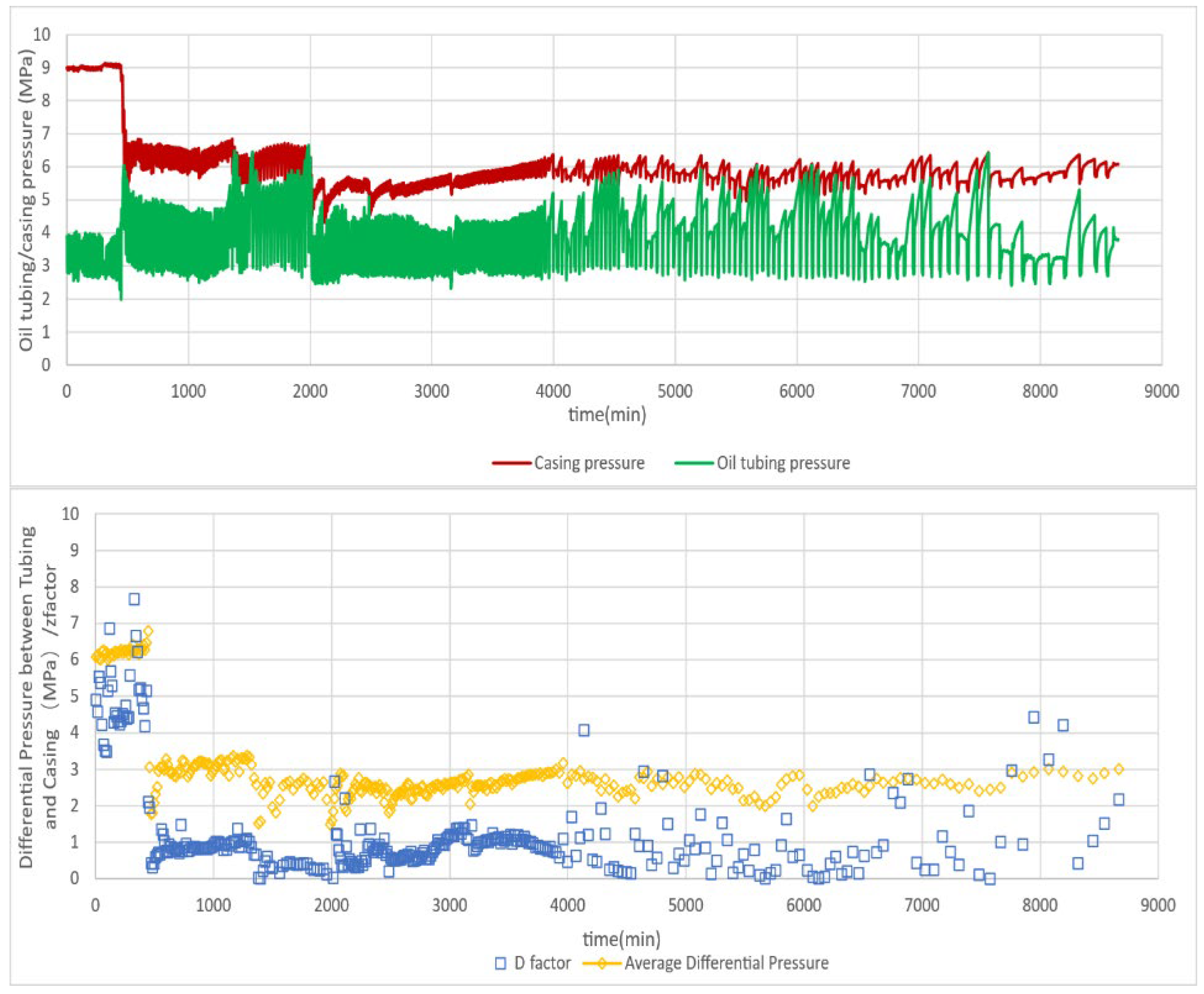
Type I intermittent production wells exhibit stable coefficient D values consistently within the 0.2–0.5 range, with cycle-averaged tubing–casing pressure differential predominantly below 2 MPa. This operational state indicates high liquid unloading efficiency, stable gas–liquid flow regime, timely reservoir energy recharge, and the establishment of a favorable gas-liquid dynamic equilibrium, demonstrating strong stability and high productivity. For example, Well G1 (a representative Type I well) displays the dynamic characteristics shown in
Figure 1. The upper panel illustrates casing pressure/tubing pressure variations over time, while the lower panel presents coefficient D/tubing–casing pressure differential trends. This well maintains a mean coefficient D of 0.35 with a fluctuation range of ±0.08, and cycle-averaged tubing–casing pressure differentials between 1.2 and 1.8 MPa, confirming its classification as a typical Type I intermittent production well.
- (2)
Type II Intermittent Production Wells
Type II intermittent production wells exhibit coefficient D fluctuations within the 0.15–0.75 range, with cycle-averaged tubing–casing pressure differentials around 2 MPa. This operational state reflects relatively high liquid unloading efficiency, stable gas-liquid flow regime, and sufficient reservoir energy recharge, demonstrating robust stability and significant production capacity. For instance, Well G2 (a representative Type II well) displays dynamic characteristics illustrated in
Figure 2. The upper panel shows casing pressure/tubing pressure temporal variations, while the lower panel depicts coefficient D/tubing–casing pressure differential trends. This well maintains a mean coefficient D of 0.45 with fluctuations of ±0.30, and cycle-averaged tubing–casing pressure differentials between 1.6 and 2.2 MPa, confirming its classification as a typical Type II intermittent production well.
- (3)
Type III Intermittent Production Wells
Type III intermittent production wells exhibit coefficient D values approaching zero, with cycle-averaged tubing–casing pressure differentials typically around 1 MPa. This operational state reflects exceptionally high liquid unloading efficiency, stable gas–liquid flow regime, and robust production capacity. The extended closing duration indicates potential for operational parameter optimization. For example, Well G3 (a representative Type III well) demonstrates dynamic characteristics shown in
Figure 3. The upper panel illustrates casing pressure/tubing pressure temporal variations, while the lower panel displays coefficient D/tubing–casing pressure differential trends. This well maintains a mean coefficient D of 0.04 with fluctuations of ±0.13, and cycle-averaged tubing–casing pressure differentials between 0.5 and 1.5 MPa, definitively classifying it as a typical Type III intermittent production well.
- (4)
Type IV Intermittent Production Wells
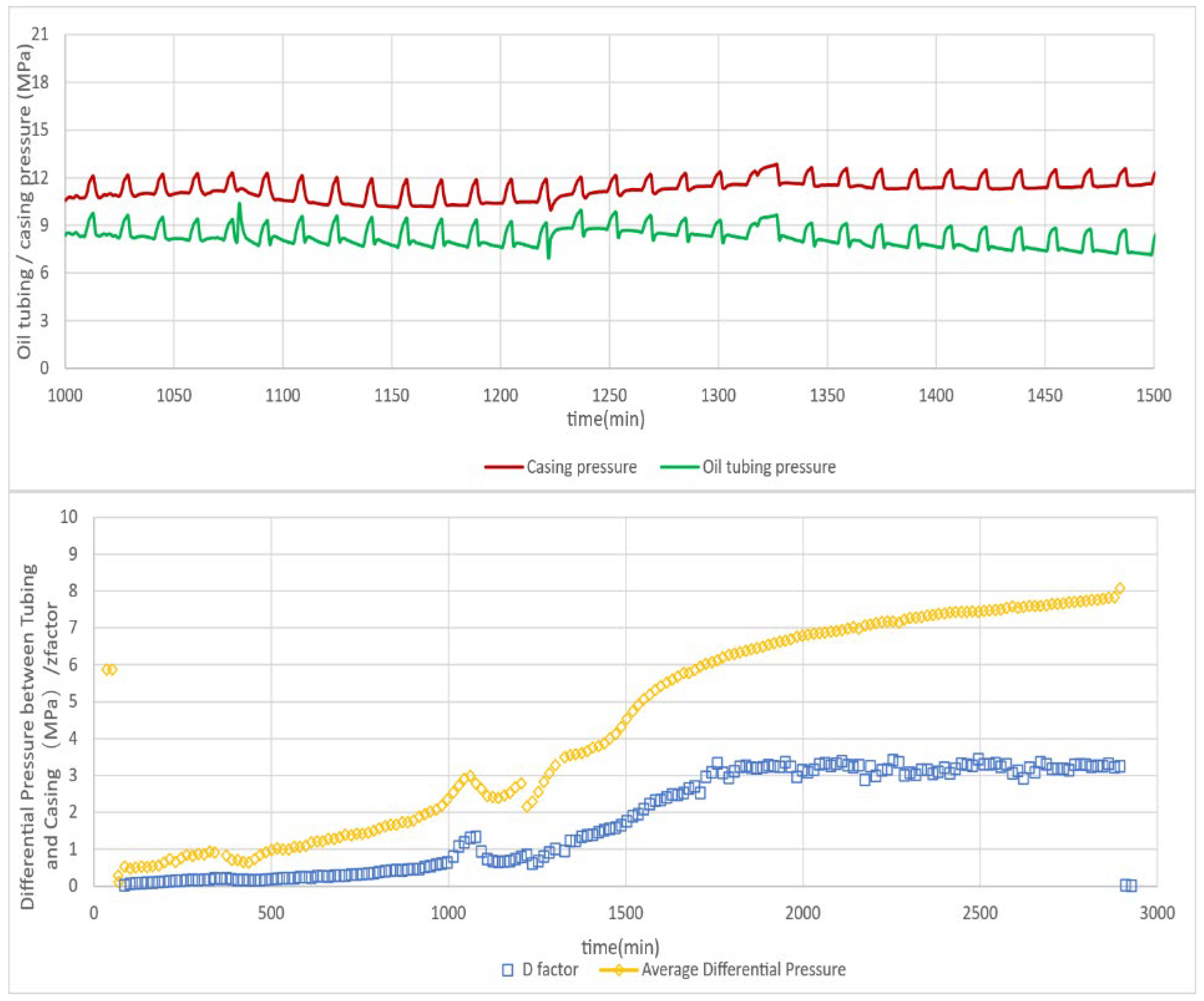
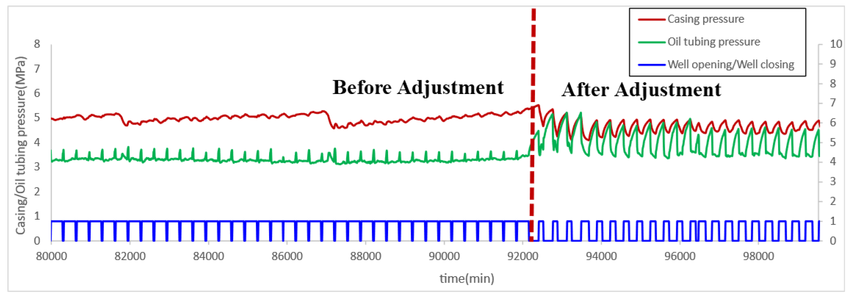
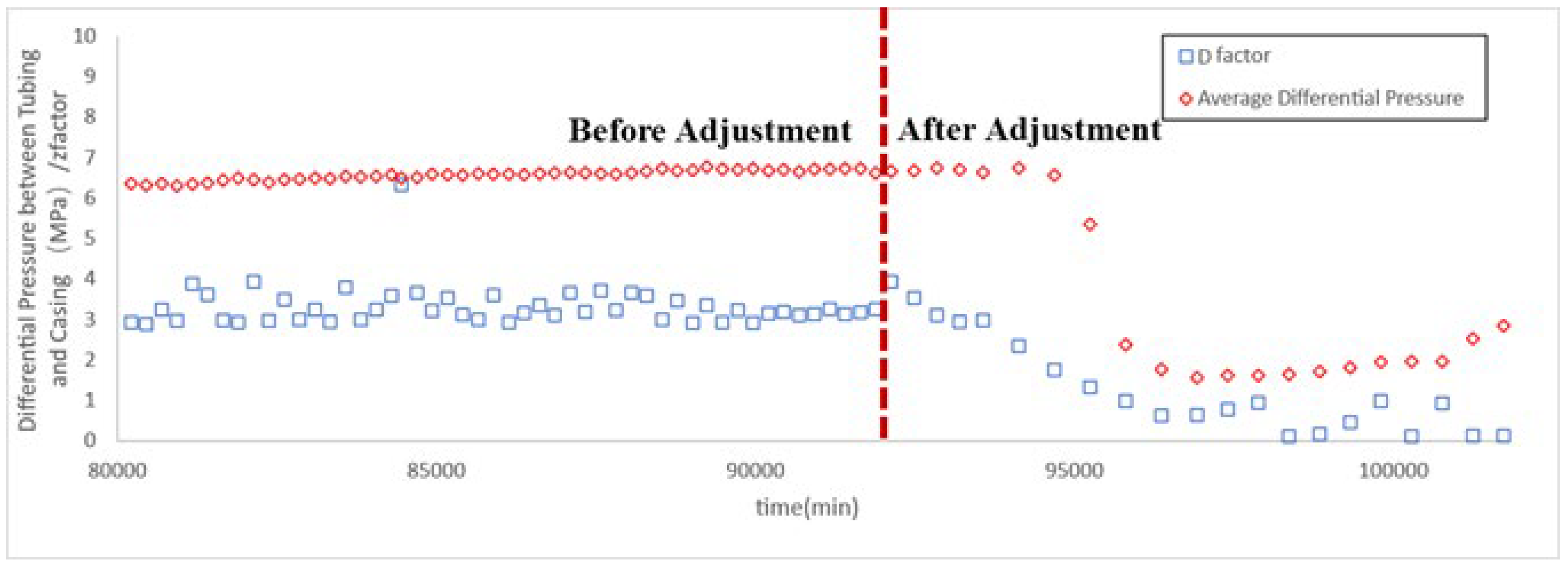
Type IV intermittent production wells exhibit significantly elevated coefficient D values exceeding 3, with cycle-averaged tubing–casing pressure differentials above 5 MPa. This operational state indicates persistent liquid loading in the wellbore, requiring multiple well-opening–closing schedule adjustments to restore normal dynamic equilibrium. For example, Well G4 (a representative Type IV well) demonstrates dynamic characteristics shown in
Figure 4. The upper panel illustrates casing pressure/tubing pressure temporal variations, while the lower panel displays coefficient D/tubing–casing pressure differential trends. After 400 min of operation, through successive schedule adjustments, the well achieved stabilized coefficient D at 0.9 with fluctuations of ±1.1, and cycle-averaged tubing–casing pressure differentials between 2.0 and 3.3 MPa, conclusively identifying it as a typical Type IV intermittent production well.
- (5)
Type V Intermittent Production Wells
Type V intermittent production wells demonstrate a progressive increase in coefficient D from baseline (approaching 0) to elevated levels, accompanied by rising cycle-averaged tubing–casing pressure differentials from 0.5 MPa. This operational state signifies cumulative liquid loading in the wellbore, gradually destabilizing gas-liquid flow regimes, and insufficient reservoir energy recharge, manifesting as deteriorating stability and declining productivity, characteristic of progressive deterioration due to delayed anomaly detection. For instance, Well G5 (a representative Type V well) exhibits dynamic characteristics depicted in
Figure 5. The upper panel shows casing pressure/tubing pressure temporal variations, while the lower panel tracks coefficient D/tubing–casing pressure differential evolution. This well demonstrates coefficient D escalation from 0 to 3.4, with cycle-averaged tubing–casing pressure differentials increasing from 0.5 MPa to 8 MPa, definitively categorizing it as a typical Type V intermittent production well.
- (6)
Type VI Intermittent Production Wells
Type VI intermittent production wells exhibit extreme coefficient D fluctuations (−1 to 2) with cycle-averaged tubing–casing pressure differentials oscillating between 2.5 and 4 MPa. This operational state indicates severe liquid loading, manifested by minimal casing pressure reduction during opening phases and insufficient pressure buildup during closing phases, resulting in attenuated overall CP dynamics. For example, Well G6 (a representative Type VI well) displays dynamic characteristics illustrated in
Figure 6. The upper panel depicts CP/TP temporal variations with constrained amplitude, while the lower panel captures violent coefficient D/tubing–casing pressure differential oscillations. This well demonstrates coefficient D fluctuations spanning −1 to 2, accompanied by cycle-averaged tubing–casing pressure differentials varying between 2.5 and 4 MPa, establishing it as a definitive Type VI intermittent production well.
2.3. Optimization of Well Opening–Closing Durations for Intermittent Production Wells
Based on the classification of intermittent production wells in Jingbian Gas Field and incorporating long-term gas well control experience, this study establishes optimal opening/closing timing for different well types and develops automated switching protocols enabling computer-controlled operations based on real-time tubing pressure, casing pressure, and pipeline pressure variations.
- (1)
Optimization of Opening Duration for Intermittent Production Wells
Analysis of casing pressure dynamics and liquid loading relationships across multiple wells in Jingbian Gas Field reveals that casing pressure buildup during opening phases directly reflects wellbore liquid accumulation. Building upon prior research, we adopt casing pressure buildup as a critical monitoring index for opening duration determination, with field-specific refinements outlined in the operational workflow detailed in
Table 1.
- (2)
Optimization of Shut-in Duration for Intermittent Production Wells
Analysis of opening–closing durations across six well types reveals a strong positive correlation between tubing–casing pressure differentials and coefficient D when average casing pressure during opening phases exceeds 3.5 MPa. Specifically, elevated coefficient D values necessitate extended shut-in durations for pressure recovery, while reduced D values allow shortened shut-in durations to enhance production. To operationalize this relationship, we developed a shut-in duration adjustment methodology using coefficient D as the primary control parameter, with cycle-averaged tubing–casing pressure differentials serving as the performance evaluation metric. The detailed adjustment protocol is presented in
Table 2.
Within the Jingbian Gas Field’s intermittent production well inventory, two special operational scenarios require distinct handling: wells with severely depleted reservoir pressure and those experiencing acute liquid loading.
For wells with critically low reservoir pressure—typically manifested by sustained average casing pressure below 3.5 MPa during opening phases, indicating severely compromised energy reserves—we established a shut-in duration adjustment methodology using opening-phase CP as the primary control parameter. This field-calibrated approach is detailed in
Table 3.
For wells with severe liquid loading, typically manifested by nearly constant tubing–casing pressure differentials throughout both opening and closing phases—exhibiting only transient declines post-opening followed by rapid recovery—effective liquid removal necessitates high-frequency opening operations. Based on field-tested practices, we developed an adjustment strategy focused on shortened opening durations to enhance liquid expulsion efficiency. The detailed protocol is outlined in
Table 4.
To mitigate stochastic and transient operational impacts while complying with Jingbian Gas Field’s mandatory safety thresholds, this methodology employs triple-cycle moving averages of the following parameters as monitoring criteria for systematic adjustments: opening–closing durations, tubing–casing pressure differentials during flow phases, coefficient D, casing pressure buildup, and average casing pressure during production cycles.
Compared to Jingbian Gas Field’s existing optimization approach—which relies solely on casing pressure, empirical casing pressure buildup thresholds, and manual experience—the Coefficient D-based systematic method incorporates more comprehensive factors. It achieves refined well-type classifications, delivers customized optimization schemes while reducing manual workloads and human errors. However, this method requires sufficient historical data collection before implementation due to its data dependency.
3. Research on Staggered Peak-Shifting Group Control Methodology for Multiple Wells in Jingbian Gas Field
3.1. Data Acquisition and Preprocessing
Intermittent production wells in Jingbian Gas Field exhibit high initial gas rates during opening phases, making simultaneous activation of multiple wells prone to cause significant pressure and flowrate fluctuations at gas gathering stations, thereby compromising compressor and dehydration skid operations. This necessitates the development of a staggered peak-shifting group control algorithm that coordinates well activation timing while maintaining optimal productivity. The staggered control methodology requires historical production data from individual wells to precisely predict peak-shifting windows, including: production timeline, well status (open/closed), current cycle shut-in duration, current cycle opening duration, elapsed time in current cycle, pipeline pressure, tubing pressure, and casing pressure. The absence of wellhead flow meters precludes the acquisition of instantaneous/cumulative flowrates. Given the dynamic switching status across the well population, the algorithm must prioritize real-time capability through continuous acquisition of system timestamps, well statuses, instantaneous flowrates (if available), and pressure data, ensuring time-sensitive optimization. This study established a dedicated database extracting critical parameters from Jingbian Gas Field’s existing data network platform, with a data polling interval of 10 min. Automated analysis of this dataset enables the derivation of cycle-specific parameters for each intermittent producer.
After confirming data sources and obtaining relevant permissions, real-time data is retrieved via an HTTP connection to the remote TDengine database on the centralized acquisition platform. For data preprocessing, standardized normalization and categorized anomaly handling address data inconsistencies including non-uniform storage formats across Jingbian Gas Field operational areas and abnormal intermittent well behaviors; specifically: production data for individual wells is extracted from separate well tables, and to maintain consistency, all source database time-series data is uniformly collected as analytical inputs. For anomaly processing, 72 h of historical data is secured as the analysis baseline to exclude non-cycled wells (permanently shut-in or flowing). Outliers in production data (e.g., well status “−3” or zero-value sequences) trigger well-level anomaly classification when exceeding a 15% threshold. Additionally, tiered communication failure protocols are implemented: (1) Wells offline for >4 h are treated as anomalies due to real-time data loss and control failure; (2) Wells with >70% missing historical data are classified as communication–failure anomalies.
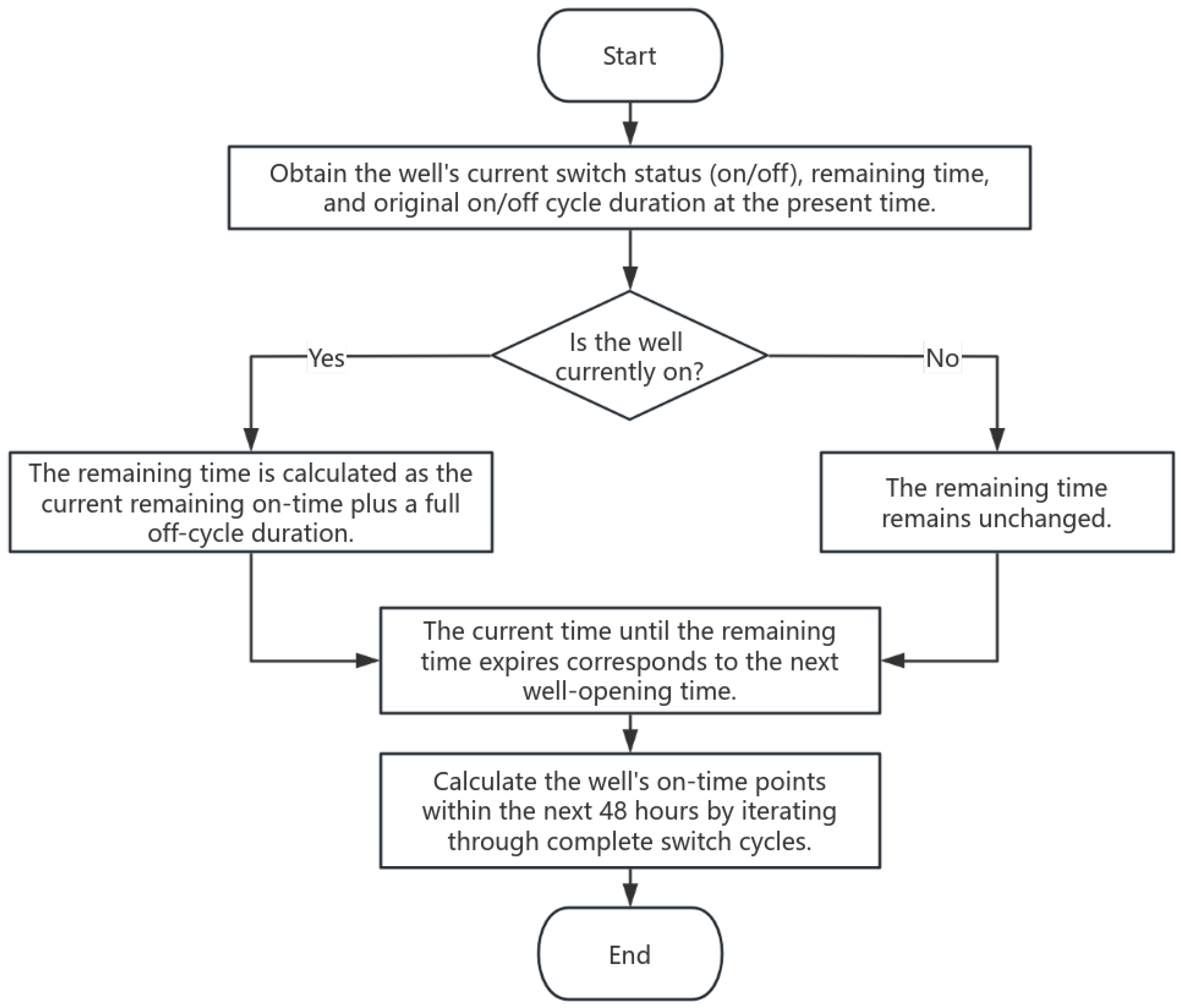
3.2. Well Opening Time Prediction
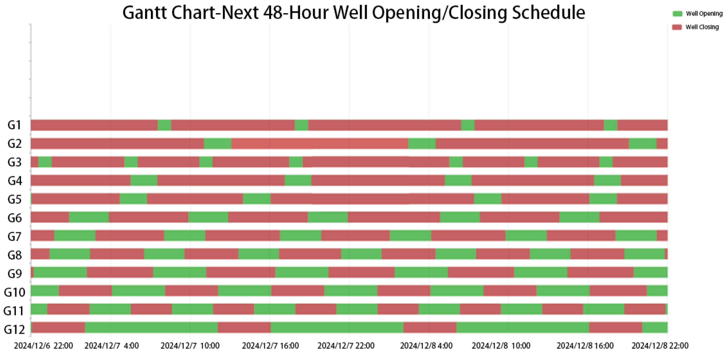
When multiple wells exhibit overlapping opening schedules, the control system prioritizes deferral of low-productivity wells while minimizing production loss through constrained extension of individual well shut-in durations. Prior to implementing staggered optimization, 48 h opening time predictions must be generated for each intermittent producer. For every well, the prediction algorithm calculates prospective opening windows within the 48 h horizon based on current status (open/closed), active cycle durations (opening/shut-in), and remaining phase time. This workflow, detailed in
Figure 7, generates time-staggered activation schedules that balance peak shaving with production optimization.
During field implementation, discrepancies between recorded and actual opening–closing durations may arise due to network latency in well clusters and valve actuation rate inconsistencies. These errors have been systematically incorporated into our error compensation framework through algorithmic adjustments and real-time calibration protocols within Jingbian Gas Field’s data network platform.
3.3. Staggered Peak-Shifting Group Control Methodology
Simultaneous activation of multiple wells induces pressure and flow rate fluctuations at gas gathering stations. Therefore, well clusters and timestamps generating such peaks are identified as conflict peaks requiring resolution. The control protocol prioritizes deferring low-productivity wells’ opening operations while minimizing shut-in duration extensions to mitigate production impacts.
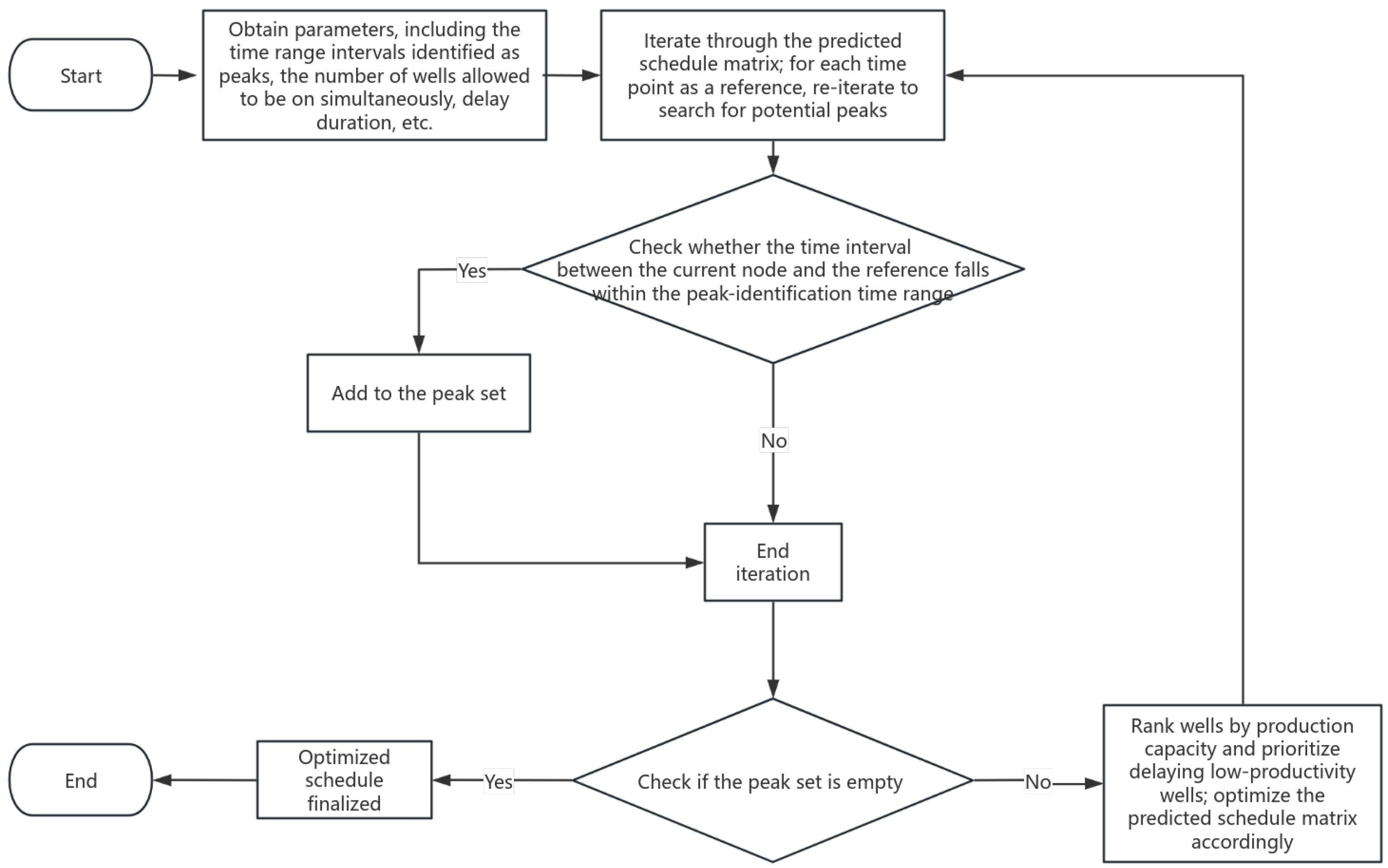
The staggered peak-shifting group control algorithm requires three critical input parameters: (1) Peak Identification Time Window, defined as the maximum allowable time overlap for concurrent well openings among multiple wells; (2) Maximum Simultaneous Opening Capacity, specifying the permitted number of parallel-activated wells; and (3) Deferred Opening Interval, referring to the mandatory time delay imposed on low-productivity wells when resolving multi-well peak conflicts. The Peak Identification Time Window quantifies the temporal tolerance for synchronized operations, while the Deferred Opening Interval establishes prioritized displacement durations based on well productivity hierarchies.
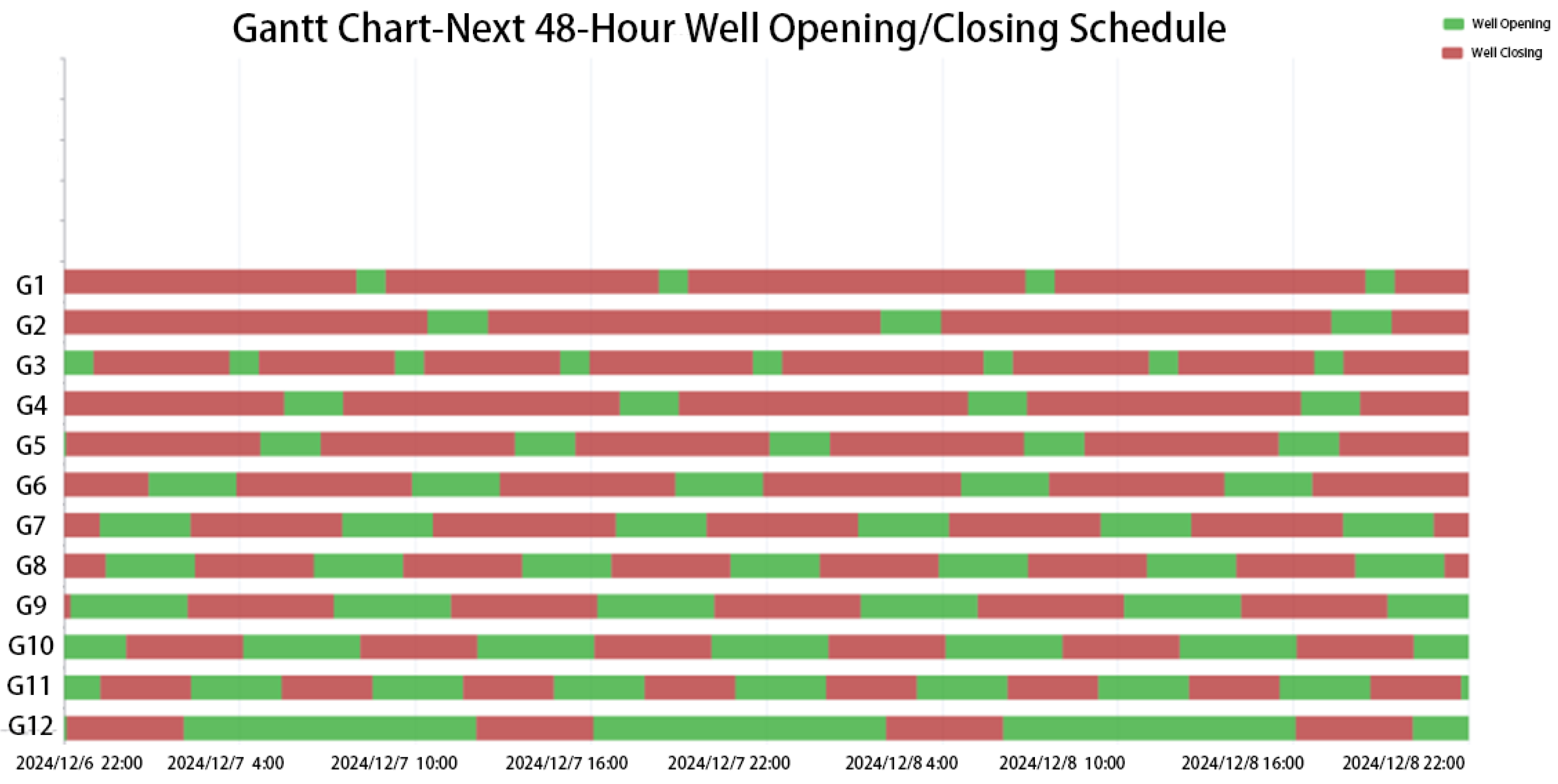
This study employs an exhaustive enumeration method, systematically iterating through predicted opening schedules to detect and resolve all conflict peaks via temporal displacement. The workflow, as detailed in
Figure 8, achieves complete peak elimination through predictive traversal and adaptive rescheduling.
The algorithmic framework initiates by predetermining prospective opening times for all intermittent production wells. Through systematic traversal of each well, those exceeding the Peak Identification Time Window threshold are aggregated into conflict peak sets. This process culminates in a finalized conflict peak set requiring resolution, where each set represents temporally overlapping operations within a defined window.
All wells are prioritized based on measured productivity rankings from Jingbian Gas Field’s single-well tests. During peak resolution, low-productivity wells undergo prioritized deferral with real-time updates to their opening schedules. The algorithm iteratively regenerates updated peak sets until complete elimination is achieved.
Assuming a 15 min Peak Identification Time Window, two operational scenarios are evaluated: ① Centered Window: ±15 min around a well’s scheduled opening time triggers peak identification. ② Forward Window: Only subsequent 15 min intervals post-opening are monitored. Empirical testing demonstrates that Scenario ① introduces false positives by overextending detection ranges, whereas Scenario ② enables precise peak elimination through controlled iterations.
After extensive trials, the deferred opening interval resolution achieves 1 min iteration precision. Post-deferral wells automatically revert to their original intermittent production schedules in subsequent cycles. The optimized staggered control parameters are then exported for field implementation.


