Application of the NOA-Optimized Random Forest Algorithm to Fluid Identification—Low-Porosity and Low-Permeability Reservoirs

Abstract

As an important unconventional oil and gas resource, tight oil exploration and development is of great significance to ensure energy supply under the background of continuous growth of global energy demand. Low-porosity and low-permeability reservoirs are characterized by tight rock properties, poor physical properties, and complex pore structure, and as a result the fine calculation of logging reservoir parameters faces great challenges. In addition, the crude oil in this area has high viscosity, the formation water salinity is low, and the oil reservoir resistivity shows significant spatial variability in the horizontal direction, which further increases the difficulty of oil and water reservoir identification and affects the accuracy of oil saturation calculation. Targeting the above problems, the Nutcracker Optimization Algorithm (NOA) was used to optimize the hyperparameters of the random forest classification model, and then the optimal hyperparameters were input into the random forest model, and the conventional logging curve and oil test data were combined to identify and classify the reservoir fluids, with the final accuracy reaching 94.92%. Compared with the traditional Hingle map intersection method, the accuracy of this method is improved by 14.92%, which verifies the reliability of the model for fluid identification of low-porosity and low-permeability reservoirs in the research block and provides reference significance for the next oil test and production test layer in this block.

1. Introduction

With the rapid expansion of the global economy and the continuous improvement of exploration technology, as well as the sustained growth in demand for oil and gas resources, the proportion of low-porosity and low-permeability oil and gas reservoirs in China’s oil and gas production has been increasing year by year. The importance of these reservoirs is becoming increasingly prominent, and they are gradually becoming a key area for oil and gas exploration and development in China. It is expected that low-porosity and low-permeability oil and gas resources will become the mainstream of China’s oil and gas resources in the future [1].

Currently, the reserves of oil and gas reservoirs with low porosity and low permeability account for nearly 70% of the domestically proven oil and gas reserves, making them the core targets for exploration and development [1]. In the process of exploring and developing oil and gas fields, the identification of fluid properties in low-porosity and low-permeability reservoirs is one of the key steps, and its accuracy directly determines the effective discovery and efficient development of oil and gas layers. In low-porosity and low-permeability reservoirs, improving the accuracy of fluid property identification is of significant importance. Compared to conventional reservoirs, these reservoirs exhibit more complex rock pore structures, higher physical heterogeneity, and irregular distributions of oil, gas, and water, leading to complex and variable logging responses [2]. Due to the lower porosity, the fluid content in the reservoir is also relatively low, causing the lithologic contribution to logging electrical responses to be much greater than that of fluids [3]. As a result, the differences in logging curves between oil layers, gas layers, oil–water mixed layers, water layers, and dry layers are not obvious. Therefore, relying solely on logging data for fluid property identification poses significant challenges [4].

This paper proposes to combine the Nutcracker Optimization Algorithm (NOA for short) with the random forest classification model for reservoir fluid identification. The Nutcracker Optimization Algorithm, introduced by Mohamed Abdel-Basset et al. in 2023 [5], is a bio-inspired optimization algorithm based on the foraging, caching, and food retrieval behaviors of nutcrackers. By simulating the foraging behavior of nutcrackers, NOA can effectively perform a global search across the entire parameter space, which helps to avoid local optima and increases the probability of finding the global optimal combination of hyperparameters. Additionally, the accuracy of this method will be compared with that of the traditional Hingle intersection method to evaluate its applicability in the local region.

2. Research Background

The structural position of this oilfield is influenced by the dual control of the Altun Fault and the Kunbei strike-slip fault, with both structural evolution and sedimentary characteristics being affected by the activities of these faults [6]. In the study area, three major provenance systems developed during the Cenozoic sedimentary period: the northwest provenance system provided a stable supply of coarse clastic sediments from a proximal source; although more distant, the southwest provenance system offered a consistent supply of mixed sediments ranging from coarse to fine grains; conversely, the northeast provenance system exhibited an unstable supply and was relatively far away, primarily transporting coarse clastic materials. These provenance characteristics directly governed the distribution patterns of sedimentary facies belts: alluvial fans and nearshore submarine fans predominantly developed in the northwest and northeast source areas, while braided deltas were concentrated in southern regions [7,8]. Additionally, lacustrine and shallow lacustrine facies were distributed between fan bodies and in eastern areas. Research indicates that during the Cenozoic sedimentary period, the scale of development for each facies belt was closely correlated with source supply intensity—when source supply was abundant, not only did the thickness of nearshore submarine fans significantly increase, but their leading edges also extended further into lake basin centers, resulting in a corresponding reduction in the extent of lacustrine and shallow lacustrine facies belts [9].

Through the analysis of core rock samples from nine wells in the block (as shown in

Table 1. Statistical data of rock sample analysis.

Well Number	Core Analysis Porosity		Core Analysis Permeability
	Range (%)	Average (%)	Range (mD)	Average (mD)
33	7.0~11.0	9.52	0.100~147.100	6.740
31	9.7~12.0	10.73	0.031~112.600	6.290
26	5.4~11.4	9.59	0.004~255.200	6.279
36	6.5~11.9	9.54	0.002~29.500	1.595
12	7.0~11.1	9.71	0.033~128.698	3.293
5	6.0~16.3	12.57	0.010~156.170	6.544
3	10.2~15.5	14.51	0.103~27.976	3.749
21	7.0~13.4	10.07	0.100~78.400	7.721
14	6.1~13.1	9.44	0.002~147.61	5.239

), the porosity of the target zone in the study area is mainly distributed between 6.1 and 16.3%, with an average of 10.63%. The permeability mainly ranges from 0.002 to 255.200 mD, with an average of 5.272 mD, which is classified as a low-porosity and low-permeability reservoir; the reservoir lithology is mainly fine sandstone and silty fine sandstone, with minor amounts of fine sandstone, coarse sandstone, and conglomerate. The oil content is primarily fluorescence, oil traces, and oil stains, with fewer oil-soaked and oil-rich occurrences.

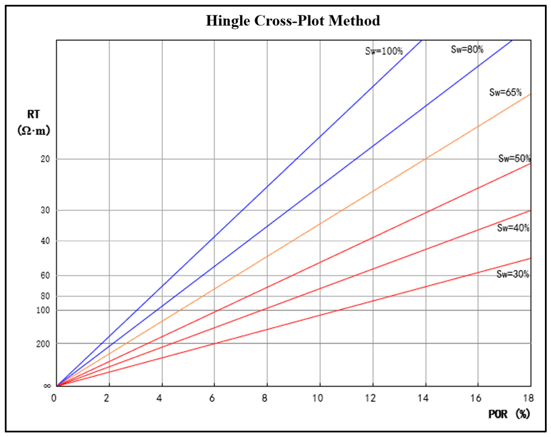
3. Hingle Cross-Plot Method

3.1. Principle

The Hingle cross-plot method is based on Archie’s formula (Equation (1)):

$$S_w=\sqrt[n]{{\displaystyle \frac{a\times b\times R_w}{{\varphi }^m\times R_t}}}$$

(1)

In the formula, $S_w$ represents the water saturation (as a decimal), a is the rock property coefficient related to lithology, b is a constant related to rock properties, n is the saturation exponent, m is the cementation exponent, $R_w$ is the formation water resistivity (Ω·m), $R_t$ is the measured formation resistivity (Ω·m), and ϕ is the porosity (as a decimal).

Equation (1) can be transformed into Equation (2):

$${\displaystyle \frac{1}{\sqrt[m]{R_t}}}=\sqrt[m]{{\displaystyle \frac{S_w^n}{a\times b\times R_w}}}\times \varphi$$

(2)

The values of a, b, m, and n vary depending on the region and can be obtained through the analysis of rock electrical experiments; the formation water resistivity $R_w$ can be determined from water analysis data or calculated based on well logging data by identifying pure water layers. For a specific block, $R_w$ can be a constant value. Therefore, within a certain interpretation interval and for a determined water saturation $S_w$, we can set $\sqrt[m]{S_w^n/\left(a\times b\times R_w\right)}=A$ (where A is a constant). By constructing the y-axis with the scale $1/\sqrt[m]{R_t}$ and the x-axis with a linear scale $x=\varphi$, Equation (2) becomes the linear equation $y=Ax$ on the $1/\sqrt[m]{R_t}-\varphi$ cross-plot, and this line passes through the origin ($\varphi$ = 0, $R_t=\infty$). Different lines can be obtained based on various $S_w$ values, leading to the construction of a resistivity–porosity cross-plot scaled by $S_w$, which is known as the Hingle cross-plot (as shown in Figure 1) [10].

3.2. Nutcracker Optimization Algorithm (NOA)

The Nutcracker Optimization Algorithm (NOA), proposed by Mohamed Abdel-Basset and others in 2023 [5], is a bio-inspired optimization algorithm based on the foraging behavior of the Clark’s nutcracker. The behavior of the nutcracker primarily consists of two parts: the first part involves collecting and storing food, while the second part involves searching for and retrieving the stored food. These two behaviors occur in distinct periods. The first behavior takes place in summer and autumn, while the second behavior occurs in winter and spring. NOA formulates its algorithmic strategies based on the above two behaviors, with the two main strategies being (1) foraging and caching strategy, and (2) cache searching and retrieval strategy. Similar to other population-based optimization algorithms, the population initialization in NOA is performed using Equation (3).

$${\overrightarrow{X}}_{i,j}^t=\left({\overrightarrow{U}}_j-{\overrightarrow{L}}_j\right)\times \overrightarrow{RM}+{\overrightarrow{L}}_j, i=1,2,\dots ,N, j=1,2,\dots ,D$$

(3)

In the formula, ${\overrightarrow{X}}_{i,j}^t$ represents the j-th position of the i-th generation of nutcrackers, U_j is the upper bound of the optimization parameter, L_j is the lower bound of the optimization parameter, and RM is a random number in the interval [0, 1], ensuring that the initial positions are uniformly distributed within the search space.

First is the foraging and storage strategy, which involves two phases: exploration and exploitation. The exploration phase is represented by Equation (4), while the exploitation phase is described by Equation (5). Furthermore, the balance between exploration and exploitation is maintained through Equation (6) [5,11,12].

$${\overrightarrow{X}}_i^{t+1}=\left\{\begin{array}{c}{X}_{i,j}^t if \tau 1<\tau 2\\ \left\{\begin{array}{c}{X}_{m,j}^t+\gamma \left(X_{A,j}^t-X_{B,j}^t\right)+\mu \left(r^2{U}_j-L_j\right),if \tau <{\displaystyle \frac{T_{max}}{2}}\\ X_{C,j}^t+\mu \left(X_{A,j}^t-X_{B,j}^t\right)+\mu \left(r1<\delta \right)\left(r^2{U}_j-L_j\right),Otherwise\end{array}Otherwise\right.\end{array}\right.$$

(4)

In the formula, X_i^t+1 is the new position of the i-th nutcracker in the t-th iteration; X^t_i,j is the j-th position of the i-th nutcracker in the current generation; γ is a random number generated based on the Lévy flight; X^t_best,j is the best solution obtained so far in the j-th dimension; A, C, and B are three different indices randomly selected from the population to promote the exploration of high-quality “food” sources; τ1, τ2, r, and r1 are random real numbers within the range [0, 1]; X^t_m,j is the mean of all solutions in the j-th dimension of the population in the t-th generation; and μ is a value generated based on a normal distribution (τ4), Lévy flight (τ5), and a random number between (0, 1) (τ3) [11], as shown in Equation (5).

$${\overrightarrow{X}}_i^{t+1\left(new\right)}=\left\{\begin{array}{c}{\overrightarrow{X}}_i^t+\mu \left({\overrightarrow{X}}_{best}^t-{\overrightarrow{X}}_i^t\right)\left|\lambda \right|+r1\left({\overrightarrow{X}}_A^t-{\overrightarrow{X}}_B^t\right), if \tau 1<\tau 2\\ {\overrightarrow{X}}_{best}^t+\mu \left({\overrightarrow{X}}_A^t-{\overrightarrow{X}}_B^t\right) , if \tau 1<\tau 3\\ {\overrightarrow{X}}_{best}^{t}l , Otherwise\end{array}\right.$$

(5)

In the formula, X_i^t+1(new) represents the new position of the i-th nutcracker in the t-th iteration, λ is a random number generated according to the Lévy flight distribution, τ3 is a random number between 0 and 1, and l is a linearly decreasing factor from 1 to 0, introduced to enhance diversity in the exploitation behavior of NOA. This factor helps to avoid local minima that may occur during search in a particular direction and accelerates the convergence of the algorithm.

$$\mu =\left\{\begin{array}{c}\tau 3, if r1<r2\\ \tau 4, if r2<r3\\ \tau 5, if r1<r3\end{array}\right.$$

(6)

In the formula, r2 and r3 are random real numbers within the range [0, 1].

In addition, the exploration and exploitation phases maintain a balance between them by the following equation.

$${\overrightarrow{X}}_i^{t+1}=\left\{\begin{array}{c}Equation \left(4\right), if \phi >P_{a1}\\ Equation \left(5\right), Otherwise\end{array}\right.$$

(7)

In the formula, φ is a random number between (1, 0), and P_a1 is the probability value that linearly decreases from 1 to 0 based on the current generation number.

Secondly, the search and retrieval strategy for caches also goes through two phases: exploration and exploitation. However, the cache search strategy is primarily based on the exploration and exploitation of caches. The search process is shown in Equations (8) and (9). The difference between the exploration and exploitation processes lies in the selection of different caching strategies, which are detailed in Equations (10) and (11). Similar to the first strategy, the balance between exploration and exploitation is maintained through a formula [5,11,12], as seen in Equation (12).

$${\overrightarrow{RP}}_{i,1}^t=\left\{\begin{array}{c}{\overrightarrow{X}}_i^t+\alpha \cos \left(\theta \right)\left(\left({\overrightarrow{X}}_A^t-{\overrightarrow{X}}_B^t\right)\right)+\alpha RP, if \theta ={\displaystyle \frac{\pi }{2}}\\ {\overrightarrow{X}}_i^t+\alpha \cos \left(\theta \right)\left(\left({\overrightarrow{X}}_A^t-{\overrightarrow{X}}_B^t\right)\right), Otherwise\end{array}\right.$$

(8)

$${\overrightarrow{RP}}_{i,2}^t=\left\{\begin{array}{c}{\overrightarrow{X}}_i^t+\left(\alpha \cos \left(\theta \right)\left(\left(\overrightarrow{U}-\overrightarrow{L}\right)\tau 3+\overrightarrow{L}\right)+\alpha RP\right)\overrightarrow{U_2}, if \theta ={\displaystyle \frac{\pi }{2}}\\ {\overrightarrow{X}}_i^t+\alpha \cos \left(\theta \right)\left(\left(\overrightarrow{U}-\overrightarrow{L}\right)\tau 3+\overrightarrow{L}\right)\overrightarrow{U_2}, Otherwise\end{array}\right.$$

(9)

In the formula, ${\overrightarrow{RP}}_{i,1}^t$ and ${\overrightarrow{RP}}_{i,2}^t$ represent the cache positions of the i-th Clark’s nutcracker during the t-th iteration, Xit denotes the cache of the i-th Clark’s nutcracker at the t-th iteration on the current day, α linearly decreases from 1 to 0, $\overrightarrow{r2}$ is a vector of random values within the range [0, 1], τ3 is a random number within the range [0, 1], θ is a random number within the range [0, π], and Prp represents the probability used to determine the proportion of global exploration in the search space.

$$X_{i,j}^{t+1}=\left\{\begin{array}{c}{X}_{i,j}^t, if \tau 3<\tau 4\\ X_{i,j}^t+r1\left(X_{best,j}^t-X_{i,j}^t\right)+r2\left({\overrightarrow{RP}}_{i,1}^t-X_{C,j}^t\right), Otherwise\end{array}\right.$$

(10)

$$X_{i,j}^{t+1}=\left\{\begin{array}{c}{X}_{i,j}^t, if \tau 5<\tau 6\\ X_{i,j}^t+r1\left(X_{best,j}^t-X_{i,j}^t\right)+r2\left({\overrightarrow{RP}}_{i,2}^t-X_{C,j}^t\right),Otherwise\end{array}\right.$$

(11)

$${\overrightarrow{X}}_i^{t+1}=\left\{\begin{array}{c}Equation \left(10\right), if \phi >P_{a2}\\ Equation \left(11\right), Otherwise\end{array}\right.$$

(12)

In the formula, ${\overrightarrow{X}}_i^{t+1}$ represents the new position or cache of the i-th Clark’s nutcracker during the (t + 1)-th iteration, and C is the index of a solution randomly selected from the population.

Through the above elaboration, NOA demonstrates its global exploration capability and dynamic adjustment of the search process in foraging and storage strategies. By simulating the foraging behavior of Clark’s nutcracker in nature, the algorithm employs Lévy flight and a random number generation mechanism to conduct effective global searches in vast search spaces, thereby increasing the likelihood of discovering the global optimum. Meanwhile, the algorithm achieves a dynamic balance between exploration and exploitation phases, enabling it to maintain sufficient diversity while conducting more detailed searches in promising areas. This balancing strategy not only avoids premature convergence to local optima but also accelerates the convergence rate, enhancing search efficiency. Secondly, NOA further demonstrates its memory-based search advantages and flexible search strategies in the context of storage item search and retrieval. The algorithm memorizes previously found high-quality solutions and uses them as reference points in the search process, effectively leveraging historical information to guide the current search direction. Additionally, the probabilistic control mechanism within the algorithm enables global exploration, enhancing the likelihood of locating the global optimum. This flexible mechanism, which combines stochastic and deterministic characteristics, allows the algorithm to adapt to a wide range of complex optimization problems, ensuring efficient search in terms of both the breadth and depth of the solution space [5,12,13].

4. Data Processing and Result Analysis

4.1. Hingle Intersection Diagram Method

Based on the electrical classification, according to the thickness of the reservoir, physical properties, oil bearing, and other parameters, and combined with the oil test conclusion (wells with a return rate greater than 100%, as shown in

Table 2. Oil test conclusions of wells with back-flushing rates greater than 100%.

Test Zone Number	Oil Test Conclusion	Test Zone Number	Oil Test Conclusion
1	Oil–water coexistence layer	18	Oil–water coexistence layer
2	Oil–water coexistence layer	19	Oil–water coexistence layer
3	Oil–water coexistence layer	20	Oil–water coexistence layer
4	Oil-bearing layer	21	Oil–water coexistence layer
5	Oil-bearing layer	22	Oil–water coexistence layer
6	Oil-bearing layer	23	Oil–water coexistence layer
7	Oil-bearing layer	24	Oil–water coexistence layer
8	Oil-bearing layer	32	Oil–water coexistence layer
10	Oil-bearing layer	33	Oil–water coexistence layer
14	Oil–water coexistence layer	34	Oil-bearing layer
15	Oil–water coexistence layer	35	Oil–water coexistence layer
16	Oil–water coexistence layer	36	Oil–water coexistence layer
17	Oil–water coexistence layer

), it is divided into five categories: oil layer, oil–water layer, oil-bearing water layer, water layer, and dry layer, and the specific classification criteria are shown in

Table 3. Identification criteria for effective layer fluids.

Fluid Type	Porosity/%	Oil Saturation/%
Oil-bearing layer	≥12	≥58
Oil–water coexistence layer	≥8	≥35
Oil-bearing water layer	≥8	≥10
Water layer	>8	<10
Dry layer	<8	/

. Based on this, the oil and water layer identification chart of the Hingle intersection method (Figure 2) was established, and the fluid identification accuracy rate was 80% (No. 5, No. 6, No. 7, No. 8, and No. 36 oil test layers could not be accurately identified on the chart), which could better identify different fluid types and was suitable for this research block. The cause of the low-resistance reservoir [14,15] needs further research and verification and is not within the scope of this paper.

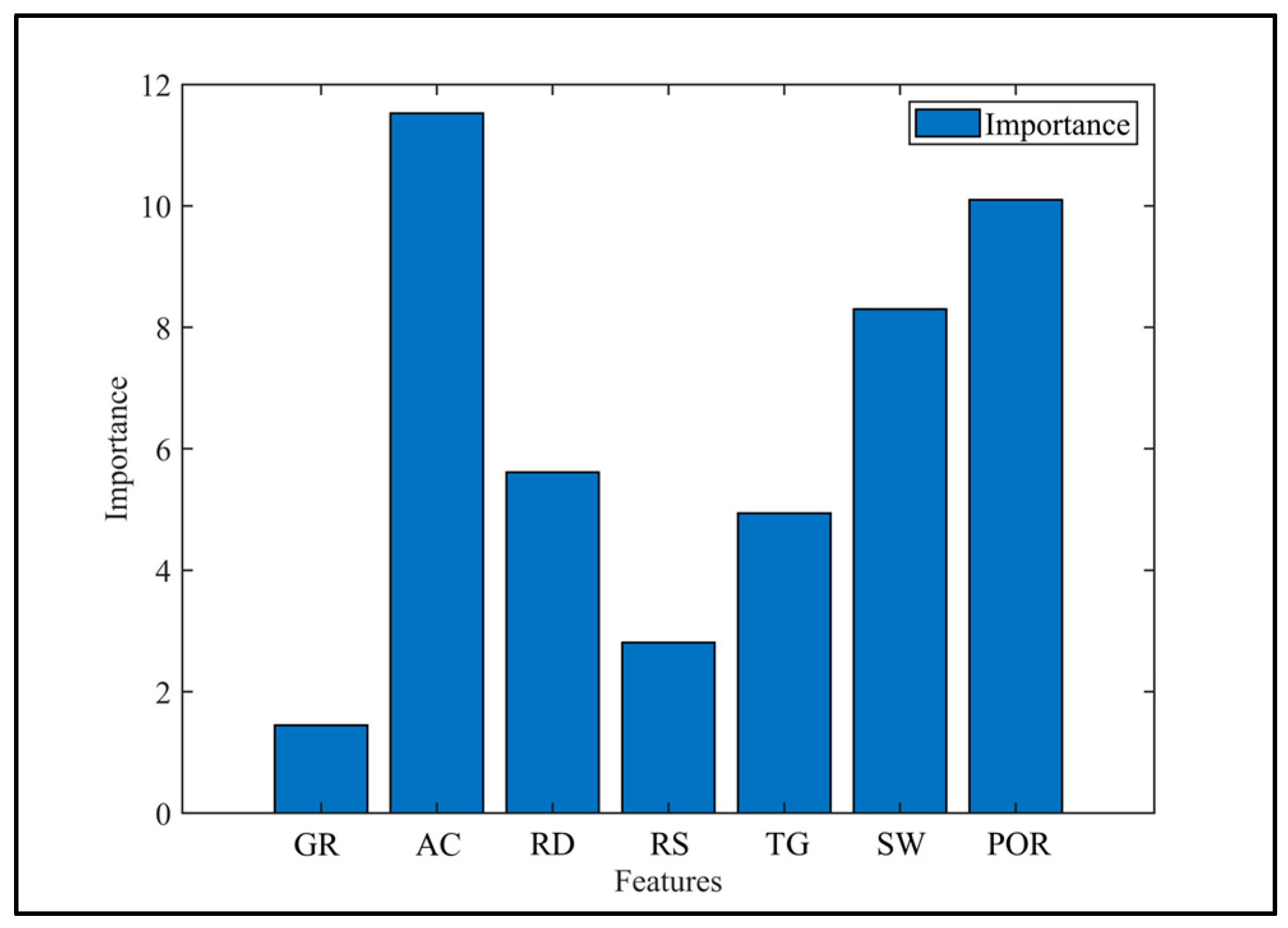
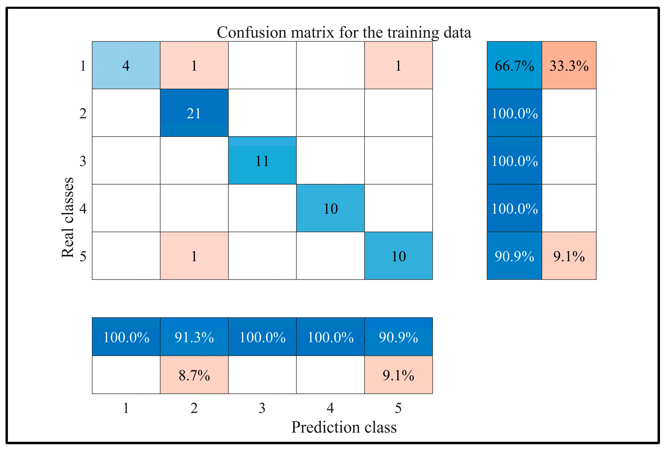
4.2. NOA-Optimized Random Forest Classification Method

Random forest is a classic classification algorithm based on the ensemble learning framework. It significantly enhances the generalization performance and robustness of the model by constructing multiple decision trees and integrating individual prediction results. This algorithm was proposed by Leo Breiman in 2001, and its core mechanism features double randomness. Firstly, multiple sub-training sets are generated from the original dataset through bootstrap sampling. Each subset is used to train an independent decision tree, which ensures diversity at the data level. Secondly, during the node-splitting process of each tree, only a specific number of feature subsets are randomly selected from all features to choose the splitting attributes, further introducing randomness at the feature level. Each decision tree follows a full-growth strategy until the node purity reaches the preset threshold. Finally, the prediction results of all trees are aggregated through the majority-voting mechanism [16].

Before applying the random forest algorithm for classification, it is necessary to normalize the data to eliminate the impact of scale differences among different variables. The logging curve data, which serves as feature values, should be normalized according to Formula (13), ensuring that all variable values are mapped to the interval [0, 1]. This process guarantees that during the training phase, each feature value is comparable and consistent, thereby enhancing the accuracy and reliability of the classification.

$$x_i^{\prime }={\displaystyle \frac{x_i-x_{min}}{x_{max}-x_{min}}}\left(i=1,2,3\dots m\right)$$

(13)

In the formula, $x_i^{’}$ represents the normalized value, $x_i$ represents the original value of the sample, $x_{min}$ represents the minimum original value of the sample, $x_{max}$ represents the maximum original value of the sample, and m represents the number of samples. As shown in Figure 3, in the MATLAB (Version 2019a) environment, when the population size of the NOA-optimized random forest is set to 30 (population size refers to the total number of individuals searched in parallel in each iteration of the algorithm) and the number of iterations approaches 300, the results stabilize. Therefore, it is sufficient to set the number of iterations to 300.

As shown in

Table 4. Random forest parameter table.

Model Parameters	Optimization Range	Optimal Value
ntree	10~500	10 (10.0)
mtry	1~10	6 (6.4098)

, hyperparameter optimization is conducted for two modeling parameters of the random forest model [16,17]. These parameters are the number of trees in the forest (ntree), which represents the total number of decision trees included in the algorithm, and the decision tree depth (mtry), which refers to the number of nodes on the longest path of the tree and is also the length of the node path from the root node to the farthest leaf. The upper and lower bounds of the optimization ranges for the above two parameters are stored in arrays U and L, respectively, and then input into the Nutcracker Optimization Algorithm (NOA) to find the optimal values. In NOA, the five-fold cross-validation method is specifically used as a reference to evaluate the model effect of each iteration, and this method is employed to search for the optimal values in the parameter space [18,19,20,21]. Five-fold cross-validation means that during each iteration, the dataset is randomly divided into five sub-sample sets of equal size. Each time, one of the sub-sample sets is selected as the test set, and the remaining four sub-sample sets are used as the training set. Through five iterations, it is ensured that each sub-sample set is used as the test set once [22]. In this study, the gamma ray curve (GR), acoustic transit time curve (AC), deep resistivity curve (RD), shallow resistivity curve (RS), total hydrocarbon curve (TG), calculated water saturation curve (SW), and calculated porosity curve (POR), which are available in most wells, are selected as the input feature curves. The GR curve mainly reflects the shale content of the reservoir. The AC curve and POR curve mainly reflect the storage capacity of the reservoir. The RD curve, RS curve, and SW curve mainly reflect the oil-bearing property of the reservoir. The difference between the RD curve and the RS curve can, to a certain extent, reflect the seepage capacity of the reservoir. The TG curve can qualitatively determine the oil-bearing property of the reservoir. The sample data is divided into a training set (a dataset used for training the machine learning model) and a test set (a dataset used for evaluating the model performance) at a ratio of 7:3. Figure 4 shows the weight values of each curve in the trained model. (The testing hardware is a laptop computer: CPU: 13th Gen Intel(R) Core(TM) i9-13900HX; GPU: NVIDIA GeForce RTX 4060 Laptop (Equipment purchased from Yuncheng City, Shanxi Province, China, manufacturer Lenovo); RAM: two DDR5-8GB memory modules. The operating environment is MATLAB (Version 2019a) software, and the running time is 482 s.)

According to the confusion matrix of the training set shown in Figure 5 (a confusion matrix is an N × N matrix that shows the correspondence between the model’s prediction results and the true labels; the diagonal elements represent correct classifications, while the off-diagonal elements represent misclassification cases, providing a quantitative basis for model optimization), the accuracy of the random forest model optimized by NOA in the classification task reaches 94.92% (the accuracy is calculated as the ratio of accurately identified data to the total input data), which is 14.92% higher than that of the Hingle cross-plot method. As shown in the confusion matrix of the test set in Figure 6, the accuracy is 87.5%, which is also 7.5% higher than that of the Hingle cross-plot method. However, the current dataset is relatively small. (In Figure 5 and Figure 6, the blue part represents the number of correct recognition and the recognition accuracy, and the red part represents the number of errors and the error rate.)

5. Application Examples

Taking a subsequent new well as an example (Figure 7), the natural gamma curve was used as the main method in the division of effective reservoirs, and the acoustic wave and deep resistivity curve were used as the auxiliary method for reservoir division and interpretation of the target interval. When selecting characteristic values for each reservoir, if the log values are stable or exhibit a gradual change, the average value of the log for that layer is taken as the characteristic value. If the log values show a concave or convex shape, the average value is calculated from the midpoints of the upper and lower peaks.

A total of 49 layers are explained. The first interpretation result was the result of Hingle intersection method, and the second interpretation result was the classification result of NOA-optimized random forest, in which the eighth layer had the best physical properties. The porosity was 13.09%, the nuclear magnetic effective hole was 12.28%, the nuclear magnetic movable hole was 7.91%, the permeability was 7.95 mD (effective layer porosity highest 14.88%, nuclear magnetic effective hole highest 12.28%, and nuclear magnetic movable hole highest 7.91%), and the electrical property was good and had an increasing trend. The deep resistivity was 45.10 Ω·m, the shallow resistivity was 45.54 Ω·m, the calculated water saturation was 37.94% (block formation water resistivity Rw = 0.33 Ω·m), using the characteristic values of each layer in Hingle intersection method drop point results as shown in Figure 8, the oil content per day after a stable oil test was 35%, and the oil test results were determined as the same layer of oil and water. The analysis result of the Hingle intersection method is the oil layer, while the prediction result of the random forest classification model shows higher agreement with the oil test result.

6. Conclusions

This paper adopts the method of optimizing the random forest with the Nutcracker Optimization Algorithm (NOA) to replace the manual search for the relationship between curve features and the formation of oil–water layers. On one hand, the global exploration ability of NOA and its dynamic adjustment ability during the search process are utilized to prevent the random forest model from falling into local optima. On the other hand, the strong robustness of the random forest algorithm and its mechanisms for preventing over-fitting are relied on to improve the prediction accuracy of the model.

For oil and gas reservoirs with low porosity and low permeability, the identification accuracy of the random forest classification algorithm optimized by NOA reaches 94.92%, which is 14.92% higher than that of the traditional Hingle chart cross-plotting method. Moreover, the identification results of new wells are basically consistent with the oil testing conclusions.

In conclusion, this method of optimization of random forest has a certain applicability and reliability in low-porosity low-permeability reservoir laminar identification, which can effectively solve the problem of block fluid recognition in the area and provide the reference significance for low-porosity low-permeability reservoir layer identification and subsequent oilfield development.

Although this study has achieved certain progress in optimizing the oil–water identification algorithm, several issues remain that warrant further investigation. First, due to data limitations, the current research is based on a relatively small number of wells used for algorithm training and validation. This limited sample size may constrain the model’s generalization capability. In future work, as exploration and development advance, more well-logging data can be incorporated, along with oil testing and production testing results, to provide a more comprehensive characterization of formation oil and water distribution, thereby enhancing the model’s predictive accuracy. Second, a systematic evaluation of the strengths and weaknesses of the NOA algorithm compared to other intelligent optimization algorithms—such as genetic algorithms and particle swarm optimization—has not yet been conducted. Future studies should focus on algorithm performance evaluation. By designing controlled comparative experiments, the efficiency in parameter search and the ability to identify global optimal solutions across these algorithms can be analyzed in the given dataset. Additionally, the methodology can be extended to more oilfields to investigate how various geological factors influence model interpretability.

References

1. Liu, Y.-H. Research on Logging Evaluation Methods for Low Permeability Reservoirs. Master’s Thesis, China University of Petroleum, Beijing, China, 2020. [Google Scholar]
2. Li, N.; He, X.J.; Gao, X.L. Overview and prospect of the logging evaluation technology on low porosity and permeability reservoirs. World Well Logging Technol. 2013, 8–11, 14. (In Chinese) [Google Scholar]
3. Hong, Y.M. Logging Data Processing and Comprehensive Interpretation; China University of Petroleum Press: Dongying, China, 2007; pp. 165–195. (In Chinese) [Google Scholar]
4. Du, Y.-Y.; Wang, Y.; Li, Y.-F.; Wei, T.; Li, X.-J.; Wang, J.-W.; Lu, Z.-Y.; Li, L.-X.; Tan, H.-Q. Research status and outlook of the mud logging and well logging data comprehensive recognition for the low porosity and permeability of the reservoir fluid properties. Prog. Geophys. 2018, 33, 0571–0580. (In Chinese) [Google Scholar]
5. Abdel-Basset, M.; Mohamed, R.; Jameel, M.; Abouhawwash, M. Nutcracker optimizer: A novel nature-inspired metaheuristic algorithm for global optimization and engineering design prob-lems. Knowl.-Based Syst. 2023, 262, 110248. [Google Scholar] [CrossRef]
6. Yuan, J.-Y.; Chan, Q.-L.; Chen, Y.-B.; Yan, C.-F. Petroleum Geological Character and Favorable Exploration Domains of Qaidam Basin. Nat. GAS Geosci. 2018, 33, 571–580. [Google Scholar]
7. Hanson, D.A.; Ritts, D.B.; Zinniker, D.; Michael Moldowan, J.; Biffi, U. Upper Oligocene Lacustrine Source Rocks and Petroleum Systems of the Northern Qaidam Basin, Northwest China. GeoScienceWorld 2001, 85, 601–619. [Google Scholar]
8. Dang, Y.; Yin, C.; Zhao, D. Sedimentary facies of the Paleogene and Neogene in western Qaidam Basin. J. Palaeogeogr. 2004, 297–306. [Google Scholar]
9. Mei, Z. Sedimentary Facies and Palaeogeographic Reconstruction; Northwestern University Press: Xi’an, China, 1994; pp. 195–198. [Google Scholar]
10. Yong, S.; Zhang, C. Logging Data Processing and Comprehensive Interpretation; Petroleum University Press: Beijing, China, 1996; pp. 211–212. [Google Scholar]
11. Wang, T.; Nie, Y.; Wang, S.; Wang, S.; Wu, Q.-C.; Zhang, S.-H.; Huang, Y.-Z. Depth control of ROV using the improved LADRC based on nutcracker optimization algorithm. Ocean. Eng. 2024, 309, 118370. [Google Scholar] [CrossRef]
12. Jameel, M.; Abouhawwash, M. Revolutionizing optimization: An innovative nutcr-acker optimizer for single and multi-objective problems. Appl. Soft Comput. 2024, 164, 112019. [Google Scholar] [CrossRef]
13. Xiao, C.; Yang, H.; Zhang, B. Multi-Unmanned Aerial Vehicle Path Planning Based on Improved Nutcracker Optimization Algorithm. Drones 2025, 9, 116. [Google Scholar] [CrossRef]
14. Li, X. Research on Logging Evaluation Technology for Low Saturation Oil Formation in Yaojia Formation West of the Changyuan, Daqing Oilfield. Master’s Thesis, China University of Petroleum, Beijing, China, 2022. [Google Scholar]
15. Wu, J.; Zhang, H.-R.; Hu, X.-Y.; Yang, D. Comprehensive Evaluation Method of Low-Resistivity Reservoirs in Gravelly Sandstone with Complex Pore Structure in Beibuwan Basin. Spec. Oil Gas Reserv. 2023, 30, 67–76. [Google Scholar]
16. Breiman, L. Random Forests. Mach. Learn. 2001, 45, 5–32. [Google Scholar] [CrossRef]
17. Rokach, L. Ensemble-based classifiers. Artif. Intell. Rev. 2010, 33, 1–39. [Google Scholar] [CrossRef]
18. Pan, S.-W.; Zheng, Z.-C.; Lei, J.-Y.; Wang, Y.-L. Porosity Prediction of Sandstone Reservoirs Based on Hybrid Optimization XGBoost Algorithm. Comput. Appl. Softw. 2023, 40, 103–109+206. [Google Scholar]
19. Cui, J.-F.; Yang, J.-L.; Wang, M.; Wang, X.; Wu, Y.; Xu, C.-Q. Shale porosity prediction based on random forest algorithm. Pet. Geol. Recovery Effic. 2023, 30, 13–21. [Google Scholar]
20. Cheng, X.; Zhou, J.; Fu, H.-C.; Luo, X.-M. Applicability and Application of Machine Learning Algorithm in Logging Interpretation. Northwestern Geol. 2023, 56, 336–348. [Google Scholar]
21. Lu, P. Research on Porosity and Permeability Model of Tight Sandstone Reservoirs Based on Machine Learning. Ph.D. Thesis, Northwest University, Xi’an, China, 2022. [Google Scholar]
22. Wang, G.-Y.; Song, J.-G.; Xu, F.; Zhang, W.; Liu, T.; Chen, X.-F. Random Forests lithology prediction method for imbalanced data sets. Oil Geophys. Prospect. 2021, 56, 679–687+669. [Google Scholar]
Figure 1. Hingle rendezvous plate. Different-colored curves represent different calculated water saturation.
Processes 13 02132 g001
Figure 2. The standard chart of oil–water identification by the Hingle intersection method was established according to the conclusion of the oil test.
Processes 13 02132 g002
Figure 3. Convergence graph of NOA.
Processes 13 02132 g003
Figure 4. Bar chart of feature curve importance.
Processes 13 02132 g004
Figure 5. Training set confusion matrix diagram (1—oil layer; 2—oil and water layer; 3—oily water layer; 4—water layer; 5—dry layer).
Processes 13 02132 g005
Figure 6. Test set confusion matrix diagram (1—oil layer; 2—oil and water layer; 3—oily water layer; 4—water layer; 5—dry layer).
Processes 13 02132 g006
Figure 7. Comprehensive interpretation of new wells.
Processes 13 02132 g007
Figure 8. The Hingle cross-plot chart for the new well (Point A is Layer 8).
Processes 13 02132 g008