Experimental Estimation of Heat Transfer Coefficients in a Heat Exchange Process Using a Dual-Extended Kalman Filter

Abstract

This work presents the implementation of a dual-extended Kalman filter (DEKF) in a double pipe counter-current heat exchanger. The DEKF aims to estimate online the heat transfer coefficient (HTC) to monitor the process. Some investigations estimate parameters in heat exchangers to detect fouling. However, there is limited research on online estimation using DEKF. The tests were performed at two operating conditions: in the first condition, the inlet temperatures were without perturbation; meanwhile, in the second operating condition, the cold-water inlet temperature was perturbed by the environmental heat. The experimental tests were carried out at different cold mass flow rates, which impact the temperatures and vary the heat transfer coefficient of the heat exchanger. The results showed adequate agreement between the estimated values of the heat transfer coefficients and those calculated with algebraic equations. This adequate agreement indicates that the DEKF method is conducive to detecting some problems in heat exchanger applications, such as poor heat transfer performance caused by fouling.

1. Introduction

Heat exchangers and several heat transfer devices [1,2] are widely used in different industry processes. However, some problems such as fouling are presented in these systems, which causes the deterioration of the heat transfer. Therefore, the estimation of some parameters to monitor the heat transfer on heat exchangers is required. Different estimation methods have been used to estimate the unknown parameters of a process model. In [3], decomposition-based recursive least squares (D-RLS) parameter estimation designed for systems of input nonlinear error equations was presented. The algorithm is a recursive form of the least-squares algorithm adapted for online parameter estimation. However, the convergence analysis of the proposed algorithm requires further study. In [4], the estimation of the dynamic parameters of a mathematical model of a Li-ion battery was presented using the least-square method with the forgetting factor to track the state change in the Li-ion battery in real time. However, the accuracy of the proposed model is not high in the initial discharge phase. In [5], a parameter identification of polynomial coefficients describing the structure of a Hammerstein MISO system was performed using the decomposition principle. To simplify the estimation process, the model was split into two parts, one with single parameters and the other with bilinear parameters. A technique called matrix conversion technology was used to reconstruct two estimation models, and an adaptive parameter estimation method was proposed that interacts to identify parameters interactively. The convergence of parameter estimation was demonstrated using stochastic theory and the martingale theorem. The presented results show that the idea of hierarchical estimation can realize suitable interactive estimation for complex and coupled systems. In [6], a parameter estimation procedure was developed that evaluates the properties of U-shaped geothermal heat exchangers. This term refers to the design of the pipe buried in the ground, facilitating an efficient heat exchange between the circulating fluid in the system and the surrounding ground, using a step-by-step strategy. This strategy involves a systematic and sequential approach that, instead of addressing all parameters simultaneously, divides the process into distinct stages or steps, each focusing on a specific set of parameters. These steps are designed to improve the efficiency and accuracy of the estimation. In [7], using parameter estimation, the evaluation of heat transfer correlations for the Nusselt number for improved heat exchangers was carried out; furthermore, a procedure to identify the presence of transition in the flow was presented. The results revealed that the relative errors increase monotonically with the noise level; therefore, the estimation algorithm used can be considered stable. The results show that step-by-step estimation method could generate accurate values and the fitting data match adequately the experimental data. In [8], a multiparameter estimation using a model reference adaptive system (MRAS) was performed. The estimation was carried out to mitigate the adverse effect of parameter variation on the speed control without a position sensor of a permanent magnet synchronous motor (PMSM), based on the stator forward voltage estimation (FFVE). A rotor position and speed estimation scheme employing a FFVE and a MRAS multiparameter estimation was used, which includes stator resistance, rotor flux connection, and rotor speed. The results showed that the proposed method exhibits good performance under variable load and low speed conditions. Additionally, the proposed method showed robustness against parameter errors and load disturbances. In [9], the adaptive kernel density estimation theory was used to estimate the total heat exchange factor. The weighted least squares (WLS) model was iteratively solved by combining the conjugate gradient method (CGM) and the gradient projection method (GPM). The results showed that the effects of residual pollution and residual flooding were effectively avoided based on the adaptive kernel density estimation theory. The results also showed that the adaptive weighted least squares model can effectively reduce the influence of outliers on the identification model.

Other methods that have been studied are methods based on the Kalman filter (KF), which is an effective online estimation method. The KF has been used in different research, i.e., the estimation of the charge state of lithium-ion batteries [10], in wind turbines for fault diagnosis [11], and for heat exchangers [12]. In [13], a dual-extended Kalman filter (DEKF) was implemented to estimate the state and the parameter of the system. The observer was a model-based vehicle estimator. In [14], the fault detection and isolation (FDI) in sensors for a heat exchanger using an unscented Kalman filter (UKF) was developed. The state estimation and decision function are built to detect the presence of a fault in the sensor by the use of the UKF. The proposed algorithm presents certain advantages, such as a lower computational load, ease of programming, simple applicability, generalization capacity, among other positive aspects. In [15], a parameter estimation and state prediction technique using the constrained DEKF was presented. In this study, a simplified thermal model was evaluated, using both simulation and measured data. Overall, the DEKF-based algorithm demonstrated a high update rate, implying that parameters could be updated frequently, approximately half to two-thirds of the time. This resulted in a reduction in the computational load required compared to conventional nonlinear filtering techniques. In [16], the states of a canonical observable dual-rate system were estimated using the Kalman filter. Two algorithms were used in this research: the first algorithm was used to calculate the output at instants that are not accessible, while the second used an auxiliary model to obtain the output. Both methods were highly efficient, with an acceptable error level. Although the first algorithm had a lower error compared to the second, the second algorithm managed to converge faster. However, when the input update rate was increased relative to the output sampling rate, the first algorithm could no longer converge, so the second was used. In [17], a solution method based on state-augmented higher-order quadrature Kalman filter (SA-CKF) with the augmented noise state vector was carried out for state of charge (SOC) estimation in Li-ion batteries. The results demonstrate that the proposed 5th order SA-CKF superiorly solves the SOC estimation problem compared to the 4th order and unaugmented CKF.

For heat exchangers, the estimation of the heat transfer coefficient is important because it can provide information for detecting fouling in the system. In [18], an approach to detect fouling in heat exchangers was proposed using the extended Kalman filter (EKF). The approach consists of estimating the overall heat transfer coefficient by the EKF using a cell-based model of the heat exchanger. The simulation results demonstrate that the coefficient can be accurately estimated. In [19], the parameters of a heat exchanger model were estimated by using statistical methods, Kalman filtering, and least squares. Empirical relations for convection heat transfer were included in the parameter to estimate. However, convection heat transfer is considered to depend on mass flow rate rather than temperature to avoid nonlinearities. In [20], an extended Kalman filter (EKF) was applied to estimate parameters in heat exchanger models. The EKF was used because of the nonlinearity of the model since the convection heat transfer parameter depends on the mass flow and temperature. The model parameterization is tuned using statistical methods, and the findings show that the flow and temperature dependence for heat transfer improves performance. Furthermore, a model with more sections better reflects the physical considerations of the system, although good performance can be obtained with fewer sections. In [21], an extended Kalman filter (EKF) was used to detect fouling in a heat exchanger by the estimation of the heat transfer coefficient parameter of the model. The method can detect fouling in transient states and it is well suitable for the online detection of the fouling. The comparison of the parameter estimation between a clean and fouling heat exchanger was presented. A statistical test called Cusum test was used to detect the fouling considering the reduction of the estimated parameter. In [22], a DEKF was applied to estimate the Reynolds number in a falling film heat exchanger, aiming to calculate the complete wetting efficiency. Therefore, the estimated value provides a reference number at which the heat exchanger reached the maximum heat transfer rate. The DEKF was applied to a large system of 13 evaporator tubes, and the Jacobian matrices were evaluated numerically due to the system complexity. For large systems, this can be a disadvantage and can be computationally expensive, especially in real-time applications. In [23], a modification DEKF to estimate the states of heat exchanger and fouling resistance (FR) using a linear parametric varying (LPV) model was proposed. They included a machine-learning (ML) model to provide guiding input in the FR prediction model of DEKF, which provides a preliminary estimate of FR to reduce the overhead on DEKF and enables faster convergence.

In general terms, the dual-extended Kalman filter has some advantages compared to EKF methods, such as estimating both the state and the parameters simultaneously, demonstrating less computational cost [24] and a high update rate [15], the parameter estimator can be turned off when optimal parameter values have been found, and it performs correctly in the presence of the abrupt changes in parameters [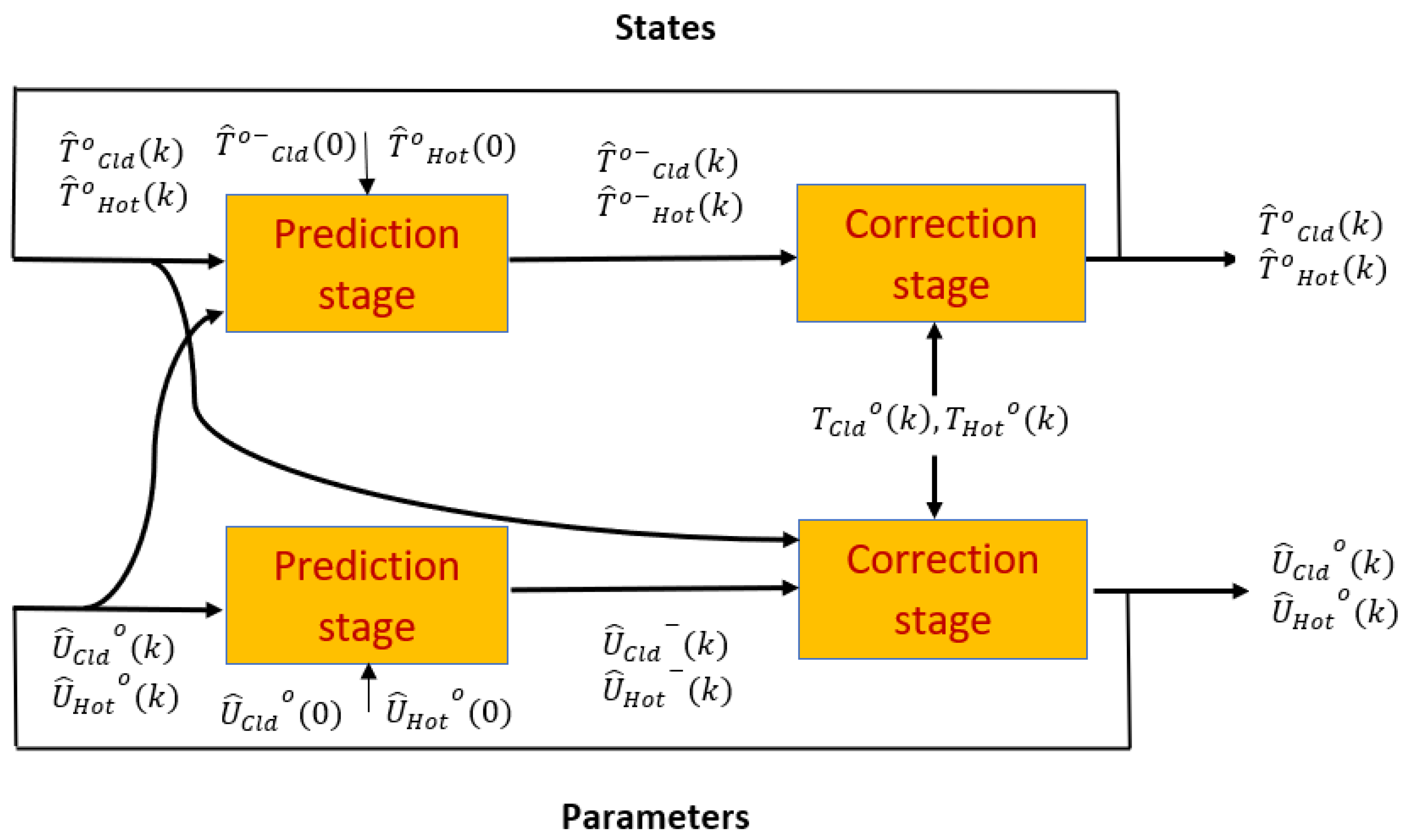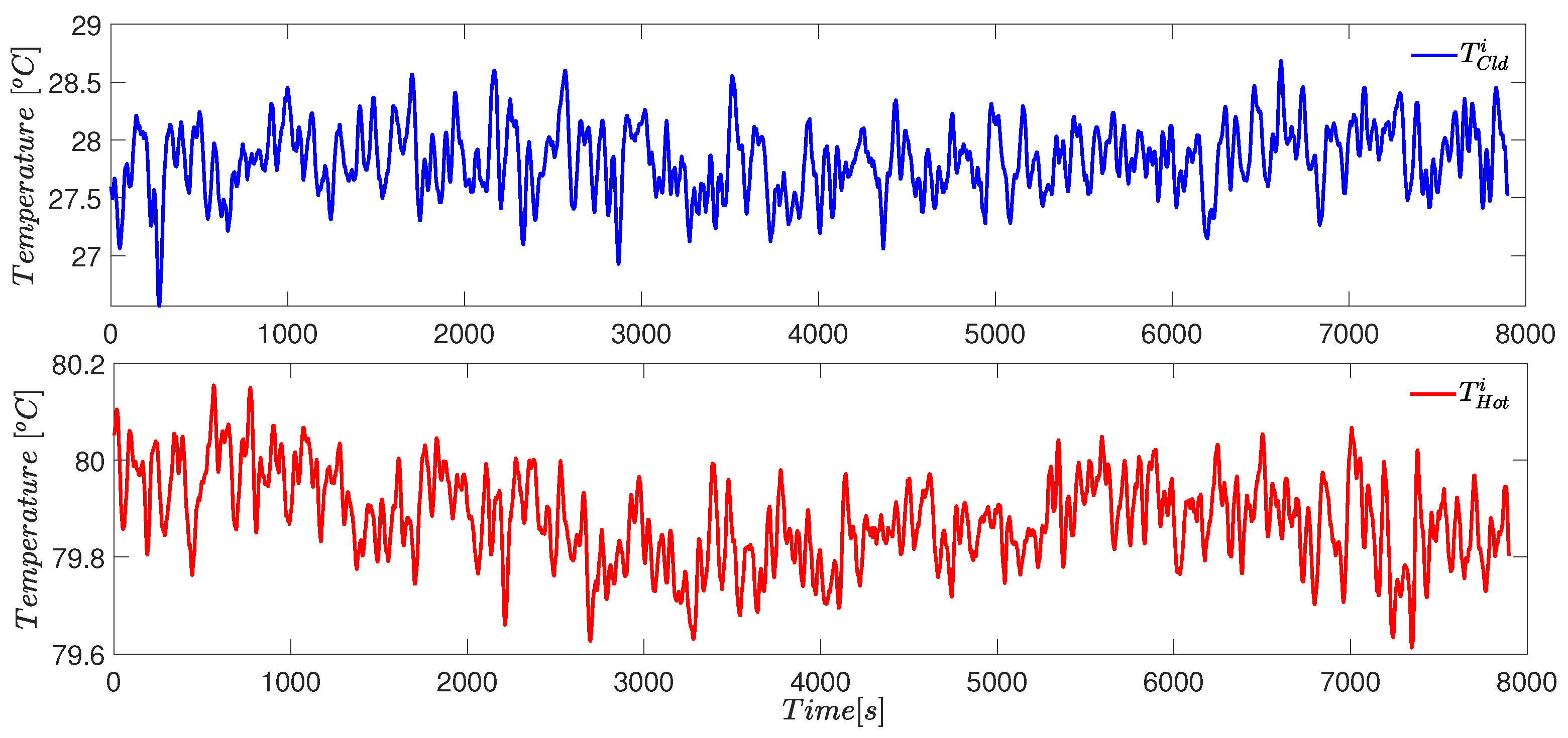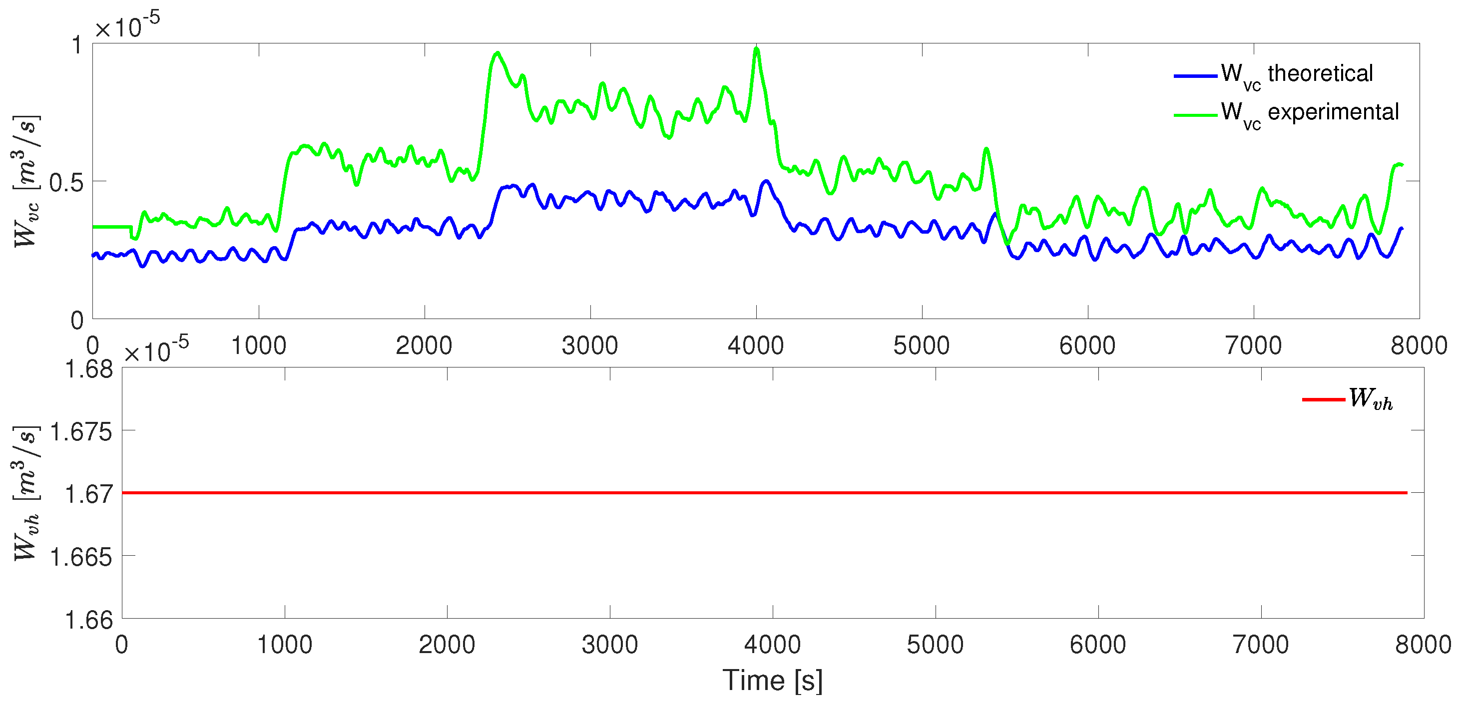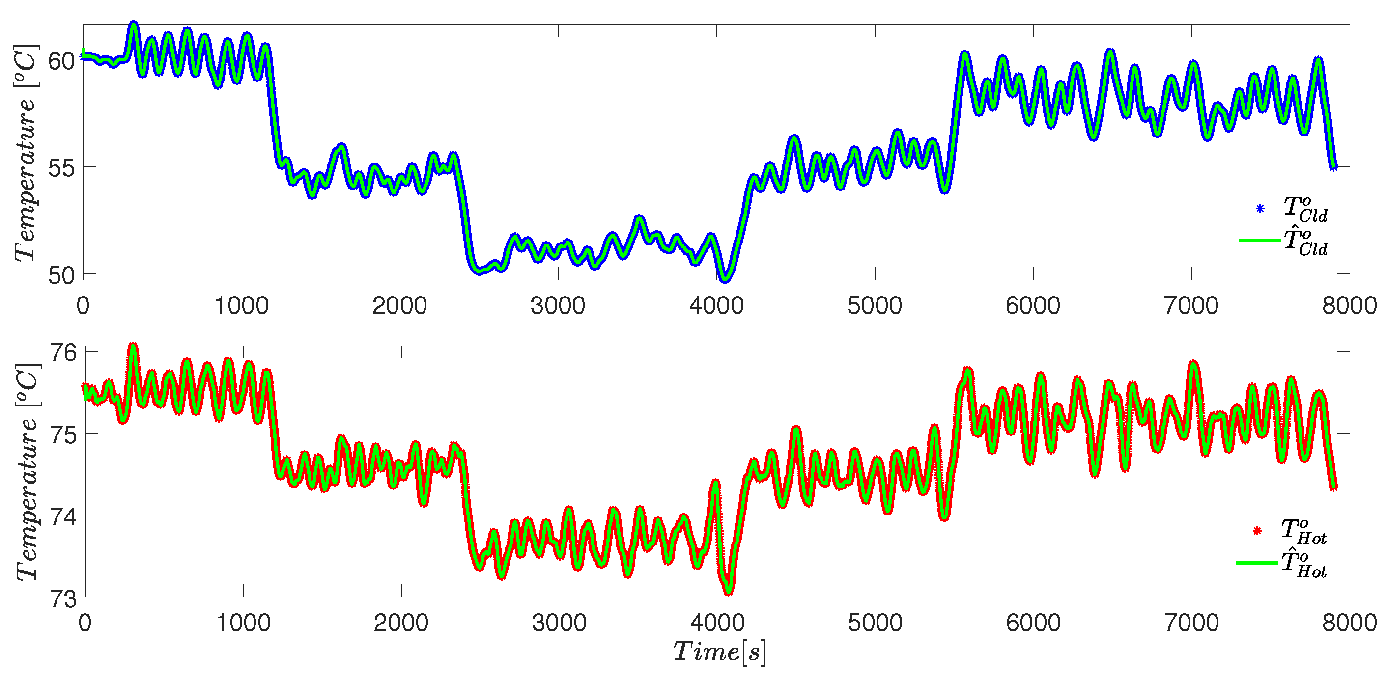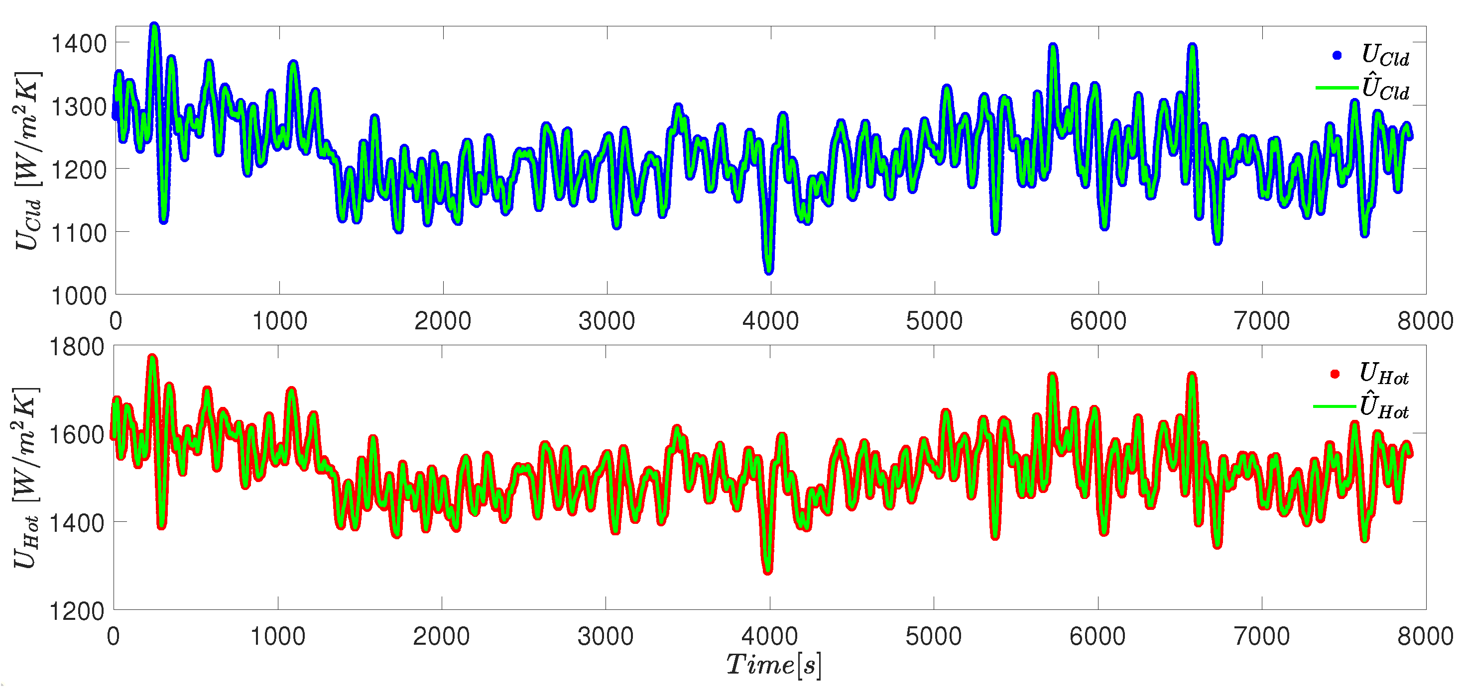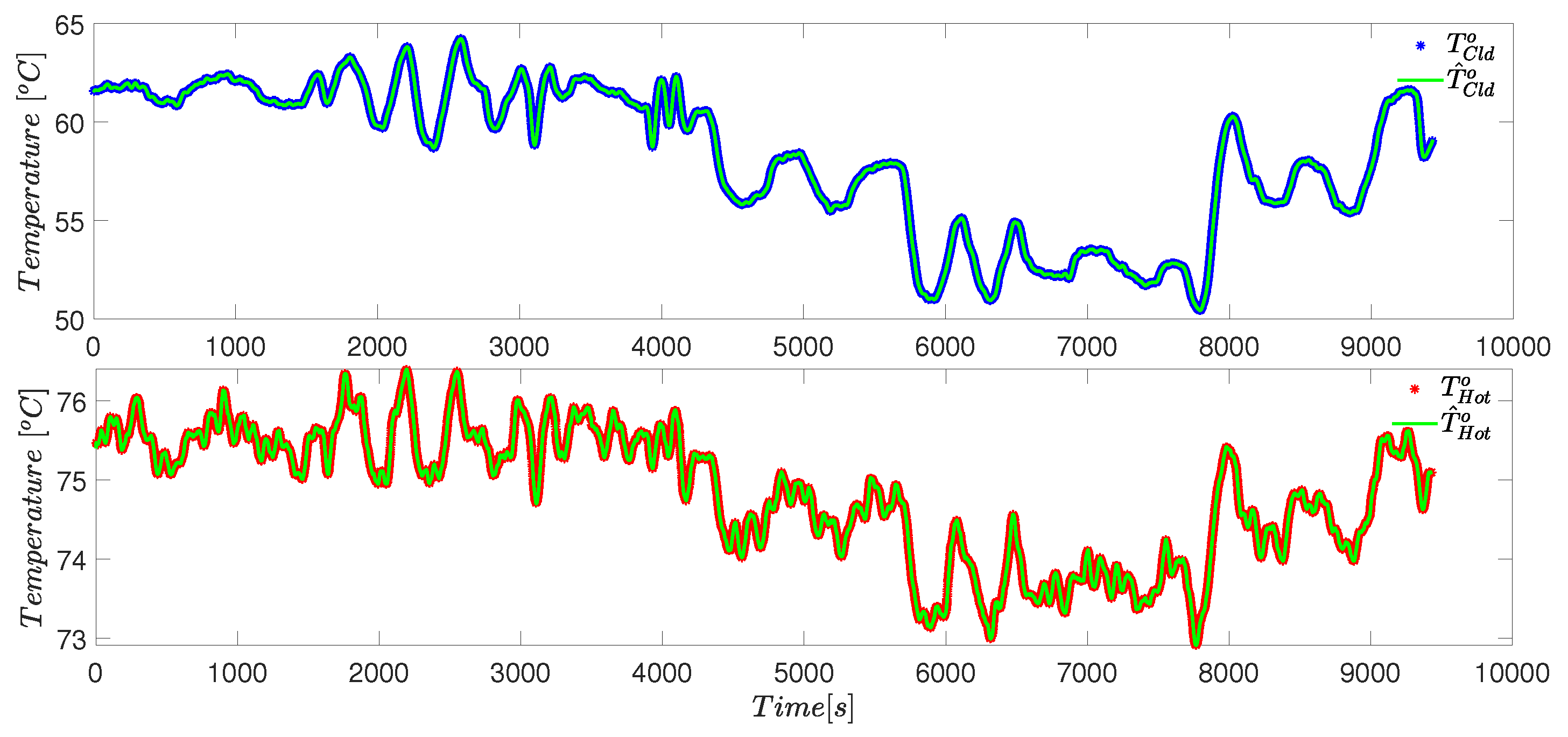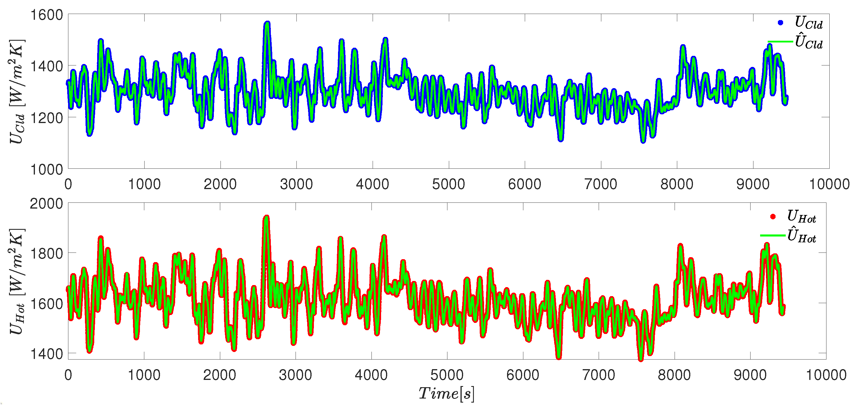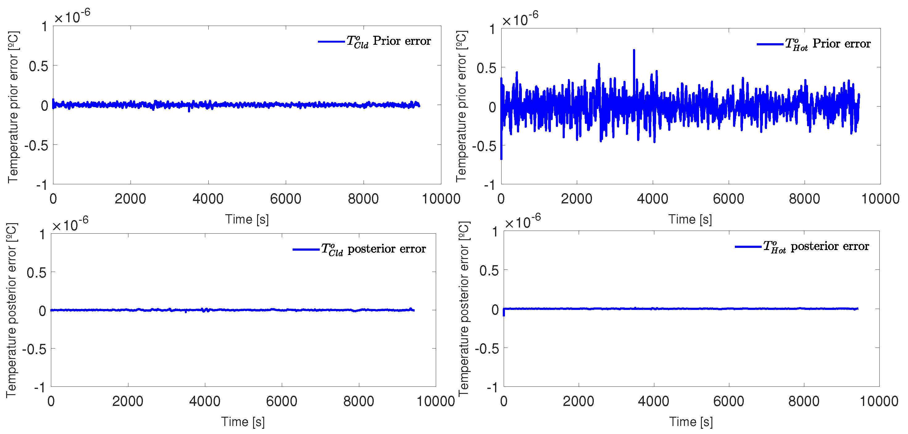25]. Therefore, DEKF appears suitable for implementation in heat exchangers. Hence, in this work, the online estimation of the temperatures and heat transfer coefficients of a heat exchanger using the DEKF was carried out. The estimations were carried out at two experimental tests, where the cold mass flow rates were varied along the tests. The estimated values of the heat transfer coefficients were compared with values calculated by algebraic equations. For concluding the results section, an error analysis of the estimated temperatures and heat transfer coefficients was presented.

2. Materials and Methods

The double-pipe heat exchanger (HE) is shown in Figure 1. The heat exchanger bench is a Didatec RCT-100 manufactured in France, which includes two control valves and four Pt-100 temperature sensors. The HE consists of two concentric circular tubes, where the hot water flows in the internal tube, while the cold fluid flows in the annular space between the tubes. The fluids circulate in counter-flow. The experimental tests were performed under two heat exchanger conditions. In the first condition, the heat exchanger was fouled, and organic materials were present on the walls and the heat exchanger flowmeter. Therefore, the heat exchanger was cleaned to perform the second test under cleaning conditions.

2.1. Mathematical Model

The energy balances that describe the dynamic of the system are shown in Equation (1) [26].

$$\begin{array}{cc}\hfill & {\displaystyle \frac{d{T}_{Cld}^o}{dt}}={\displaystyle \frac{W{v}_{Cld}}{V_{Cld}}}\left(T_{Cld}^i\left(t\right)-T_{Cld}^o\left(t\right)\right)+\left({\displaystyle \frac{U_{Cld}{A}_{Cld}}{C{p}_{Cld}{\rho }_{Cld}{V}_{Cld}}}\right)\left(T_{Hot}^o\left(t\right)-T_{Cld}^o\left(t\right)\right),\hfill \\ \hfill & {\displaystyle \frac{d{T}_{Hot}^o}{dt}}={\displaystyle \frac{W{v}_{Hot}}{V_{Hot}}}\left(T_{Hot}^i\left(t\right)-T_{Hot}^o\left(t\right)\right)+\left({\displaystyle \frac{U_{Hot}{A}_{Hot}}{C{p}_{Hot}{\rho }_{Hot}{V}_{Hot}}}\right)\left(T_{Cld}^o\left(t\right)-T_{Hot}^o\left(t\right)\right),\hfill \end{array}$$

(1)

where T, $Wv$, V, A, $Cp$, and $\rho$ are the temperature, volumetric flow, specific volume, transfer area, specific heat capacity, and density, respectively. The subscripts $Cld$ and $Hot$ correspond to the cold and hot streams, respectively, and the superscripts i and o correspond to the inlet and outlet, respectively.

The heat transfer coefficient U is obtained by an algebraic equation, which is shown in Equation (2).

$$U_{Cld,Hot}=Q_{Cld,Hot}/A(\Delta T_{st}),$$

(2)

where $\Delta T_{st}$ is the temperature difference between the streams, and ${\dot{Q}}_{Hot,Cld}$ is the heat transferred from the hot fluid or received from the cold fluid, which is calculated by Equation (3). In Equation (3), $\Delta T$ corresponds to the temperature difference between the inlet and outlet of each stream.

$${\dot{Q}}_{Hot,Cld}=W{m}_{Hot,Cld}C{p}_{Hot,Cld}(\Delta T_{Hot,Cld}).$$

(3)

2.2. Cold Mass Flow Rate Calculation

The cold mass flow rate was not measured experimentally because the fouling affects the flowmeter of the cold stream, which produces incorrect measurements. Therefore, the calculation of the cold mass flow rate was carried out using Equation (4). This equation was obtained by isolating the cold mass flow rate from Equation (5), which considers that the heat transfer rate accepted by the cold side equals the heat transfer rate released by the hot side (${\dot{Q}}_c={\dot{Q}}_h$).

$$W{m}_{Cld}={\displaystyle \frac{W{m}_{Hot}C{p}_{Hot}(\Delta T_{Hot})}{C{p}_{Cld}(\Delta T_{Cld})}},$$

(4)

$$W{m}_{Cld}C{p}_{Cld}(\Delta T_{Cld})=W{m}_{Hot}C{p}_{Hot}(\Delta T_{Hot}).$$

(5)

2.3. Dual-Extended Kalman Filter Design

The dual-extended Kalman filter (DEKF) provides an initialization procedure for combined state and parameter estimation by using two extended Kalman filters (EKFs) in parallel. Whereas the EKF estimates only the state, the DEKF estimates both the state and the unknown parameters that can affect the behavior of the system [27]. Equations (6)–(9) show the DEKF equations representing the prediction and correction steps [13].

State prediction:

$$\begin{array}{cc}\hfill & {\widehat{x}}_{state}^{-}\left(k\right)=f({\widehat{x}}_{state}^{-}\left(k-1\right),u\left(k\right),{\widehat{x}}_{par}^{-}\left(k\right)),\hfill \\ \hfill & {\Phi }_{state}^{-}\left(k\right)=J_{state}\left(k\right){\Phi }_{state}^{-}(k-1)J_{state}^T\left(k\right)+R_I.\hfill \end{array}$$

(6)

State correction:

$$\begin{array}{cc}\hfill & K_{state}\left(k\right)={\Phi }_{state}^{-}\left(k\right)H_{state}^T{\left[{\sigma }_{state}+H_{state}{\Phi }_{state}^{-}\left(k\right)H_{state}^T\right]}^{-1},\hfill \\ \hfill & {\widehat{x}}_{state}\left(k\right)={\widehat{x}}_{state}^{-}\left(k\right)+K_{state}\left(k\right)\left[y\left(k\right)-H_{state}{\widehat{x}}_{state}^{-}\left(k\right)\right],\hfill \\ \hfill & {\Phi }_{state}\left(k\right)=\left[I-K_{state}\left(k\right)H_s\right]{\Phi }_{state}^{-}\left(k\right).\hfill \end{array}$$

(7)

Parameter prediction:

$$\begin{array}{cc}\hfill & {\widehat{x}}_{par}^{-}\left(k\right)={\widehat{x}}_{par}(k-1),\hfill \\ \hfill & {\Phi }_{par}^{-}\left(k\right)={\Phi }_{par}^{-}(k-1)+R_n.\hfill \end{array}$$

(8)

Parameter correction:

$$\begin{array}{cc}\hfill & K_{par}\left(k\right)={\Phi }_{par}^{-}\left(k\right)H_{par}^T{\left[{\sigma }_p+H_{par}{\Phi }_{par}^{-}\left(t\right)H_{par}^T\right]}^{-1},\hfill \\ \hfill & {\widehat{x}}_{par}\left(k\right)={\widehat{x}}_{par}^{-}\left(k\right)+K_{par}\left(k\right)\left[y\left(k\right)-H_{state}{\widehat{x}}_{state}^{-}\left(k\right)\right],\hfill \\ \hfill & {\Phi }_{par}\left(k\right)=\left[I-K_{par}\left(k\right)H_{par}\right]{\Phi }_{par}^{-}\left(t\right),\hfill \end{array}$$

(9)

where $R_I$ and $R_n$ are covariance matrices of the process noise for the states and parameters, respectively. ${\sigma }_{state}$ and ${\sigma }_{par}$ are covariance matrices of the output noise, and ${\Phi }_{state}$ and ${\Phi }_{par}$ are covariance matrices of the estimation error. $K_{state}$ and $K_{par}$ are the Kalman gain matrices for the states and parameters, respectively. $J_{state}$ is the Jacobian matrix for the state, and $H_{par}$ is the Jacobian matrix concerning the parameter. $H_{state}$ is the Jacobian matrix of the output equations.

2.4. Stability and Convergence

To demonstrate stability and convergence, let us define a discrete-time nonlinear system as follows.

$$\begin{array}{c}x\left(k+1\right)=f(x\left(k\right),u\left(k\right)),\hfill \\ y\left(k\right)=h\left(x\left(k\right)\right),\hfill \end{array}$$

(10)

where x, u, are the state and the input vectors, respectively, and y is the output vector. h is a real analytic function on ${\mathcal{R}}^n$.

Meanwhile, a discrete nonlinear recursive observer can be defined as shown in Equation (11) [28].

$$\begin{array}{c}{x}^{-}\left(k+1\right)=f(\widehat{x}\left(k\right),u\left(k\right)),\hfill \\ \widehat{x}\left(k\right)=x^{-}\left(k\right)+K\left(k\right)\left(y\left(k\right)-Cx\left(k\right)\right),\hfill \end{array}$$

(11)

where the a priori and a posteriori estimates are defined by $x^{-}$ and $\widehat{x}$, respectively, and the observer gain matrix is described by $K\left(k\right)$.

The prior and posterior errors are defined by the following system equations.

$$\begin{array}{c}\zeta \left(k\right)=x\left(k\right)-x^{-}\left(k\right),\hfill \\ \eta \left(k\right)=x\left(k\right)-\widehat{x}\left(k\right).\hfill \end{array}$$

(12)

The prior ($\zeta$) and posterior ($\eta$) errors are related as is shown in the Equation (13),

$$\begin{array}{c}\eta \left(k\right)=(I-K\left(k\right)C)\zeta \left(k\right).\hfill \end{array}$$

(13)

Considering Equations (11) and (10), the nonlinear functions difference is calculated as follows:

$$f(x\left(k\right),u\left(k\right))-f(\widehat{x}\left(k\right),u\left(k\right))=J_{state}\left(k\right)\eta \left(k\right)+\rho (x\left(k\right),\widehat{x}\left(k\right),u\left(k\right)),$$

(14)

where $\rho$ represents the higher term, and $J_{state}\left(k\right)$ is a $n\times n$ matrix that represents the system linearization.

Considering Equations (10), (11), (13), and (14), the prior error can be represented as follows.

$$\begin{array}{c}x\left(k+1\right)-x^{-}\left(k+1\right)=\zeta \left(k+1\right),\hfill \\ \zeta \left(k+1\right)=J_{state}\left(k\right)\eta \left(k\right)+\rho (x\left(k\right),\widehat{x}\left(k\right),u\left(k\right)),\hfill \end{array}$$

(15)

$$\begin{array}{c}\zeta \left(k+1\right)=J_{state}\left(k\right)\left(I-K\left(k\right)C\right)\zeta \left(k\right)+r_s\left(k\right),\hfill \\ r_s\left(k\right)=\rho (x\left(k\right),\widehat{x}\left(k\right),u\left(k\right)).\hfill \end{array}$$

(16)

Now, by applying Equation (13), the dynamic of the posterior error is proposed in Equation (18), considering that the system is observable, as well as that the matrix resulting of Equation (17) is non-sigular.

$$\left(I-K\left(k\right)C\right),$$

(17)

$$\eta \left(k\right)=\left(I-K\left(k\right)C\right)\left(J_{state}(k-1)\eta \left(k-1\right)+r_s(k-1)\right).$$

(18)

Therefore, to demonstrate the local asymptotical stability of the observer given in (9), the prior (16) and posterior error (18) dynamics must tend to zero.

2.5. DEKF Implementation

Figure 2 shows a scheme of DEKF applied to estimate the temperature and the heat transfer coefficients. The detailed description of the implemented DEKF is presented as follows. The input vector u is defined in Equation (19) and the output vector y is defined in Equation (20).

$$u=\left[\begin{array}{c}W{v}_{Cld}\\ W{v}_{Hot}\end{array}\right],$$

(19)

$$y=\left[\begin{array}{c}{T}_{Cld}^o\\ T_{Hot}^o\end{array}\right]=H_s{x}_s,$$

(20)

where $H_s$ is shown in Equation (21).

$$H_s=\left[\begin{array}{cc}1& 0\\ 0& 1\end{array}\right].$$

(21)

The state and parameter vectors of the system are defined as follows:

$$x_s=\left[\begin{array}{c}{T}_{Cld}^o\\ T_{Hot}^o\end{array}\right],$$

(22)

$$x_p=\left[\begin{array}{c}{U}_c\\ U_h\end{array}\right].$$

(23)

For the state prediction stage, a discretization of the system using the Euler method is carried out, as presented in Equation (24).

$${\widehat{x}}_s^{-}=\left[\begin{array}{c}{\widehat{T}}_{Cld}^{o-}\\ {\widehat{T}}_{Hot}^{o-}\end{array}\right]=\left[\begin{array}{c}{\widehat{T}}_{Cld}^o\left(t_{k-1}\right)\\ {\widehat{T}}_{Hot}^o\left(t_{k-1}\right)\end{array}\right]+\delta \left[\begin{array}{c}{\displaystyle \frac{W{v}_{Cld}}{V_{Cld}}}\left(T_{Cld}^i\left(k\right)-T_{Cld}^o\left(k\right)\right)+\left({\displaystyle \frac{U_{Cld}{A}_{Cld}}{C{p}_{Cld}{\rho }_{Cld}{V}_{Cld}}}\right)\left(T_{Hot}^o\left(k\right)-T_{Cld}^o\left(k\right)\right)\\ {\displaystyle \frac{W{v}_{Hot}}{V_{Hot}}}\left(T_{Hot}^i\left(k\right)-T_{Hot}^o\left(k\right)\right)+\left({\displaystyle \frac{U_{Hot}{A}_{Hot}}{C{p}_{Hot}{\rho }_{Hot}{V}_{Hot}}}\right)\left(T_{Cld}^o\left(k\right)-T_{Hot}^o\left(k\right)\right)\end{array}\right],$$

(24)

where $\delta$ is the step size.

For the prediction of the covariance matrix, the Jacobian matrix $J_s$ for the state is calculated by Equation (25)

$$\begin{array}{ccc}\hfill J_s& =\left[\begin{array}{ccc}{\displaystyle \frac{\partial f_1}{\partial x_1}}& \cdots & {\displaystyle \frac{\partial f_1}{\partial x_m}}\\ ⋮& & ⋮\\ {\displaystyle \frac{\partial f_m}{\partial x_1}}& \cdots & {\displaystyle \frac{\partial f_m}{\partial x_m}}\end{array}\right]\hfill & =\left[\begin{array}{c}-{\displaystyle \frac{W{v}_{Cld}}{V_{Cld}}}-{\displaystyle \frac{U_{Cld}{A}_{Cld}}{{\rho }_{Cld}C{p}_{Cld}{V}_{Cld}}}{\displaystyle \frac{U_{Cld}{A}_{Cld}}{{\rho }_{Cld}C{p}_{Cld}{V}_{Cld}}}\\ \\ {\displaystyle \frac{U_{Hot}{A}_{Hot}}{{\rho }_{Hot}C{p}_{Hot}{V}_{Hot}}}-{\displaystyle \frac{W{v}_{Hot}}{V_{Hot}}}-{\displaystyle \frac{U_{Hot}{A}_{Hot}}{{\rho }_{Hot}C{p}_{Hot}{V}_{Hot}}}\end{array}\right]\hfill \end{array}.$$

(25)

Therefore, the covariance matrix described in Equation (6) is calculated by Equation (26).

$$\begin{array}{c}\hfill {\Phi }_s^{-}\left(t\right)=\left[\begin{array}{c}-{\displaystyle \frac{W{v}_{Cld}}{V_{Cld}}}-{\displaystyle \frac{U_{Cld}{A}_{Cld}}{{\rho }_{Cld}C{p}_{Cld}{V}_{Cld}}}{\displaystyle \frac{U_{Cld}{A}_{Cld}}{{\rho }_{Cld}C{p}_{Cld}{V}_{Cld}}}\\ \\ {\displaystyle \frac{U_{Hot}{A}_{Hot}}{{\rho }_{Hot}C{p}_{Hot}{V}_{Hot}}}-{\displaystyle \frac{W{v}_{Hot}}{V_{Hot}}}-{\displaystyle \frac{U_{Hot}{A}_{Hot}}{{\rho }_{Hot}C{p}_{Hot}{V}_{Hot}}}\end{array}\right]{\Phi }_s^{-}\left(t_{k-1}\right){\left[\begin{array}{c}-{\displaystyle \frac{W{v}_{Cld}}{V_{Cld}}}-{\displaystyle \frac{U_{Cld}{A}_{Cld}}{{\rho }_{Cld}C{p}_{Cld}{V}_{Cld}}}{\displaystyle \frac{U_{Cld}{A}_{Cld}}{{\rho }_{Cld}C{p}_{Cld}{V}_{Cld}}}\\ \\ {\displaystyle \frac{U_{Hot}{A}_{Hot}}{{\rho }_{Hot}C{p}_{Hot}{V}_{Hot}}}-{\displaystyle \frac{W{v}_{Hot}}{V_{Hot}}}-{\displaystyle \frac{U_{Hot}{A}_{Hot}}{{\rho }_{Hot}C{p}_{Hot}{V}_{Hot}}}\end{array}\right]}^T+R_I.\end{array}$$

(26)

For the state correction, the Equations (27)–(29) are used.

$$K_s\left(t\right)={\Phi }_s^{-}\left(k\right){\left[\begin{array}{cc}1& 0\\ 0& 1\end{array}\right]}^T{\left[{\sigma }_s+\left[\begin{array}{cc}1& 0\\ 0& 1\end{array}\right]{\Phi }_s^{-}\left(k\right){\left[\begin{array}{cc}1& 0\\ 0& 1\end{array}\right]}^T\right]}^{-1},$$

(27)

$$\left[\begin{array}{c}{\widehat{T}}_{Cld}^o\left(k\right)\\ {\widehat{T}}_{Hot}^o\left(k\right)\end{array}\right]=\left[\begin{array}{c}{\widehat{T}}_{Cld}^{o-}\left(k\right)\\ {\widehat{T}}_{Hot}^{o-}\left(k\right)\end{array}\right]+K_s\left(k\right)\left[\left[\begin{array}{c}{T}_{Cld}^o\left(k\right)\\ T_{Hot}^o\left(k\right)\end{array}\right]-\left[\begin{array}{cc}1& 0\\ 1& 0\end{array}\right]\left[\begin{array}{c}{\widehat{T}}_{Cld}^{o-}\left(k\right)\\ {\widehat{T}}_{Hot}^{o-}\left(k\right)\end{array}\right]\right],$$

(28)

$${\Phi }_s\left(k\right)=\left[\left[\begin{array}{cc}1& 0\\ 1& 0\end{array}\right]-K_s\left(k\right)\left[\begin{array}{cc}1& 0\\ 1& 0\end{array}\right]\right]{\Phi }_s^{-}\left(k\right).$$

(29)

The parameter predictions are calculated with Equations (30) and (31).

$$\left[\begin{array}{c}{\widehat{U}}_{Cld}^{-}\left(k\right)\\ {\widehat{U}}_{Hot}^{-}\left(k\right)\end{array}\right]=\left[\begin{array}{c}{\widehat{U}}_{Cld}(k-1)\\ {\widehat{U}}_{Hot}(k-1)\end{array}\right],$$

(30)

$${\Phi }_p^{-}\left(k\right)={\Phi }_p^{-}(k-1)+R_n.$$

(31)

For the parameter correction, the Jacobian matrix concerning the parameters is calculated with Equation (32).

$$\begin{array}{cc}\hfill H_p& =H_s·{\displaystyle \frac{\partial f({\widehat{x}}_s,{\widehat{x}}_p)}{\partial {\widehat{x}}_p}},\hfill \\ \hfill & =H_s\left[\begin{array}{cc}{\displaystyle \frac{A_{Cld}}{{\rho }_{Cld}C{p}_{Cld}{V}_{Cld}}}\left(T_{Hot}^o\left(k\right)-T_{Cld}^o\left(k\right)\right)& 0\\ 0& {\displaystyle \frac{A_{Hot}}{{\rho }_{Hot}C{p}_{Hot}{V}_{Hot}}}\left(T_{Cld}^o\left(k\right)-T_{Hot}^o\left(k\right)\right)\end{array}\right].\hfill \end{array}$$

(32)

The Kalman gain matrix for the parameter, the parameter correction, and the covariance matrix of the estimation error are calculated with Equations (33)–(35).

$$\begin{array}{cc}\hfill K_p\left(t\right)=& {\Phi }_p^{-}\left(k\right){\left[\begin{array}{cc}{\displaystyle \frac{A_{Cld}}{{\rho }_{Cld}C{p}_{Cld}{V}_{Cld}}}\left(T_{Hot}^o\left(k\right)-T_{Cld}^o\left(k\right)\right)& 0\\ 0& {\displaystyle \frac{A_{Hot}}{{\rho }_{Hot}C{p}_{Hot}{V}_{Hot}}}\left(T_{Cld}^o\left(k\right)-T_{Hot}^o\left(k\right)\right)\end{array}\right]}^T\hfill \\ \hfill & [{\sigma }_p+\left[\begin{array}{cc}{\displaystyle \frac{A_{Cld}}{{\rho }_{Cld}C{p}_{Cld}{V}_{Cld}}}\left(T_{Hot}^o\left(k\right)-T_{Cld}^o\left(k\right)\right)& 0\\ 0& {\displaystyle \frac{A_{Hot}}{{\rho }_{Hot}C{p}_{Hot}{V}_{Hot}}}\left(T_{Cld}^o\left(k\right)-T_{Hot}^o\left(k\right)\right)\end{array}\right]\hfill \\ \hfill & {\Phi }_p^{-}\left(k\right){\left[\begin{array}{cc}{\displaystyle \frac{A_{Cld}}{{\rho }_{Cld}C{p}_{Cld}{V}_{Cld}}}\left(T_{Hot}^o\left(k\right)-T_{Cld}^o\left(k\right)\right)& 0\\ 0& {\displaystyle \frac{A_{Hot}}{{\rho }_{Hot}C{p}_{Hot}{V}_{Hot}}}\left(T_{Cld}^o\left(k\right)-T_{Hot}^o\left(k\right)\right)\end{array}\right]}^T{]}^{-1},\hfill \end{array}$$

(33)

$$\begin{array}{c}\hfill \left[\begin{array}{c}{\widehat{U}}_{Cld}\left(k\right)\\ {\widehat{U}}_{Hot}\left(k\right)\end{array}\right]=\left[\begin{array}{c}{\widehat{U}}_{Cld}^{-}\left(k\right)\\ {\widehat{U}}_{Hot}^{-}\left(k\right)\end{array}\right]+K_p\left(k\right)\left[\left[\begin{array}{c}{\widehat{T}}_{Cld}^o\left(k\right)\\ {\widehat{T}}_{Hot}^o\left(k\right)\end{array}\right]-\left[\begin{array}{cc}1& 0\\ 0& 1\end{array}\right]\left[\begin{array}{c}{\widehat{T}}_{Cld}^{o-}\left(k\right)\\ {\widehat{T}}_{Hot}^{o-}\left(k\right)\end{array}\right]\right]\end{array},$$

(34)

$$\begin{array}{c}\hfill \begin{array}{cc}& {\Phi }_p\left(k\right)=\left[\left[\begin{array}{cc}1& 0\\ 0& 1\end{array}\right]-K_p\left(k\right)\left[\begin{array}{cc}{\displaystyle \frac{A_{Cld}}{{\rho }_{Cld}C{p}_{Cld}{V}_{Cld}}}\left(T_{Hot}^o\left(k\right)-T_{Cld}^o\left(k\right)\right)& 0\\ 0& {\displaystyle \frac{A_{Hot}}{{\rho }_{Hot}C{p}_{Hot}{V}_{Hot}}}\left(T_{Cld}^o\left(k\right)-T_{Hot}^o\left(k\right)\right)\end{array}\right]\right]\hfill \end{array}\hspace{1em}{\Phi }_p^{-}\left(k\right).\end{array}$$

(35)

3. Results

This section presents the experimental results of implementing the dual-extended Kalman filter (DEKF) to estimate the heat transfer coefficient in the heat exchanger. The tests were carried out experimentally under two operating conditions: in the first condition, the inlet temperatures were without perturbation. In the second operating condition, the cold-water inlet temperature was perturbed by the environmental heat.

3.1. Experimental Results of the Heat Transfer Coefficients Estimations of the First Test

Figure 3 shows the temperature dynamics of the inlet cooling and hot water temperature. During the first test, the heat exchanger cooling and hot water inlet temperatures were as follows: the inlet cooling water temperature $T_{Cld}^i$ varied between 26.56 °C and 28.68 °C. This variation is due to the environmental conditions. On the other hand, the inlet hot water temperature $T_{Hot}^i$ varied between 79.61 °C and 80.15 °C.

The cooling water volumetric flow rate during the experimental test is shown in Figure 4. The green line corresponds to the measured cooling water volumetric flow rate. However, the fouling affects the heat exchanger, and, therefore, incorrect measurements may have occurred due to this fact. Hence, the cooling water volumetric flow rate was calculated using Equation (4), which considers that the heat transfer of the cold side must be equal to that of the hot side. The blue line shows the cooling water volumetric flow rate calculated by Equation (4). At the beginning of the test, the cooling water volumetric flow rate ($W_{vc}$) was $2.36\times {10}^{-6}$ m³/s. From time 1 s to 1179 s, the average cooling water volumetric flow rate was $2.2897\times {10}^{-6}$ m³/s. Subsequently, the $W_{vc}$ was increased, reaching $3.255\times {10}^{-6}$ m³/sat time 1240 s. The average $W_{vc}$ was $3.2968\times {10}^{-6}$ m³/s from time 1240 s to 2380 s. Then, at time 2333 s, a new volumetric flow rate change is performed, and the value of $W_{vc}$ increased; the maximum value was reached at time 2533 s, and the $W_{vc}$ was $4.842\times {10}^{-6}$ m³/s. In this operating condition, the average $W_{vc}$ was $4.3496\times {10}^{-6}$ m³/s. Two more operating points were selected, at times 4144 s and 5485 s. The average cooling water volumetric flow rates were $3.2678\times {10}^{-6}$ m³/s and $2.5728\times {10}^{-6}$ m³/s. Meanwhile, the hot water volumetric flow rate was constant at $1.67\times {10}^{-5}$ m³/s, as shown at the bottom of Figure 4.

The behavior of the cooling and hot water outlet temperatures $T_{Cld}^o$ and $T_{Hot}^o$ at different operating conditions is shown in Figure 5. At the top and bottom of the figure, in the blue and red lines, the measured cooling water outlet temperature $T_{Cld}^o$ and the measured hot water outlet temperature $T_{Hot}^o$ are shown, respectively. The green lines correspond to the estimated temperatures ${\widehat{T}}_{Cld}^o$ and ${\widehat{T}}_{Hot}^o$.

Table 1. Measured and estimated temperatures in the first test.

Variable	OP 1	OP 2	OP 3	OP 4	OP 5
$T_{Cld}^o$	60.1062	54.6148	51.0887	55.0344	58.1967
$T_{Hot}^o$	75.5192	74.5805	73.6707	74.4928	75.1904
${\widehat{T}}_{Cld}^o$	60.1073	54.6158	51.0882	55.0328	58.1978
${\widehat{T}}_{Hot}^o$	75.5193	74.5803	73.6706	74.4927	75.1907

shows an average of measured temperatures $T_{Cld}^o$ and $T_{Hot}^o$ and estimated ${\widehat{T}}_{Cld}^o$ and ${\widehat{T}}_{Hot}^o$ for each operating condition (OP). The mean errors between the measured and estimated temperatures are shown in

Table 2. Mean errors between the measured and estimated temperatures for each operating condition in the first test.

Variable	OP 1	OP 2	OP 3	OP 4	OP 5
${\left(\overline{T-\widehat{T}}\right)}_{Cld}^o$	$-1.20\times {10}^{-3}$	$-1.00\times {10}^{-3}$	$5.10\times {10}^{-4}$	$1.60\times {10}^{-3}$	$-1.10\times {10}^{-3}$
${\left(\overline{T-\widehat{T}}\right)}_{Hot}^o$	$-9.01\times {10}^{-5}$	$2.15\times {10}^{-4}$	$8.12\times {10}^{-5}$	$1.21\times {10}^{-4}$	$-3.16\times {10}^{-4}$

.

Finally, the experimental results of the heat transfer coefficients (HTC) estimation with the DEKF and the one calculated by the algebraic equation are shown in Figure 6. In the figure, the green lines correspond to the HTC estimated by the DEKF, and the blue and red lines correspond to the heat transfer coefficient calculated by the algebraic equations. The figure shows the same behavior between the HTC estimation carried out by the DEFK and the algebraic method. The minimum and maximum values of the heat transfer coefficients were between $1.0370\times {10}^3$ W/m² °C and $1.4256\times {10}^3$ W/m² °C for the cold side and $1.2879\times {10}^3$ W/m² °C and $1.7706\times {10}^3$ W/m² °C for the hot side, as shown in Figure 6.

Table 3. Algebraic and estimated heat transfer coefficients in the first test.

Variable	OP 1	OP 2	OP 3	OP 4	OP 5
$U_{Cld}$	$1.2807\times {10}^3$	$1.1811\times {10}^3$	$1.2036\times {10}^3$	$1.2229\times {10}^3$	$1.2223\times {10}^3$
$U_{Hot}$	$1.5906\times {10}^3$	$1.4668\times {10}^3$	$1.4948\times {10}^3$	$1.5188\times {10}^3$	$1.5181\times {10}^3$
${\widehat{U}}_{Cld}$	$1.2808\times {10}^3$	$1.1812\times {10}^3$	$1.2036\times {10}^3$	$1.2229\times {10}^3$	$1.2224\times {10}^3$
${\widehat{U}}_{Hot}$	$1.4670\times {10}^3$	$1.4948\times {10}^3$	$1.5187\times {10}^3$	$1.5187\times {10}^3$	$1.5180\times {10}^3$

shows the average values of the algebraic ($U_{Cld}$ and $U_{Hot}$) and estimated heat transfer coefficients (${\widehat{U}}_{Cld}$ and ${\widehat{U}}_{Hot}$), and their mean errors in each operating point are shown in

Table 4. Meanerrors between the algebraic and estimated heat transfer coefficients and dispersion measures for each operating condition in the first test.

Variable	OP 1	OP 2	OP 3	OP 4	OP 5
${\left(\overline{U-\widehat{U}}\right)}_{Cld}$	−0.0604	−0.1138	0.0086	0.0793	−0.0027
$Varianc{e}_{Cld}$	13.6169	4.9228	3.2085	4.5485	9.8956
$ST{D}_{Cld}$	3.6901	2.2187	1.7912	2.1327	3.1457
$C{I}_{Cld}$	±2.8709	±2.1592	±2.3641	±2.6656	±2.2094
${\left(\overline{U-\widehat{U}}\right)}_{Hot}$	−0.1113	−0.1887	0.0048	0.1054	0.0340
$Varianc{e}_{Hot}$	33.0538	15.3765	12.2871	13.0961	24.4653
$ST{D}_{Hot}$	5.7492	3.9213	3.5053	3.6188	4.9462
$C{I}_{Hot}$	±3.5743	±2.6820	±2.9397	±3.3169	±2.7415

. Additionally, dispersion measures such as standard deviation (STD), variance, and confidence intervals (CI) were calculated to determine the uncertainty of the DEKF relative to the experimental data as shown in Table 4. The selection of $R_n$ = [5.9 $\times {10}^3$, 0; 0, 2.1] for parameter estimation ensured a precise HTC estimation as shown in Table 4 with absolute errors < 0.1887. As shown in Figure 6 at t = 1240 s, the estimated parameters fit the HTC calculated by the algebraic equation. As shown in the figure, despite the changes in the operating condition, the estimated HTC converges quickly to the value calculated by the algebraic equation. Since the DEKF was designed to describe the same behavior as given by the algebraic equations, these estimations are sensitive to the sensor’s noise. However, other selections of $R_n$ = [1.9, 0; 0, 1 $\times {10}^{-4}$] can reduce the sensor noise sensitivity.

Mean square errors between the algebraic and estimated heat transfer coefficients are given in

Table 5. Mean square errors between the algebraic and estimated heat transfer coefficients and the standard deviation of the errors in the first test.

Parameter ${\mathit{U}}_{\mathit{c}}$	Value	Parameter ${\mathit{U}}_{\mathit{h}}$	Value
MSE	0.258	MSE	3.19
STD	0.5058	STD	1.7887

. This table shows low errors, which indicates that the estimation is adequate to estimate the HTC.

3.2. Experimental Results of the Heat Transfer Coefficient Estimations of the Second Test

The heat exchanger inlet temperatures were as follows: the inlet cooling water temperature ($T_{Cld}^i$) gradually increased from 25.50 °C to 28.79 °C, as shown at the top of Figure 7. This inlet cooling water temperature varied due to ambient conditions. Meanwhile, the inlet hot water temperature ($T_{Hot}^i$) varied between 79.38 °C and 79.98 °C, as shown in the bottom of Figure 7.

The volumetric flow rates in the heat exchanger were managed as follows: the hot water flow rate was constant $1.66$ × 10⁻⁵ m³/s, and the cooling water flow rate was varied at different operating conditions between a range $1.4809\times {10}^{-6}$ m³/s to $4.9790\times {10}^{-6}$ m³/s, as shown in Figure 8. The green line corresponds to the measured cooling water volumetric flow rate using the flowmeter, while the blue line represents the cooling water volumetric flow rate calculated using Equation (4). In this case, both lines are similar because this experimental test does not present fouling.

On the other hand, Figure 9 shows the cooling and hot water outlet temperatures ($T_{Cld}^o$ and $T_{Hot}^o$). Both temperature dynamics depend on the cooling water volumetric flow rate $W_{vc}$ dynamics. The measured cooling and hot water outlet temperatures are represented by the blue and red lines, respectively. Meanwhile, the green lines correspond to the estimated temperatures. The test was performed by changing the operating conditions, first by increasing the volumetric flow rate of the cooling water temperature, and then, at time 7778 s, decreasing $W_{vc}$.

The average values of the cooling and hot water measured temperatures $T_{Cld}^o$ and $T_{Hot}^o$ and the estimated temperatures ${\widehat{T}}_{Cld}^o$ and ${\widehat{T}}_{Hot}^o$ for each operating point is shown in

Table 6. Measured and estimated temperatures in the second test.

Variable	OP 1	OP 2	OP 3	OP 4	OP 5
$T_{Cld}^o$	61.5107	56.9609	52.6660	57.1479	60.5287
$T_{Hot}^o$	75.5514	74.5573	73.6846	74.5521	75.2750
${\widehat{T}}_{Cld}^o$	61.5107	56.9610	52.6669	57.1471	60.5299
${\widehat{T}}_{Hot}^o$	75.5513	74.5571	73.6846	74.5522	75.2753

.

Table 7. Mean errors between the measured and estimated temperatures for each operating condition in the second test.

Variable	OP 1	OP 2	OP 3	OP 4	OP 5
${\left(\overline{T-\widehat{T}}\right)}_{Cld}^o$	$-3.26\times {10}^{-4}$	$-1.90\times {10}^{-3}$	$-8.77\times {10}^{-4}$	$-1.60\times {10}^{-3}$	$-8.97\times {10}^{-4}$
${\left(\overline{T-\widehat{T}}\right)}_{Hot}^o$	$-4.63\times {10}^{-5}$	$-1.55\times {10}^{-4}$	$-4.40\times {10}^{-5}$	$-8.61\times {10}^{-5}$	$-1.68\times {10}^{-4}$

shows the mean errors between the measured and estimated cooling and hot water temperatures. As shown in both tables, the DEKF accurately estimates both outlet temperatures $T_{Cld}^o$ and $T_{Hot}^o$.

Finally, the experimental results of the heat transfer coefficients with the DEKF and the one calculated by the algebraic equation are shown in Figure 10. In Figure 10, the green lines correspond to the heat transfer coefficient estimation by the DEKF, and the blue and red lines correspond to the heat transfer coefficient calculated by the algebraic equations. The minimum and maximum values of the heat transfer coefficients were between $1.1065\times {10}^3$ W/m² °C and $1.5632\times {10}^3$ W/m² °C for the cold side and $1.3743\times {10}^3$ W/m² °C and $1.9414\times {10}^3$ W/m² °C for the hot side, as shown in Figure 10.

Table 8. Algebraic and estimated heat transfer coefficients in the second test.

Variable	OP 1	OP 2	OP 3	OP 4	OP 5
$U_{Cld}$	$1.3162\times {10}^3$	$1.2874\times {10}^3$	$1.2476\times {10}^3$	$1.3198\times {10}^3$	$1.3621\times {10}^0$
$U_{Hot}$	$1.6347\times {10}^3$	$1.5988\times {10}^3$	$1.5494\times {10}^3$	$1.6391\times {10}^3$	$1.6916\times {10}^3$
${\widehat{U}}_{Cld}$	$1.3162\times {10}^3$	$1.2874\times {10}^3$	$1.2477\times {10}^3$	$1.3197\times {10}^3$	$1.3622\times {10}^3$
${\widehat{U}}_{Hot}$	$1.6347\times {10}^3$	$1.5989\times {10}^3$	$1.5495\times {10}^3$	$1.6389\times {10}^3$	$1.6916\times {10}^3$

shows the average values of the algebraic ($U_{Cld}$ and $U_{Hot}$) and estimated heat transfer coefficients (${\widehat{U}}_{Cld}$ and ${\widehat{U}}_{Hot}$), and their mean errors in each operating point are shown in

Table 9. Mean errors between the algebraic and estimated heat transfer coefficients and dispersion measures for each operating condition in the second test.

Variable	OP 1	OP 2	OP 3	OP 4	OP 5
${\left(\overline{U-\widehat{U}}\right)}_{Cld}$	−0.0055	−0.0280	0.0220	−0.0238	−0.0252
$Varianc{e}_{Cld}$	0.3811	0.3599	0.7167	0.2296	0.5664
$ST{D}_{Cld}$	0.6173	0.5999	0.8466	0.2296	0.7526
$C{I}_{Cld}$	±2.2851	±2.6382	±2.2733	±2.8008	±7.4281
${\left(\overline{U-\widehat{U}}\right)}_{Hot}$	−0.0121	−0.0014	0.0328	−0.0125	−0.0058
$Varianc{e}_{Hot}$	3.6977	2.3746	1.7088	2.5516	3.0116
$ST{D}_{Hot}$	1.9229	1.5410	1.3072	2.5516	1.7354
$C{I}_{Hot}$	±2.8373	±3.2707	±2.8124	±3.4660	±9.1983

. Additionally, dispersion measures such as standard deviation (STD), variance, and confidence intervals (CI) were calculated to determine the uncertainty of the DEKF relative to the experimental data as shown in Table 9.

Mean square errors between the measured and estimated temperatures are shown in

Table 10. Mean square errors between calculated and estimated heat transfer coefficients and the standard deviation of the errors for the second test.

Parameter ${\mathit{U}}_{\mathit{c}}$	Value	Parameter ${\mathit{U}}_{\mathit{h}}$	Value
MSE	0.4571	MSE	2.8620
STD	0.6761	STD	1.6918

, and for these calculations all data were considered. This table shows low errors, which indicates that the estimation is adequate to estimate the HTC.

To conclude the results section, Equations (16) and (18) were considered to compute the prior and the posterior errors of the cold and hot water temperatures to show the stability and convergence of the observer, as shown in Figure 11.

4. Conclusions

A dual-extended Kalman filter (DEKF) was implemented in a double pipe counter-current heat exchanger to estimate the heat transfer coefficients (HTCs). The estimator was based on the heat transfer model of the heat exchanger. Process dynamics were influenced by the variation in the cold mass flow rate, which impacted the behavior of the HTC. The estimation method showed an adequate performance since the estimated HTC presented low errors compared with the HTC calculated by algebraic equations. The results showed that the DEKF is an effective mathematical tool for detecting fouling in a heat exchanger by estimating the heat transfer coefficient.

References

1. Der, O.; Alqahtani, A.A.; Marengo, M.; Bertola, V. Characterization of polypropylene pulsating heat stripes: Effects of orientation, heat transfer fluid, and loop geometry. Appl. Therm. Eng. 2021, 184, 116304. [Google Scholar] [CrossRef]
2. Zhang, D.; He, Z.; Guan, J.; Tang, S.; Shen, C. Heat transfer and flow visualization of pulsating heat pipe with silica nanofluid: An experimental study. Heat Mass Transf. 2022, 183, 122100. [Google Scholar] [CrossRef]
3. Chen, H.; Fan, J. Decomposition based recursive least squares parameter estimation for input nonlinear equation-error systems. In Proceedings of the IEEE 36th Chinese Control Conference (CCC), Dalian, China, 26–28 July 2017; pp. 142–149. [Google Scholar]
4. Li, R.; Wang, Z.; Yu, J.; Lei, Y.; Zhang, Y.; He, J. Dynamic parameter identification of mathematical model of lithium-ion battery based on least square method. In Proceedings of the IEEE International Power Electronics and Application Conference and Exposition (PEAC), Shenzhen, China, 4–7 November 2018; pp. 1–5. [Google Scholar]
5. Li, L.; Ren, X.; Zhang, L.; Lv, Y. Adaptive parameter estimation for MISO system using decomposition principle. In Proceedings of the IEEE 8th Data Driven Control and Learning Systems Conference (DDCLS), Dali, China, 24–27 May 2019; pp. 310–315. [Google Scholar]
6. Li, M.; Zhang, L.; Liu, G. Step-wise algorithm for estimating multi-parameter of the ground and geothermal heat exchangers from thermal response tests. Renew. Energy 2020, 150, 435–442. [Google Scholar] [CrossRef]
7. Vocale, P.; Bozzoli, F.; Mocerino, A.; Navickaitė, K.; Rainieri, S. Application of an improved parameter estimation approach to characterize enhanced heat exchangers. Int. J. Heat Mass Transf. 2020, 147, 118886. [Google Scholar] [CrossRef]
8. Kivanc, O.C.; Ozturk, S.B. Sensorless PMSM drive based on stator feedforward voltage estimation improved with MRAS multiparameter estimation. IEEE/ASME Trans. Mechatron 2018, 23, 1326–1337. [Google Scholar] [CrossRef]
9. Luo, X.; Jiang, M.; Yu, L.; Fan, Y.; Zhang, L. Estimation of total heat exchange factor based on adaptive kernel density estimation theory. In Proceedings of the IEEE Chinese Control And Decision Conference (CCDC), Hefei, China, 22–24 August 2020; pp. 1015–1020. [Google Scholar]
10. Rezoug, M.R.; Taibi, D.; Benaouadj, M. State-of-charge Estimation of Lithium-ion Batteries Using Extended Kalman Filter. In Proceedings of the IEEE 10th International Conference on Power Science and Engineering (ICPSE), Istanbul, Turkey, 21–23 October 2021; pp. 98–103. [Google Scholar]
11. Idrissi, I.; Chafouk, H.; El Bachtiri, R.; Khanfara, M. Bank of Extended Kalman Filters for Faults Diagnosis in Wind Turbine Doubly Fed Induction Generator. Telkomnika 2018, 16, 2954–2966. [Google Scholar] [CrossRef]
12. Sivathanu, A.K.; Subramanian, S. Extended Kalman filter for fouling detection in thermal power plant reheater. Control Eng. Pract. 2018, 73, 91–99. [Google Scholar] [CrossRef]
13. Wenzel, T.A.; Burnham, K.; Blundell, M.V.; Williams, R.A. Dual extended Kalman filter for vehicle state and parameter estimation. Veh. Syst. Dyn. 2006, 44, 153–171. [Google Scholar] [CrossRef]
14. Zhang, J.; Chen, Y.; Xiong, J.; Zhang, L.; Hou, G. Sensor fault detection and estimation for heat exchanger using unscented Kalman filter. In Proceedings of the 9th IEEE Conference on Industrial Electronics and Applications, Hangzhou, China, 9–11 June 2014; pp. 540–545. [Google Scholar]
15. Shi, Z.; O’Brien, W. Sequential state prediction and parameter estimation with constrained dual extended Kalman filter for building zone thermal responses. Energy Build. 2008, 10, 142–149. [Google Scholar] [CrossRef]
16. Ebadollahi, S.; Khosroshahi, M. Estimating Parameters of a Dual-rate Observable Canonical System by Combining Kalman Filter and Least Squares Error Method Considering Output through Interpolation and Auxiliary Model. In Proceedings of the IEEE Iranian Conference on Electrical Engineering (ICEE), Mashhad, Iran, 8–10 May 2018; pp. 893–898. [Google Scholar]
17. Dey, A.; Dey, J. State of charge estimation of lithium-ion battery using state augmented Cubature kalman filter in presence of uncharacterized coloured noise. In Proceedings of the IEEE-HYDCON, Hyderabad, India, 11–12 September 2020; pp. 1–6. [Google Scholar]
18. Muenthong, S.; Chattakarn, S.; Lersbamrungsuk, V. Fouling Detection in Heat Exchangers using Extended Kalman Filter. IOP Conf. Ser. Mater. Sci. Eng. 2020, 778, 012083. [Google Scholar] [CrossRef]
19. Jonsson, G.; Palsson, O.P.; Sejling, K. Modeling and parameter estimation of heat exchangers—A statistical approach. J. Dyn. Sys., Meas. Control 1992, 114, 673–679. [Google Scholar] [CrossRef]
20. Jonsson, G.; Palsson, O.P. An application of extended Kalman filtering to heat exchanger models. J. Dyn. Sys. Meas. Control 1994, 116, 257–264. [Google Scholar] [CrossRef]
21. Jonsson, G.R.; Lalot, S.; Palsson, O.P.; Desmet, B. Use of extended Kalman filtering in detecting fouling in heat exchangers. Int. J. Heat Mass Transf. 2007, 50, 2643–2655. [Google Scholar] [CrossRef]
22. Canela-Sánchez, I.J.; Escobar-Jiménez, R.F.; Juárez-Romero, D. Implementation of a dual extended Kalman filter to a falling film evaporator model to optimize the process. Chem. Eng. Sci. 2024, 298, 120303. [Google Scholar] [CrossRef]
23. Paruthipulli Kalarikkal, R.M.; Subbaiah, J. Modified Dual EKF with Machine Learning Model for Fouling Prediction of Industrial Heat Exchanger. Korean J. Chem. Eng. 2024, 41, 1013–1027. [Google Scholar] [CrossRef]
24. Horváth, T.; Fodor, D. Performance Comparison of the General the Dual and the Joint Extended Kalman Filter on State Estimation of Li-ion Battery Cells for BMS. In Proceedings of the IEEE 21st International Power Electronics and Motion Control Conference (PEMC), Pilsen, Czech Republic, 30 September–3 October 2024; pp. 1–6. [Google Scholar]
25. Khodadadi, H.; Jazayeri-Rad, H. Applying a dual extended Kalman filter for the nonlinear state and parameter estimations of a continuous stirred tank reactor. Comput. Chem. Eng. 2011, 35, 2426–2436. [Google Scholar] [CrossRef]
26. Escobar, R.; Zaragoza, C.A.; Romero, D.J.; Hernández, D.; Medina, M.A. Estimación en Línea del Coeficiente de Transferencia de Calor en un Intercambiador de Calor; Asociación Mexicana de Control Automático: Zacatecas, Mexico, 2009. [Google Scholar]
27. Wan, E.A.; Nelson, A.T. Dual Extended Kalman Filter Methods. Kalman Filtering and Neural Networks; John Wiley and Sons, Inc.: Hoboken, NJ, USA, 2001. [Google Scholar]
28. Huang, R.; Patwardhan, S.C.; Biegler, L.T. Stability of a class of discrete-time nonlinear recursive observers. J. Process Control 2010, 20, 1150–1160. [Google Scholar] [CrossRef]
Figure 1. Experimental heat exchanger.
Processes 13 02117 g001
Figure 2. Scheme of the DEKF applied in the heat exchanger.
Processes 13 02117 g002
Figure 3. Inlet temperatures of the heat exchanger of the first test.
Processes 13 02117 g003
Figure 4. Cold and hot mass flow rate of the heat exchanger of the first test.
Processes 13 02117 g004
Figure 5. Cooling and hot water outlet temperatures of the heat exchanger of the first test.
Processes 13 02117 g005
Figure 6. Heat transfer coefficients of the heat exchanger of the first test.
Processes 13 02117 g006
Figure 7. Inlet temperatures of the heat exchanger of the second test.
Processes 13 02117 g007
Figure 8. Cold and hot mass flow rate of the heat exchanger of the second test.
Processes 13 02117 g008
Figure 9. Outlet temperatures of the heat exchanger of the second test.
Processes 13 02117 g009
Figure 10. Heat transfer coefficients of the heat exchanger of the second test.
Processes 13 02117 g010
Figure 11. Prior and posterior errors of the cold and hot water temperatures.
Processes 13 02117 g011