Thurstonian Model for the Difference-from-Control Test

Abstract

The difference-from-control (DFC) test is one of the sensory discrimination methods which is applicable to sensory evaluation in some areas, including process optimization and quality assessment for foods. Thurstonian models are needed for any one of the sensory discrimination methods, including the DFC. This is important because the models provide a useful sensory measure, the Thurstonian discriminal distance, $\delta$ or $d^{\prime }$, which is theoretically independent of the methods or scales used for its estimation. This paper originally derives the Thurstonian model and the estimations of the model parameters for the DFC test based on the folded normal distribution. The statistical testing, difference testing power, and sample sizes needed for the DFC test are also discussed. R codes for the estimations and tests of parameters of the model for the DFC are developed, used, and provided in the paper.

1. Introduction

The difference-from-control (DFC) test is a sensory discrimination method. It can be used to determine the degree of difference (if any) between one or more test samples and a control sample. The method is applicable to sensory evaluation in some areas, including process optimization and quality assessment for foods. The ISO standard (ISO [1]) describes the application of sensory analysis in quality control (QC) using the DFC test. For more about the DFC method, see, e.g., Muñoz et al. [2]; Costell [3]; Meilgaard et al. [4]; Kemp et al. [5]; Lawless and Heymann [6]; and Whelan [7].

In the DFC test, assessors are provided with an identified control sample, followed by one or more test samples. Blind controls are also included within this test. The assessors evaluate the identified control sample and the test sample(s) including blind controls, and scale how different they perceive the test sample(s) including blind controls to be from the identified control sample. There are different types of scales used for difference-from-control ratings. The rating can be done on a line or category scale. The scale may be a 10-point numerical scale, or a 6-point verbal scale, or a line scale with anchors, e.g., 0 and 100. The scales will range from 0 = “no difference” to 9 (or 5, or 100) = “extreme difference”. An important characteristic of the DFC test data is that all the data are positive numbers or zero, which represent the sensory intensity or distance between the test sample(s), including the blind controls, and the identified control sample, regardless of the direction of the difference.

Although the DFC test has been used in various laboratory studies, to the best knowledge of the authors, there are few, if any, discussions about a Thurstonian model for the DFC test in the sensory literature. Thurstonian models are needed for any one of the sensory discrimination methods, including the DFC. This is important because the models provide a useful sensory measure, i.e., a Thurstonian discriminal distance $\delta$ or $d^{\prime }$, which is theoretically independent of the methods or scales used for its estimation (ASTM [8]).

Bradley [9] discussed Thurstonian models for some discrimination methods including the triangle, the duo–trio, and the DFC in a memorandum prepared for the General Foods Corporation. The results were published in the statistical literature (Bradley [10]). Two indices, including the Thurstonian $\delta$ and the scaled DFC measure ${\delta }_f$, were proposed for the DFC method. However, Bradley [10] did not indicate clearly that the Thurstonian model is based on the folded normal distribution and how to estimate and test the indices of the model from the DFC test data. Bradley [10] mentioned that the methods of analysis for the DFC test data have not been entirely satisfactory. Although there have been more discussions and applications for the DFC method, the Thurstonian model for the DFC has not been discussed adequately and used widely in the sensory literature during the past 60 plus years, since this paper was published.

It should be indicated that the DFC test is also a method to determine the degree of difference of two samples. Hence, the DFC test can be regarded as another variant of the degree of difference (DOD) method. The conventional DOD includes three variants: the ratings of the A-Not A, the ratings of the A-Not A with reminder (A-Not AR), and the ratings of the Same-Different methods, which are commonly used and called in, e.g., Aust et al. [11]; Bi [12]; Bi et al. [13]; Ennis and Rousseau [14]; Ennis and Christenson [15]; Ennis [16] (Section 8.4.1); and Christensen, et al. [17]. There are three types of Thurstonian models for the three variants of the conventional DOD method. They are the Thurstonian models for the ratings of the A-Not A, the ratings of the A-Not AR, and the ratings of the Same-Different methods, which were discussed in Bi et al. [13] and Bi [18] (Sections 3.3–3.5). The Thurstonian model for the DOD in Ennis and Rousseau [14], Ennis and Christenson [15], and Christensen, et al. [17] is in fact only for a variant of the DOD, i.e., the ratings of the Same-Different method.

The main objective of this paper is to derive a Thurstonian model for the DFC method based on the folded normal distribution. Estimations including the maximum likelihood estimate and nonparametric estimate, statistical tests including difference testing and similarity/equivalence testing for the parameters of the model, and difference testing the power and sample size needed for the DFC test are also discussed and conducted. Corresponding R codes are developed, used in the paper, and provided in the Supplementary Materials.

2. Materials and Methods

2.1. Folded Normal Distribution for Perception of Difference Between Two Samples in the DFC Test

Letting $X0$ represent the perception for a test sample, $X0$ follows a normal distribution with mean ${\mu }_{x0 }$ and variance ${\sigma }^2$, i.e., $X0~N\left({\mu }_{x0 }, {\sigma }^2\right)$. Letting $Y0$ represent the perception for a control sample, $Y0$ follows a normal distribution with mean ${\mu }_{y0 }$ and variance ${\sigma }^2$, i.e., $Y0~N\left({\mu }_{y0 }, {\sigma }^2\right)$. Then, $Z=X0-Y0$ follows a normal distribution with parameters $\mu$ and ${\sigma }_z^2$, i.e., $Z~N\left(\mu , {\sigma }_z^2\right)$, where $\mu ={\mu }_{x0 }-{\mu }_{y0 }$, and ${\sigma }_z^2=2{\sigma }^2$.

According to basic statistical theory (see, e.g., Read [19]), if a random variable has a normal distribution, then the absolute value of that random variable has a folded normal distribution with the same parameters. Letting $X=\left|Z\right|$, then $X$ follows a folded normal distribution with the same parameters $\mu$ and ${\sigma }_z^2$, i.e., $X~ FN\left(\mu ,{\sigma }_z^2\right)$. In the DFC test, the assessor’s perception of the difference between the test sample and the identified control sample is just as the value of the random variable X, which follows a folded normal distribution. If the test sample is a blind control sample, then $X~ FN\left(0,{\sigma }_z^2\right)$.

In the statistical literature, Leone et al. [20] first studied the properties of the folded normal distribution and provided the probability density function (pdf) $f\left(.\right)$ with mean ${\mu }_f$ and variance ${\sigma }_f^2$ of a folded normal distribution of $X=\left|Z\right|$, as in Equations (1)–(3). For the folded normal distribution, see also, e.g., Elandt [21], Johnson [22], Read [19], Tsagris et al. [23], and Chatterjee and Chakraborty [24].

$$f\left(x; \mu , {\sigma }_z\right)={\displaystyle \frac{1}{{\sigma }_z}}\sqrt{{\displaystyle \frac{2}{\pi }}}cosh\left({\displaystyle \frac{x\mu }{{\sigma }_z^2}}\right)exp\left\{-{\displaystyle \frac{x^2+{\mu }^2}{2{\sigma }_z^2}}\right\}$$

(1)

$${\mu }_f={\sigma }_z\sqrt{{\displaystyle \frac{2}{\pi }}}exp\left(-{\displaystyle \frac{{\mu }^2}{2{\sigma }_z^2}}\right)-\mu \left(1-2\Phi \left({\displaystyle \frac{\mu }{{\sigma }_z}}\right)\right)$$

(2)

$${\sigma }_f^2={\mu }^2+{\sigma }_z^2-{\mu }_f^2$$

(3)

where $\mathsf{\Phi }\left(.\right)$ is the cumulative distribution function of the univariate standard normal distribution. The subscript f is used here to distinguish the mean and variance of a folded normal distribution from those of a normal distribution. Equation (1) can also be expressed as Equation (4). This can be seen in, e.g., Elandt [21].

$$f\left(x\right)={\displaystyle \frac{1}{{\sigma }_z\sqrt{2\pi }}}\left(exp\left(-{\displaystyle \frac{{(x-\mu )}^2}{2{\sigma }_z^2}}\right)+exp\left(-{\displaystyle \frac{{(x+\mu )}^2}{2{\sigma }_z^2}}\right)\right)$$

(4)

It is noted from Equation (4) that $f\left(x; \mu , {\sigma }_z\right)=f\left(x;-\mu , {\sigma }_z\right)$; hence, we can regard $\mu$ as a distance between ${\mu }_{x0 }$ and ${\mu }_{y0}$, i.e., $\mu =\left|{\mu }_{x0 }-{\mu }_{y0}\right|$.

It is convenient to re-parameterize $\mu$ and ${\sigma }_z^2$ to $\delta$ and σ, where $\delta ={\displaystyle \frac{\mu }{\sigma }}$ and $\sigma ={\displaystyle \frac{{\sigma }_z}{\sqrt{2}}}$. The probability density function (pdf) of the folded normal distribution in Equation (1) can be expressed as Equation (5).

$$f\left(x;\delta ,\sigma \right)={\displaystyle \frac{1}{\sigma \sqrt{\pi }}}cosh\left({\displaystyle \frac{x}{2\sigma }}\delta \right)exp\left(-{\displaystyle \frac{x^2}{4{\sigma }^2}}-{\displaystyle \frac{{\delta }^2}{4}}\right)$$

(5)

Equation (5) becomes Equation (6) when $\delta =0$.

$$f\left(x;\delta ,\sigma \right)={\displaystyle \frac{1}{\sigma \sqrt{\pi }}}exp\left(-{\displaystyle \frac{x^2}{4{\sigma }^2}}\right)$$

(6)

The cumulative distribution function (cdf) of X can be obtained as Equation (7) (see, e.g., Chatterjee & Chakraborty [24]).

$${\Phi }^{(F N)} (x)=P(X<x)=\mathsf{\Phi }\left({\displaystyle \frac{x-\mu }{\sqrt{2}\sigma }}\right)+\mathsf{\Phi }\left({\displaystyle \frac{x+\mu }{\sqrt{2}\sigma }}\right)-1, \mathrm{for} x\ge 0$$

(7)

where Φ^{(F N)} (.) denotes the cdf of the folded normal distribution. The cdf of the folded normal distribution with $\delta$ = 0 is in Equation (8).

$${\Phi }^{(F N)} (x)=P(X<x)=2\mathsf{\Phi }\left(x/\sqrt{2}\sigma \right)-1, \mathrm{for} x\ge 0$$

(8)

The Hit (H) and False-alarm (FA) probabilities for the DFC can be expressed as Equations (9) and (10), based on Equations (7) and (8).

$$H=P(“S”/S)=P(X<c_i)=2\mathsf{\Phi }\left(c_i/\sqrt{2}\right)-1, \mathrm{for} c_i={\displaystyle \frac{x_i}{\sigma }}\ge 0,$$

(9)

$$FA=P(“S”/D)=P(X< c_i)=\mathsf{\Phi }\left(\left(c_i-\delta \right)/\sqrt{2}\right)-\mathsf{\Phi }\left(\left(-c_i-\delta \right)/\sqrt{2} \right),$$

(10)

where I = 1, …, k − 1, and k is the number of the k-point numerical scale in the DFC test.

It is noted, interestingly, that the Hit and False-alarm probabilities for the DFC test in Equations (9) and (10) are the same as the Hit and False-alarm probabilities for the Same-Different method for the k-point scale, as discussed in Kaplan et al. [25] and Bi [26], when k = 2, and as discussed in, e.g., Bi et al. [13], when k > 2. Hence, it is demonstrated that the DFC and the ratings of the Same-Different methods share the same Thurstonian model.

2.2. Three Parameters (Indices), $\delta$, ${\delta }_f$, and $A_{dfc}$, Related to the DFC Model

There are three parameters (indices), $\delta$, ${\delta }_f$, and $A_{dfc}$, which are related to the model of the DFC method. The index $\delta$ ($\delta ={\displaystyle \frac{\mu }{\sigma }})$, or $d^{\prime }$, is a Thurstonian discriminal distance, where $\mu =\left|E\left(X0\right)-E\left(Y0\right)\right|$, i.e., the absolute value of the difference between the expectation of $X0$ and the expectation of $Y0$. The index ${\delta }_f$ (${\delta }_f={\displaystyle \frac{{\mu }_f}{\sigma }}$) is a scaled DFC measure for DFC test data, where ${\mu }_f=E\left(\left|X0-Y0\right|\right)$, i.e., the expectation of the absolute value of the difference between $X0$ and $Y0$. $A_{dfc}$ is the area under ROC curve (AUC) of the DFC determined by Equations (9) and (10).

Equation (2) can be expressed as Equation (11), which is in fact the same as the equation provided in Bradley [10].

$${\delta }_f={\displaystyle \frac{{\mu }_f}{\sigma }}=-\delta +{\displaystyle \frac{2}{\sqrt{\pi }}}{e}^{-{\displaystyle \frac{{\delta }^2}{4}}}+2\delta \mathsf{\Phi }\left({\displaystyle \frac{\delta }{\sqrt{2}}}\right)$$

(11)

where ${\sigma }_z^2=2{\sigma }^2$ and $\delta ={\displaystyle \frac{\mu }{\sigma }}$ in Equation (2).

It should be noted that, although Bradley [10] did not mention the folded normal distribution for the DFC test data, the DFC index ${\delta }_f$ in Equation (11) can be derived from Equation (2) based on the folded normal distribution for the DFC test data.

The relationship between $A_{dfc}$ and $\delta$ is as in Equation (12). Irwin et al. [27] and Bi [18] (p. 48) present the Same-Different area theory.

$$A_{dfc}={\Phi }^2\left({\displaystyle \frac{\delta }{2}}\right)+{\Phi }^2\left(-{\displaystyle \frac{\delta }{2}}\right)$$

(12)

Note that the $\delta$ or $d^{\prime }$, i.e., the Thurstonian discriminal distance, is theoretically independent of the methods or scales used. Hence, it provides a useful sensory measure, regardless of which sensory discriminal method is used. However, it is difficult to give an absolute value for a meaningful $d^{\prime }$ size across all applications. Swets [28] indicates that if a meaningful difference in terms of an area measure (R-index) should be larger than 0.7, the corresponding distance measure ($d^{\prime }$) should be larger than 0.74.

The R code ‘DFCindex(d)’ can be used for the calculation of ${\delta }_f$ and $A_{dfc}$ value(s) for given $\delta$ value(s) based on Equations (11) and (12). For example, for $\delta$ from 0 to 3 in a step of 0.1, (DFCindex(d = seq(0,3,0.1))), the corresponding ${\delta }_f$ and $A_{dfc}$ values are as in Table 1.

Table 1. Theoretical ${\delta }_f$ and $A_{dfc}$ values corresponding to $\delta$ values.

$\mathit{\delta }$	${\mathit{\delta }}_{\mathit{f}}$	${\mathit{A}}_{\mathit{d}\mathit{f}\mathit{c}}$
0.0	1.13	0.50
0.1	1.13	0.50
0.2	1.14	0.50
0.3	1.15	0.51
0.4	1.17	0.51
0.5	1.20	0.52
0.6	1.23	0.53
0.7	1.26	0.54
0.8	1.30	0.55
0.9	1.35	0.56
1.0	1.40	0.57
1.1	1.45	0.59
1.2	1.51	0.60
1.3	1.57	0.62
1.4	1.64	0.63
1.5	1.71	0.65
1.6	1.78	0.67
1.7	1.86	0.68
1.8	1.94	0.70
1.9	2.02	0.72
2.0	2.10	0.73
2.1	2.19	0.75
2.2	2.27	0.77
2.3	2.36	0.78
2.4	2.45	0.80
2.5	2.54	0.81
2.6	2.64	0.83
2.7	2.73	0.84
2.8	2.83	0.85
2.9	2.92	0.86
3.0	3.02	0.88

Note that ${\delta }_f$ = 1.13 when $\delta$ = 0. This suggests that the distribution of the DFC test data is skewed and usual tests of significance are inappropriate, as warned by Bradley [10]: “Sometimes difference-from-control tests have been misinterpreted”.

2.3. Maximum Likelihood Estimations (MLEs) of $\delta$, ${\delta }_f$, and $A_{dfc}$ from Ratings of the DFC

Equation (13) is the log-likelihood function for the estimation of parameter $\delta$ based on the Hit (H) and False-alarm (FA) probabilities in Equations (9) and (10) for the DFC. There are a total of k parameters in the log-likelihood function in Equation (13). They are $\delta$ and k − 1 criteria $c_i$ = ${\displaystyle \frac{x_i}{\sigma }}$, where i = 1, …, k − 1, and k is the number of the k-point numerical scale in the DFC test. For the maximum likelihood estimation of parameters, a local maximum L using the R program ‘nlminb’ (R Core Team [29]) on -L is required. The R program ‘hessian’ in the R package ‘numDeriv’ Version 2016.8-1.1 (Gilbert and Varadhan [30]) can be used to estimate the co-variance matrix of the estimators of parameters δ and k − 1 criteria $c_i$ for the DFC test.

$$L={{\displaystyle \sum }}_{i=1}^{k-1}[x_{h,i}\log \left(p_{h,i}\right)+\left(n_h-x_{h,i}\right)\log \left(1-p_{h,i}\right)+x_{f,i}\log \left(p_{f,i}\right)+\left(n_f-x_{f,i}\right)\log \left(1-p_{f,i}\right)],$$

(13)

where $x_{h,i}$ and $x_{f,i}$ are the frequencies of ratings lower than the i-criterion for the blind control sample and test sample, respectively; $n_h$ and $n_f$ are the sample sizes of the blind control sample and test sample, respectively; and $p_{h,i}$ and $p_{f,i}$ are the Hit (H) and False-alarm (FA) probabilities for the DFC in Equations (9) and (10), respectively.

As soon as we obtain the maximum likelihood estimation of parameter $\delta$, the maximum likelihood estimation of ${\delta }_f$ can be obtained from Equation (11). The variance of $\widehat{{\delta }_f}$, i.e., the variance of the estimator ${\delta }_f$, can be estimated using the delta method (see, e.g., Bi [18] (p. 51)), as in Equation (14).

$$var\left(\widehat{{\delta }_f}\right)={f^{\prime }}^2\left(\delta \right)var\left(\hat{\delta }\right)$$

(14)

where $f^{\prime }\left(\delta \right)$ in Equation (15) denotes the first derivative of Equation (11).

$$f^{\prime }\left(\delta \right)=-1-{\displaystyle \frac{\delta }{\sqrt{\pi }}}{e}^{-{\displaystyle \frac{{\delta }^2}{4}}}+\sqrt{2}\delta \varphi \left({\displaystyle \frac{\delta }{\sqrt{2}}}\right)+2\mathsf{\Phi }\left({\displaystyle \frac{\delta }{\sqrt{2}}}\right)$$

(15)

The maximum likelihood estimation of $A_{dfc}$ is from Equation (12). The variance of $A_{dfc}$ can be obtained from Equation (16).

$$V\left(A_{dfc}\right)=A_{dfc}^{\prime 2}V\left(d^{\prime }\right),$$

(16)

where $A_{dfc}^{\prime }=\varphi \left(d^{\prime }/2\right)\left(2\mathsf{\Phi }\left({\displaystyle \frac{d^{\prime }}{2}}\right)-1\right)$.

2.4. Nonparametric Estimations of $A_{dfc} and \delta$ from Ratings of the DFC

Bi [18] (Section 3.3.2) discusses nonparametric estimation of $\delta$ or $d^{\prime }$ in the ratings of the Same-Different method. The method can also be used for the DFC, as in Equation (17) from Equation (12).

$$d^{\prime }=2{\mathsf{\Phi }}^{-1}\left(0.5+0.5\sqrt{2A_{dfc}-1}\right)$$

(17)

where $A_{dfc}$ denotes the AUC of the ratings of the Same-Different method or the DFC. The nonparametric estimation of the AUC can be obtained by $A=U/n_h{n}_f$, where $U={{\displaystyle \sum }}_{i=1}^{n_h}{\displaystyle \sum }_{j=1}^{n_f}\varphi \left(x_i,y_j\right)$, $\varphi \left(x_i,y_j\right)=1$ if $x_i>y_j$; $\varphi \left(x_i,y_j\right)=0$ if $x_i<y_j$; and $\varphi \left(x_i,y_j\right)=0.5$ if $x_i=y_j$; $x_i$ and $y_j$ are the ratings of Hit and False-alarm responses.

The variance of $d^{\prime }$ can be estimated from Equation (18) based on Equation (16).

$$V\left(d^{\prime }\right)={\displaystyle \frac{V\left(A_{dfc}\right)}{A_{dfc}^{\prime 2}}}$$

(18)

A simple estimation of variance of $A_{dfc}$ is $V\left(A_{dfc}\right)={\displaystyle \frac{A_{dfc}\left(1-A_{dfc}\right)}{N}}$, where N = min(n,m), and n and m are the sample sizes of Hit and False-alarm. A more accurate estimation of $A_{dfc}$ is from Equation (19). This can be seen in, e.g., Bi [18] (p. 52).

$$V\left(A_{dfc}\right)={\displaystyle \frac{A_{dfc}\left(1-A_{dfc}\right)+\left(n-1\right)\left(Q_1-A_{dfc}^2\right)+\left(m-1\right)\left(Q_2-A_{dfc}^2\right)}{mn}}$$

(19)

where $Q_1={\displaystyle \frac{A_{dfc}}{2-A_{dfc}}}$ and $Q_2={\displaystyle \frac{2A_{dfc}^2}{1+A_{dfc}}}$.

2.5. Statistical Tests for $\delta$ (or ${\delta }_f$ or $A_{dfc}$)

Bi and Kuesten [31] discussed statistical testing for the Thurstonian discriminal distance $\delta$ or d′ based on the estimator d′ and its variance. The statistical tests include difference testing and equivalence/similarity testing for individual $\delta$ for a test sample and a control sample in the DFC test, and difference testing, equivalence/similarity testing, and multiple comparisons for multiple $\delta$ for multiple test samples in the DFC test. Statistical testing can also be conducted based on $A_{dfc}$, i.e., the area under the ROC curve of the DFC, according to Equation (15).

2.6. Difference Testing Power and Sample Size for DFC

Bi [18] (p. 95) discusses the difference testing power and sample size for difference tests using ratings of the Same-Different method based on AUC. The method can be used for the DFC. The difference testing power and sample size are in Equations (20) and (21), respectively.

$$Power=1-\mathsf{\Phi }\left({\displaystyle \frac{0.5z_{1-\alpha }-\delta \sqrt{N}}{{\sigma }_1}}\right)$$

(20)

$$N={\left[{\displaystyle \frac{0.5z_{1-\alpha }+{\sigma }_1{z}_{power}}{\delta }}\right]}^2$$

(21)

where ${\sigma }_1=\sqrt{A_1\left(1-A_1\right)}$, and $\delta =A_1-0.5$. $A_1$ denotes the area corresponding to a specified $\delta$ or d′ value.

2.7. Ratings Data of the DFC Test

The ratings data collected from the DFC test should be summarized into a data matrix with k rows and p + 1 columns, where p is the number of test samples. The first column of the data matrix contains the frequencies for the blind control sample versus the identified control sample, while the other p columns contain the frequencies for each of the test samples vs. the identified control sample.

The DFC ratings data used in the paper are listed in Table 2. There are frequencies of 100 assessors’ responses in a DFC test with a blind control sample and 3 test samples. The frequencies of a 6-point scale are presented for the blind control vs. identified control and each of the 3 test samples vs. the identified control. The categories of the 6-point scale are 0= “no difference”, 1= “very slight difference”, 2= “slight difference”, 3= “moderate difference”, 4= “large difference”, and 5= “extreme difference”.

Table 2. Frequencies of ratings with a 6-point scale in the DFC (data ‘dfc6’).

Categories *	Blind Control vs. Identified Control	Test Sample 1 vs. Identified Control	Test Sample 2 vs. Identified Control	Test Sample 3 vs. Identified Control
5	2	10	2	15
4	5	18	6	5
3	15	34	23	46
2	17	30	22	19
1	20	2	18	10
0	41	6	29	5

* Note: Degree of difference from control: 0 = “no difference”, 1 = “very slight difference”, 2 = “slight difference”, 3 = “moderate difference”, 4 = “large difference”, 5 = “extreme difference”.

The data file ‘dfc6’ in R can be produced by using the R code ‘DFC6ps()’ as below: ‘dfc6<-DFC6ps()’.

3. Results

3.1. Estimations of Parameters in the Model for the DFC

3.1.1. Maximum Likelihood Estimations (MLEs) of $\mathsf{\delta }$, ${\mathsf{\delta }}_{\mathrm{f}}$, and $A_{dfc}$

The R code ‘DFCmle(x)’ can be used for MLEs of the parameters (indices) $d^{\prime }$, $\widehat{{\delta }_f}$, and $\widehat{A_{dfc}}$ and their variance for any given DFC test data. The data file (x) for each test sample is a data matrix with k rows and two columns. The first column is the frequencies for the blind control sample versus the identified control sample, while the second column is the frequencies for the test sample versus the identified control sample.

Using the DFC data in Table 2 (‘dfc6’), the maximum likelihood estimations of the parameters (indices) $\hat{\delta }$, $\widehat{{\delta }_f},$ and $\widehat{A_{dfc}}$ are listed in Table 3. Obviously, among the three test samples, test sample 2 has the smallest difference from the control in terms of $\mathsf{\delta }$, ${\mathsf{\delta }}_{\mathrm{f}}$, and $A_{dfc}$, while test sample 1 has the largest difference from the control.

Table 3. Maximum likelihood estimations (MLEs) of $\delta , {\delta }_f$, and $A_{dfc}$ for the six-point scale DFC data in Table 2.

	Test Sample 1 vs. Identified Control		Test Sample 2 vs. Identified Control		Test Sample 3 vs. Identified Control
	Value	Variance	Value	Variance	Value	Variance
$\hat{\delta }$ ($d^{\prime }$)	2.42	0.0203	0.88	0.039	2.33	0.0199
$\widehat{{\delta }_f}$	2.47	0.0169	1.34	0.0085	2.39	0.0161
$\widehat{A_{dfc}}$	0.80	0.0004	0.56	0.0006	0.79	0.0005

3.1.2. Nonparametric Estimation of ${\mathrm{A}}_{\mathrm{dfc}}$, $\mathsf{\delta }$, and ${\mathsf{\delta }}_{\mathrm{f}}$

The R code ‘DFCnoe(x)’ can be used for nonparametric estimations of $A_{dfc}$, $\delta$, and ${\delta }_f$, as well as their variances.

Using the DFC data in Table 2 (‘dfc6’), the nonparametric estimations of the parameters (indices) $\hat{\delta }$, $\widehat{{\delta }_f},$ and $\widehat{A_{dfc}}$ are listed in Table 4.

Table 4. Nonparametric estimations of $A_{dfc}$, $\delta$, and ${\delta }_f$ for the six-point scale DFC data in Table 2.

	Test Sample 1 vs. Identified Control		Test Sample 2 vs. Identified Control		Test Sample 3 vs. Identified Control
	Value	Variance	Value	Variance	Value	Variance
$\widehat{A_{dfc}}$	0.79	0.0010	0.58	0.0016	0.78	0.0011
$\hat{\delta }$ ($d^{\prime }$)	2.38	0.0447	1.03	0.0856	2.31	0.0446
$\widehat{{\delta }_f}$	2.43	0.0367	1.42	0.0245	2.37	0.0359

We can see that although the estimations are not the same exactly as these of the MLEs, the same conclusions can be obtained as those for MLE. Among the three test samples, test sample 2 has the smallest difference from the identified control in terms of $\mathsf{\delta }$, ${\mathsf{\delta }}_{\mathrm{f}}$, and $A_{dfc}$, while test sample 1 has the largest difference from the control.

3.1.3. Comparison of MLE and Nonparametric Estimations of $\mathsf{\delta }$

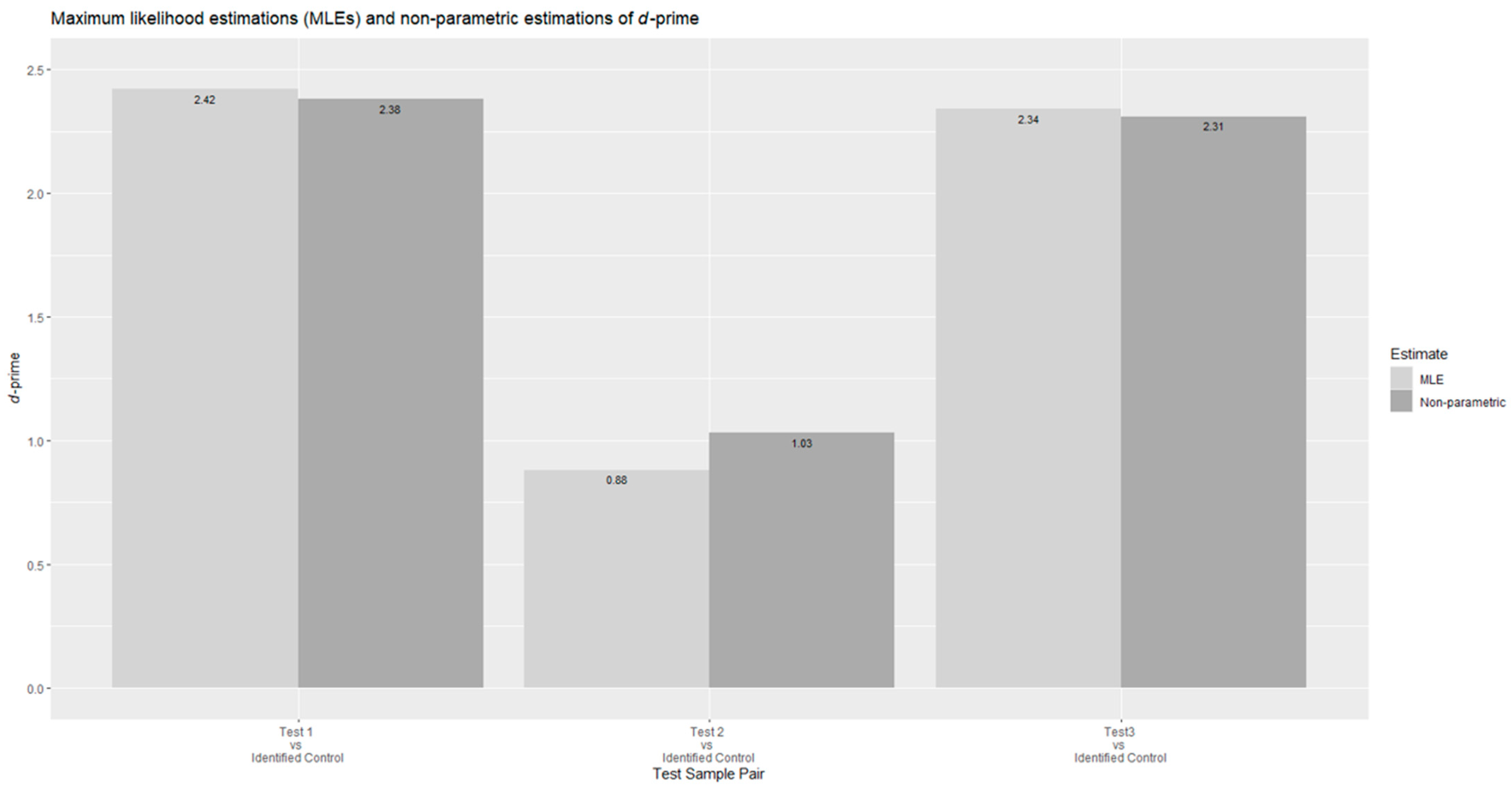
Figure 1 shows the d-prime values, i.e., the estimates of $\delta$ for three test samples vs. the identified control sample estimated by MLEs and nonparametric estimations. MLE and nonparametric estimation generally produce consistent and similar results. MLE is more popular and powerful with smaller estimation errors, while an advantage of nonparametric estimation is that there is no assumption for distributions. However, it is noted that the nonparametric estimation is, in fact, for the AUC. The d-prime is indirectly obtained from the AUC based on an area theorem.

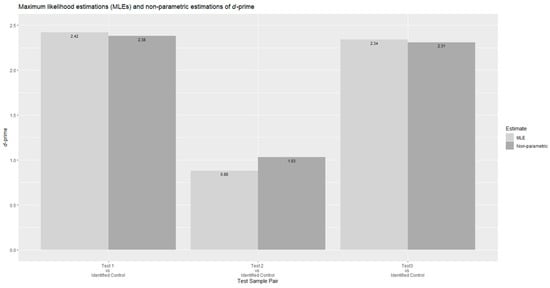
Figure 1. d-prime values estimated by MLEs and nonparametric estimation.

3.2. Statistical Tests for $\delta$, ${\delta }_f$, or $A_{dfc}$

The R codes for the statistical tests are provided in Bi and Kuesten [27]. The statistical tests are conducted in this section using the results of the estimators $\hat{\mathsf{\delta }}$ and their variances obtained in Section 3.1.1 (Table 3). The data file ‘alldp’ in R can be obtained by ’alldp<-DFCdps()’.

The same test procedures can be applied for testing ${\delta }_f$ or $A_{dfc}$ using the estimators of ${\delta }_f$ or $A_{dfc}$ and their variances. The differences are only that for the difference test for ${\delta }_f$, the null hypothesis is $H_0: {\delta }_f=$ 1.13; however, for the difference test for $A_{dfc}$, the null hypothesis is $H_0: A_{dfc}$ = 0.5.

3.2.1. Difference Test Based on Individual Parameters, e.g., d′ and Its Variance

The R code ‘dpdtest(d,v)’ can be used for the difference test with the null hypothesis $H_0: \delta =0$ and the alternative hypothesis $H_a: \delta >0$ based on an individual d′ value and its variance.

For example, the result of the difference test is as below for the data in the second row in the data file ‘alldp’: d′ = 0.88, and the variance of d′, i.e., var(d’) = 0.0390. A significant difference was found between test sample 2 and the control sample in the DFC test, with a p-value < 0.0001.

3.2.2. One-Sided Equivalence/Similarity Test Based on Individual Estimator, e.g., d′, Its Variance, and a Specified Similarity Limit

The R code ‘dpstest(d,v, slim)’ can be used for the one-sided equivalence/similarity test with the null hypothesis $H_0: \delta \ge {\Delta }_0$ and the alternative hypothesis $H_a: \delta <{\Delta }_0$ based on an individual d′ value, its variance, and a specified similarity limit ${\Delta }_0$. For example, the result of the equivalence/similarity test is as below for the data in the second row in the data file ‘alldp’: d′ = 0.88, var(d’) = 0.0390, and a specified similarity limit ${\Delta }_0$ = 1.5. Because the p-value < 0.01, significant equivalence/similarity between test sample 2 and the control sample can be claimed in terms of the equivalence/similarity limit ${\Delta }_0$ = 1.5 at a significance level $\alpha$ = 0.01. This means that the perceptual difference between test sample 2 and the control sample is smaller than the specified perceptual difference in terms of the Thurstonian discriminal distance d′ = 1.5.

3.2.3. Difference Test Based on Multiple Parameter Values, e.g., Multiple d′ Values and Their Variances

The R code ‘dstest (d, v)’ can be used to conduct a difference test with the null hypothesis $H_0: {\delta }_1={\delta }_2=\cdots ={\delta }_k$ and the alternative hypothesis $H_a: {\delta }_i\ne {\delta }_j, i.j=1,2,\dots k$, i.e., if significant, at least two parameters are different for multiple d′ values and their variances. For example, for the three d′ values and their variances in ‘alldp’ for the three test samples vs. the control sample, the test results can be obtained by ‘dstest(d=alldp[,1],v=alldp[,2])’. A significant difference was found among the three test samples in the DFC test, with a p-value < 0.01.

3.2.4. Multiple Comparisons for Multiple Parameter Values, e.g., Multiple d′ Values and Their Variances

The S-Plus program ‘multicomp(x,vmat,alpha)’ in S-PLUS 6.0 (Insightful [32]) can be used for the multiple comparisons, based on a vector of multiple d-prime (‘dp1’) and a co-variance matrix (‘dv1’) with a selected alpha level, e.g., alpha = 0.2. The input of the program includes x = dp1 (dp1<-alldp[,1]) and vmat=dv1 (dv1<-matrix(0,3,3), diag(dv1)<-alldp[,2]), with alpha = 0.2.

The R programs ‘confint’, ‘glht’, and ‘parm’ in the R package ‘multcomp’ Version 1.4-28 (Hothorn, et al. [33]) can also be used for the multiple comparisons, based on ‘dp1’ and ‘dv1’, with a selected confidence level (1-alpha), e.g., 0.8 (alpha = 0.2).

Significant differences were found between test sample 1 (T1) and test sample 2 (T2), and between test sample 2 (T2) and test sample 3 (T3).

3.2.5. Equivalence/Similarity Test Based on Two Parameter Values, e.g., Two d′ Values, Their Variances, and a Specified Similarity Limit

The R code ‘s2dptest(d,v,d0)’ can be used for the two one-sided tests (TOSTs) with the two sets of one-sided hypotheses $H_{01}:-{\Delta }_0 \ge {\delta }_1-{\delta }_2$ versus $H_{a1}:-{\Delta }_0<{\delta }_1-{\delta }_2$ and $H_{02}: {\delta }_1-{\delta }_2\ge {\Delta }_0$ versus $H_{a2}: {\delta }_1-{\delta }_2<{\Delta }_0$ for two test samples based on two estimators, e.g., $d^{{\prime }_1}$ and $d^{{\prime }_3}$ for test samples T1 and T3 and their variances. The input of the code is the two $d^{\prime }$ estimators and their variances, as well as an equivalence/similarity limit ${\Delta }_0$. The outputs of the code are the test statistics Z1 and Z2 and the p-values.

For example, for the data d = c(2.42,2.33), v = c(0.0203,0.0199), and an equivalence/similarity limit d0 = 0.5, the output is pv1 = 0.0016 and pv2 = 0.0204. Significant equivalence/similarity of T1 and T3 can be concluded with an equivalence/similarity limit of d0 = 0.5 at a significance level of $\alpha =$ 0.05.

3.3. Difference Testing Power and Sample Size for DFC Data in Terms of $A_{dfc}$

The R code ‘DFCpower(d,samp,alpha)’ can be used to calculate the difference testing power for the DFC test in terms of $A_{dfc}$. The input of the code includes a specified perceptual difference in terms of $\delta$ (d), sample size (samp), and a significance level (alpha). The output includes a corresponding $A_{dfc}$ and the testing power.

For example, for a specified difference (d = 1.2), sample size (samp = 100), and significance level (alpha = 0.1), the corresponding $A_{dfc}$ = 0.6 and the testing power is 0.78.

The R code ‘DFCsamp(d,pow,alpha)’ can be used to estimate the sample size needed for difference testing for the DFC test. The input of the code includes a specified perceptual difference in terms of $\delta$ (d), testing power (pow), and a significance level (alpha). The output includes a corresponding $A_{dfc}$ and sample size.

For example, for a specified difference (d = 1.2), testing power (pow = 0.8), and significance level (alpha = 0.1), the corresponding $A_{dfc}$ = 0.61 and the sample size is 93.

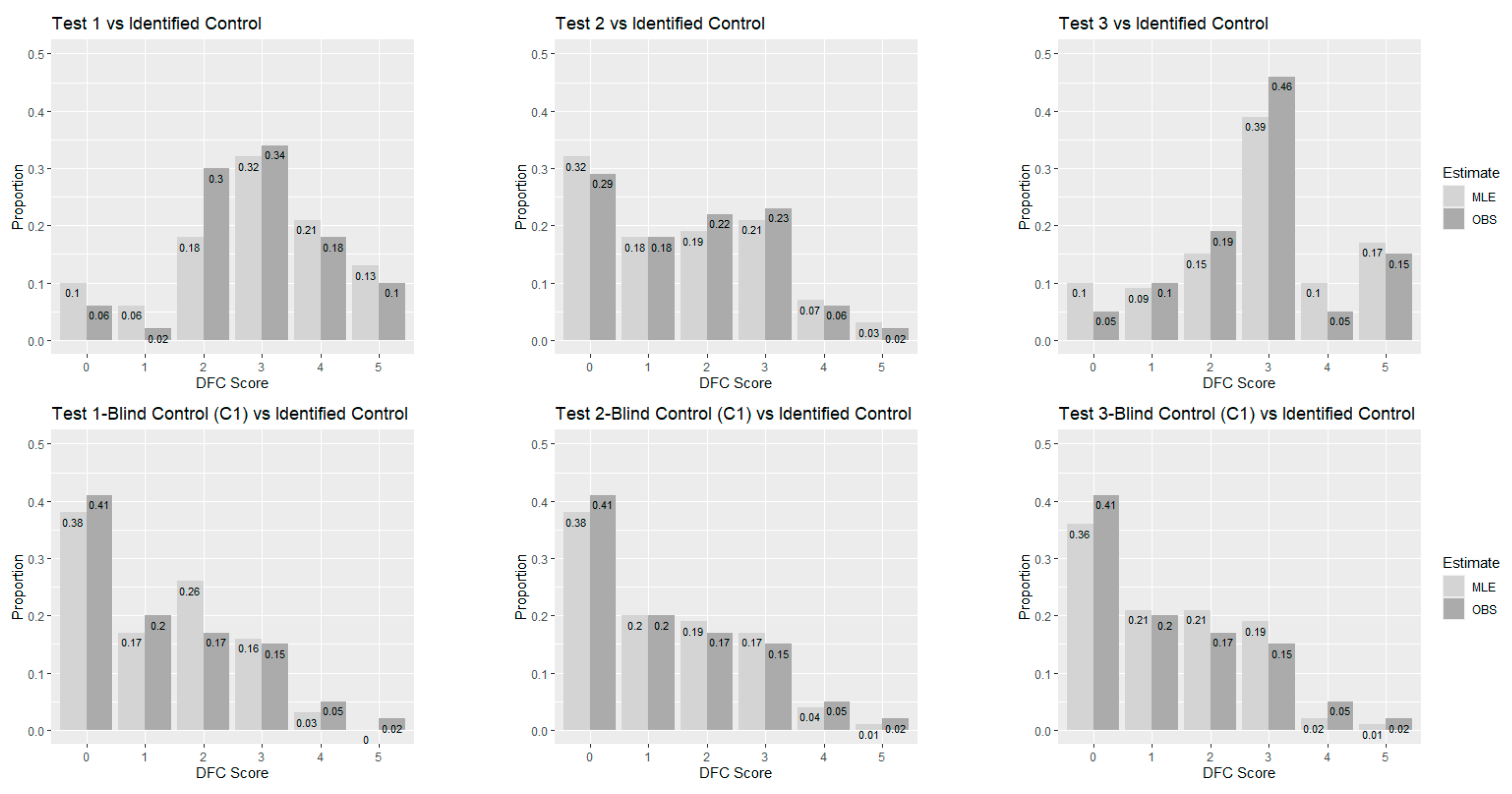
3.4. Observed Proportions and Predicted Probabilities for Categories of DFC Ratings

The R code ‘DFCmle0(x)’ can be used to produce predicted probabilities of the DFC categories of Hit (H) and False-alarm (FA) based on the observed proportions or frequencies of the DFC ratings and MLE results. For example, for the rating frequencies of the blind control vs. the identified control in the first column in the data file ‘dfc6’, and for the rating frequencies of test sample 1 vs. the identified control in the second column in the data file ‘dfc6’, the observed proportions of the DFC categories are as below.

>dfc6[,c(1,2)]/100
Blind Control	vs.	Identified Control Test 1	vs.	Identified Control
5		0.02		0.10
4		0.05		0.18
3		0.15		0.34
2		0.17		0.30
1		0.20		0.02
0		0.41		0.06

The predicted probabilities of the DFC categories are as below.

>DFCmle0(dfc6[,c(1,2)])
C1	vs.	C T	vs.	C
5		0.0043		0.1263
4		0.0290		0.2113
3		0.1582		0.3201
2		0.2647		0.1817
1		0.1660		0.0624
0		0.3777		0.0981

Figure 2 shows the observed proportions and predicted probabilities of the categories of the DFC ratings for three test samples vs. the identified control.

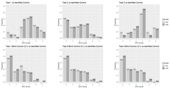
Figure 2. Observed proportions and predicted probabilities of the categories of the DFC ratings.

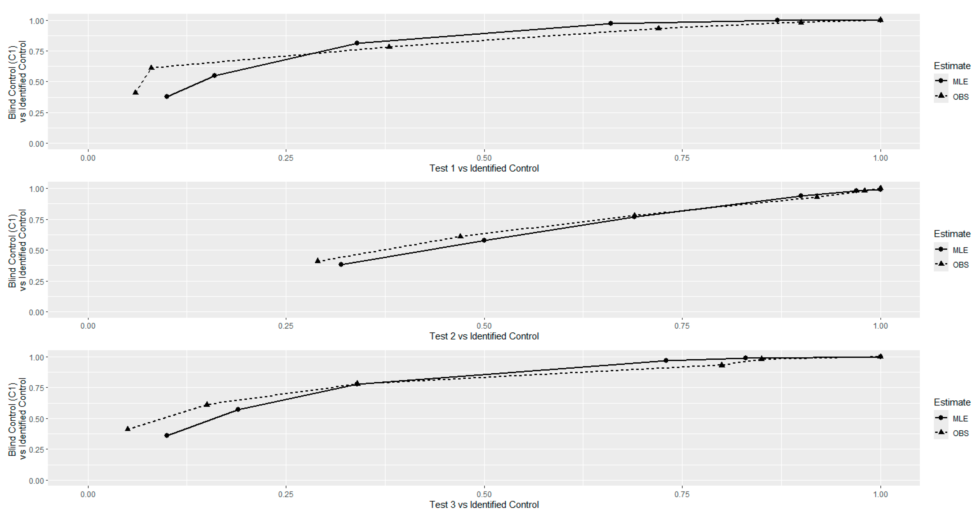
Figure 3 shows the corresponding ROC curves based on the proportions and probabilities shown in Figure 2.

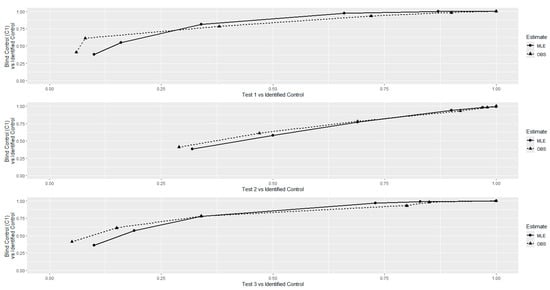
Figure 3. ROC curves based on the observed proportions and predicted probabilities for three test samples vs. the identified control.

Figure 2 and Figure 3 are visualizations of the comparisons of the observed proportions and predicted probabilities of the categories of the DFC ratings based on the folded normal distribution. Although the observed proportions and the predicted probabilities are not exactly the same, they are consistent and similar in general. This suggests that the model of the folded normal distribution is suitable for the DFC ratings data in general.

4. Discussion

4.1. Thurstonian Model for the DFC and the Ratings of the Same-Different Method

Although as one of the advanced and powerful sensory analysis tools, the Thurstonian model for sensory discrimination methods is not new in the sensory literature (see, e.g., ASTM [34]), the model for the specified sensory discrimination method, the DFC, has not been discussed adequately and used widely in the sensory field.

This paper originally derives the Thurstonian model for the DFC test and novelly demonstrates that the model is based on the folded normal distribution and is the same as that for the ratings of the Same-Different method. Although the two methods share the same Thurstonian model, the DFC is different from the ratings of the Same-Different method in the designs of the methodologies.

In the DFC test, assessors are provided with an identified control sample, followed by one or more test samples, including blind controls. The assessor’s task is to scale how different they perceive the test sample(s), including blind controls, to be from the identified control sample. In the DFC test, the only possible same sample pair is C/C1 and the only different sample pair is T/C, where T denotes the test sample, C denotes the control sample, and C1 denotes the blind control sample.

In the Same-Different test, two products of interest (A and B) are selected. It is not necessary for the two products to be a test sample and a control sample. Assessors are presented with one of the four possible sample pairs: A/A, B/B, A/B, or B/A. The assessor’s task is to categorize the given pair of samples as same or different (ASTM [34]). For the ratings of the Same-Different method, the assessor’s task is to give ratings for sureness of difference for any given sample pair.

Note that the Thurstonian model in the R program ‘dod’ in the R package ‘sensR’ Version 1.5-3 (Christensen, et al. [17]) is just the variant of the DOD for the ratings of the Same-Different method. Using the R program ‘dod’ in the R package ‘sensR’ and the data ‘dfc6’, the estimated d-prime is 2.391 with a standard error of 0.22211 (i.e., variance 0.2211² = 0.0489), which are consistent with the results (d-prime = 2.4168 with variance 0.0203) obtained by using the R code ‘DFCmle(x)’ in Section 3.1 of this paper.

4.2. Scales Used in the DFC Test

There are different types of scales used for DFC ratings. For the larger number of k in the k-point rating scales, the frequencies for some categories may be smaller or zero. It is suggested to coalesce the frequencies for larger numbers of the k-point scale into the frequencies in a smaller number of categories. For example, this would involve transferring the 100-point scale data or 9+1-point scale data into a six-point scale, or three-point or two-point scale data. In theory, the parameter $\delta$ is independent of the criteria. Hence, in theory, for a specified control sample and a specified test sample, the parameter $\delta$ should be unchanged by using different types of scales.

Note that the R codes ‘DFCmle (x)’ can be used for the MLE of parameters (indices) for k-point scale DFC data where k is larger than or equal to two. The DFC is the same as the Same-Different method when k is equal to two.

It is noted that the data ‘dfc3’ with a three-point rating scale in Table 5, and the data ‘dfc2’ with a two-point rating scale in Table 6 were summarized from the data ‘dfc6’ with a 6-point rating scale in Table 2. The ‘dfc3’ and ‘dfc2’ data can be produced by ‘dfc3<-DFC3ps()’ and ‘dfc2<-DFC2ps()’, where the R codes ‘DFC3ps()’ and ‘DFC2ps()’ can be found in the Supplementary Materials.

Table 5. Frequencies of ratings with a three-point scale in the DFC (data ‘dfc3’).

Categories *	Blind Control vs. Identified Control	Test Sample 1 vs. Identified Control	Test Sample 2 vs. Identified Control	Test Sample 3 vs. Identified Control
3	7	28	8	20
2	32	64	45	65
1	61	8	47	15

* Note: Degree of difference from control: 1 = “looks the same”, 2 = “not sure”, 3 = “looks different”.

Table 6. Frequencies of ratings with a two-point scale in the DFC (data ‘dfc2’).

Categories *	Blind Control vs. Identified Control	Test Sample 1 vs. Identified Control	Test Sample 2 vs. Identified Control	Test Sample 3 vs. Identified Control
1	22	62	31	66
0	78	38	69	34

* Note: Degree of difference from control: 0 = “same”, 1 = “different”.

The MLE results of the parameters (indices) $\delta$, ${\delta }_f$, and $A_{dfc}$ for the data files ‘dfc3’ and ‘dfc2’ are listed in Table 7 and Table 8. We can find that the estimated values for the three data files are similar and consistent.

Table 7. Maximum likelihood estimations (MLEs) of $\delta , {\delta }_f$, and $A_{dfc}$ for the three-point scale DFC data in Table 5.

	Test Sample 1 vs. Identified Control		Test Sample 2 vs. Identified Control		Test Sample 3 vs. Identified Control
	Value	Variance	Value	Variance	Value	Variance
$\hat{\delta }$ ($d^{\prime }$)	2.57	0.0482	0.85	0.0906	2.16	0.0467
$\widehat{{\delta }_f}$	2.60	0.0417	1.33	0.0185	2.24	0.0356
$\widehat{A_{dfc}}$	0.82	9 × 10−4	0.55	0.0013	0.76	0.0012

Table 8. Maximum likelihood estimations (MLEs) of $\delta , {\delta }_f$, and $A_{dfc}$ for the two-point scale DFC data in Table 6.

	Test Sample 1 vs. Identified Control		Test Sample 2 vs. Identified Control		Test Sample 3 vs. Identified Control
	Value	Variance	Value	Variance	Value	Variance
$\hat{\delta }$ ($d^{\prime }$)	2.16	0.0606	0.91	0.1167	2.31	0.0606
$\widehat{{\delta }_f}$	2.23	0.0462	1.35	0.0267	2.37	0.0488
$\widehat{A_{dfc}}$	0.76	0.0016	0.56	0.0018	0.78	0.0014

4.3. Qualifier and Limitation of the DFC Test

As one of the sensory discrimination methods, the DFC test is applicable to sensory evaluation in process optimization and quality assessment for foods. The DFC test is applied for specific situations where a reference control is available and the goal is to determine if a noticeable difference exists. The DFC test may be used for reformulation testing, process changes, ingredient substitutions, quality control, and batch consistency. The Thurstonian model provides some useful indices, including the Thurstonian discriminal distance $\delta$ or $d^{\prime }$, to measure the perceptual difference or similarity between a test sample and a control sample. An advantage of the index $\delta$ or $d^{\prime }$ is that it is independent of the methods and scales used. The use of the indices would influence decision-making in industrial applications or QA/QC procedures because these indices are more useful and reasonable than the conventional rating means. The indices are continuous scales, while the ratings scale in the DFC is not. This is why the Thurstonian model is necessary for every sensory discrimination method, including the DFC.

The DFC test is not appropriate when no control sample is available, understanding specific differences in depth is required, determining consumer acceptance or preference, optimizing sensory attributes, comparing multiple product variations at once (i.e., ranking test), or conducting exploratory testing with untrained panelists. The DFC test can be more variable, since panelists rate the degree of difference rather than simply identifying if a difference exists as is done for other discrimination tests (i.e., triangle, duo–trio, and tetrad tests). The DFC test may require a larger sample size to detect small differences reliably. It does not provide detailed profiling of sensory attributes.

4.4. Relevance of DFC for Sensory Evaluation Practices

The DFC is particularly useful to sensory researchers for product development, quality control, and shelf-life/storage stability studies. As a sensory evaluation technique that measures how much a sample deviates from a reference or “control” sample, it can be applied for ingredient substitution and flavor optimization, reformulation or process changes, routine screening, and pharmaceutical/palatability testing. DFC is used to assess overall or ‘holistic’ sensory perceptual difference from a control. Advantages of DFC include that it is rapid, simple, and efficient for data collection, based on a category or line scale, it is sensitive to small perceptual differences, the data are statistically analyzable, and the results are suitable for tracking gradual change. Limitations include that DFC results lack attribute-specific details (does not specify what changed), relies on a consistent control (any drift in the control undermines the method), and is less useful with untrained panels (due to the abstract nature of the “difference magnitude”). It is of interest to note that Compusense, Inc. offers a video showing execution of the DFC method on YouTube [35]. References for applications where DFC may be used are summarized below.

4.4.1. DFC Resources

• Product development (ingredient substitution and flavor optimization, reformulation, or process changes)

DFC is among the recommended methods to detect differences from standards during reformulation efforts [36]. Difference-from-control methods are featured in quality control and reformulation contexts [37] (pp. 121–123). Applied use of DFC is shared for plant-based proteins [38] and sodium reduction [39]. Meilgaard et al. [4] present coverage of DFC testing in product matching and ingredient change validations, and Whelan [7] presents DFC case studies.

• Quality control and routine screening

Details and guidelines for use of difference tests in QC and in–out attribute screening are available [36]. For an example of using a QC panel and a 10-point DFC scale where readings above a threshold indicate rejection, see King et al. [40]. Kilcast [41] also shows supportive use of DFC with examples for sensory quality control. ASTM [42] presents the DFC test method as an example of a “product-focused” scale for use in quality control (QC). The advantages include the following: DFC is a rapid approach to measuring the overall difference, is amenable to a threshold selection process (i.e., pass/fail based on a difference), and less training is required vs. a descriptive panel. Disadvantages include the following: DFC is no replacement for a detailed sensory profile, does not provide directional assessment (unipolar scale), and it may be difficult to calibrate a panel to rate differences. Another ASTM reference [43] covers DFC with an example and recommendations for DFC as a viable method for QC. This manual distinguishes differences in the DFC test from the DOD test based on how variance is handled. The DOD test differs from the DFC test in that the variance as a result of judging (as measured by reference versus blind-coded reference) is averaged with the variance as a result of the batch or lot of product. Further, this manual distinguishes an approach named as the difference from reference (DFR) test, which uses a reference sample, a set of test samples, and a blind-coded reference sample, which is used as the estimate of panel variance. Notably, care should be taken in deciding the approach for difference testing and how the data should be analyzed.

• Shelf-life studies

ASTM #2454-20 [44] outlines best practices for using DFC (often via a degree of difference scale) to detect sensory drift over time. Munoz [2] and [45] also provide further shelf-life study information and guidance for detecting sensory changes, endpoint criterion, and go-no-go screening for stability studies. Hough [46] (pp. 44–46) describes an example for applying the difference-from-control test (when the size of the difference is more important than simply knowing of the existence of a difference) using a cutoff methodology based on the size of differences in acceptability perceived by consumers, coupled with the corresponding size of the difference perceived by a trained panel. Additionally, Sharma et al. [47] provide further research examples for shelf-life evaluation methods and quality monitoring.

• Pharmaceutical/palatability studies

Clapham et al. [48] discuss sensory testing against appropriate controls, citing several useful ISO and ASTM documents, but is remiss in explicitly mentioning the DFC approach for tracking palatability and acceptability in drug products over time.

4.4.2. DFC Applications

Table 9 presents application areas, example scales tailored to each area based on the literature, and common, best practices with the DFC method. Typical scale types, category labels, and usages are listed. In addition, typical experimental designs used with DFC tests are shared by application area. These designs aim to ensure statistical power, control for variability, and maximize relevance to the sensory goals.

Table 9. Summary of difference-from-control (DFC) usages by application.

Application	Scale				Design
	Scale Example	Scale Type	Scale Category Labels	Usage	Typical	Samples	Panel Type	Goal
Product Development
-Reformulation and process change	Rate the overall difference from the standard product.	10-point labeled scale or line scale	0 = No difference 2 = Slight dif 5 = Moderate dif 7 = Strong dif 9 = Extreme dif	Can be used in pre-screening before full descriptive profiling or consumer testing	Randomized complete block design	Control: Original formula or process Test: Multiple reformulations or process variants	Trained or descriptive	Detect if reformulated products differ perceptibly from the control standard
-Ingredient substitution or flavor optimization	Evaluate the overall difference from the control.	10-point difference intensity scale	0 = No dif 1 = Barely detectable 3 = Mild 5 = Moderate 7 = Strong 9 = Very strong dif	Often paired with consumer Just-About-Right (JAR) or hedonic scales for product development	Randomized complete block or mixture design (if systematic substitution)	Control: Current formulation Test: Versions with partial or full ingredient substitution	Trained or semi-trained; target consumers for hedonics	Identify substitutes that minimize differences from control; test with systematized variation
Quality control (routine screening)	How different is this batch from the gold standard?	6- or 8-point scale, often with alert thresholds	0 = Identical 1 = Slight dif (acceptable) 3 = Noticeable difference (still acceptable) 5 = Clear difference (may need investigation 7 = Major deviation (not acceptable)	May include a pass/fail cutoff score (e.g., ≥4 triggers a review or hold)	Single sample vs. control (single trial or ongoing monitoring)	Control: Reference standard from a known acceptable batch Test: Daily/weekly production batch	Expert or trained internal panel	Flag batches that deviate from standard product; threshold-based (pass/fail)
Shelf-life and stability	How different is this sample from the fresh control?	Unstructured or 0–10-point line scale	0 = No difference 10 = Extremely different	Often used with a sensory change threshold (e.g., DFC ≥ 5 = “perceptible change”) for estimating shelf-life endpoints	Repeated measures or balanced incomplete block	Control: Fresh product (baseline) Test: Same product at multiple storage intervals	Trained or semi-trained	Track degree of change over time vs. fresh
Pharmaceutical/palatability	How different is this formulation compared to the control?	0–10-point line scale, with optional child-friendly wording	Example (adult): 0 = No difference in taste/mouthfeel 10 = Extremely different (unpleasant change in taste, texture, or aftertaste) Child: 5-face or emoji scale —Same —Slight dif —Big dif	Especially useful when masking bitter or metallic off-notes.	Paired comparison with DFC rating	Control: Original or masked formulation Test: New active drug formulation or flavor mask	Adults (trained) or caregiver/child proxy	Ensure palatability changes are minimal or acceptable; sensitive to small changes

4.4.3. DFC Database Schemas

Researchers may be interested in collecting DFC ratings on an ongoing basis. Databasing this information is useful and may require different metadata fields for each application area. For effective use of DFC data and building a powerful multi-study database, the following variables should be standardized: DFC scales, control samples, sensory descriptors (attributes), panelist demographics (where applicable), test protocol(s), and environmental/test conditions.

Table 10 below summarizes database schemas (data structures) to collect metadata and results for DFC tests across each application area, either by individual study or aggregated in multi-study databases for longitudinal or meta-analysis. Hypothetical research questions tailored to each application area are provided. The metadata can be used to achieve the following: (1) model shelf-life trends over time and different conditions, (2) link sensory changes to formulations/processes, (3) auto-trigger actions if DFC scores exceed selected threshold(s), (4) link variables to sensory acceptability trends, and (5) identify ingredient-performance thresholds using substitution(s) levels.

Table 10. Difference-from-control (DFC) data structures and research questions.

Application	Key Metadata Fields	Key Research Questions	Database Scalable Questions
Product Development
-Reformulation and process change	Sample ID Reformulation Code Panelist ID DFC Score Batch No Process Params Test Date Comments	- Does a new ingredient/process result in a perceptible difference compared to the original? - Which changes in formulation or processing variables most affect sensory perception? - How much change (e.g., % substitution) is acceptable before the product is perceived as different?	- Are certain types of reformulations (e.g., fat reduction or plant-based substitutions) more likely to exceed DFC rejection thresholds? - Which ingredient swaps repeatedly result in acceptable/no-difference outcomes? - Do trained panel DFC scores correlate with consumer hedonic outcomes across reformulations?
-Ingredient substitution or flavor optimization	Sample ID Ingredient Code Substitution Level (%) Panelist ID DFC Score Sensory Note Date Tested	- At which level of ingredient substitution does the product become perceptibly different? - Which sensory notes (e.g., bitterness or dryness) contribute most to differences? - Is a particular substitute consistently less detectable than others?	- What ingredient substitutions maintain DFC scores below rejection thresholds across product types? - Is there a pattern in how different protein/fat/sweetener substitutions affect DFC? - How does consumer liking correlate with DFC scores across substitution studies?
Quality control (routine screening)	Batch ID Panelist ID DFC Score Test Date Production Line Shift Alert Flag Corrective Action	- Does the production batch differ from the reference standard? - Are deviations in DFC scores correlated with machine/shift/operator data? - Can DFC scoring detect subtle sensory drift before instrumental measures do?	- What are acceptable DFC score limits for different product types and production lines? - How often do DFC-based alerts align with consumer complaints or off-spec issues? - Which operational variables (e.g., ingredient lot, supplier, or shift) predict higher DFC variability?
Shelf-life and stability	Sample ID Storage Time Days Panelist ID DFC Score Date Tested Storage Condition Notes	- At what storage duration do sensory changes become perceptible (DFC ≥ threshold)? - Which sensory attributes degrade first during storage, and at what rate? - Do different storage conditions (e.g., temperature, humidity, and light) affect the onset or degree of perceptible sensory changes? - Can DFC scores be used to predict consumer rejection points?	- How does sensory shelf-life vary by product category or formulation? - Is there a consistent relationship between DFC score trajectory and chemical spoilage (e.g., oxidation)? - Are there “critical thresholds” of DFC that consistently precede consumer drop-off?
Pharmaceutical/palatability	Formulation ID Subject ID Age Group DFC Score Masking Agent Flavor Used Test Date Adverse Comment	- Does a formulation with an active drug taste significantly different from its placebo? - Does the masking agent or flavor system reduce the perceived sensory difference? - Are differences more pronounced in certain demographic groups (e.g., children vs. adults)?	- Which active ingredients are consistently associated with high DFC scores (poor palatability)? - Which masking strategies most effectively reduce DFC scores across drug types? - Do DFC results correlate with compliance or acceptability outcomes in different populations?

4.4.4. DFC Training

Training is required for DFC testing. DFC asks panelists to quantify how different a sample is from a control—not in what ways it differs or if it is better. Training is needed to ensure consistency, scale calibration, and understanding of how to rate “magnitude of difference” on a unipolar scale. It can be difficult to calibrate a panel to rate differences. For these reasons, the DFC is not recommended with consumers due to ambiguity on how to apply the scale without training. Though DFC ratings can be collected from consumers, if so, the results should be interpreted with caution. A best practice for training a panel to use DFC involves several steps:

(1)

The DFC task is clarified by making sure panelists will compare each test sample against a fixed control, that they are not evaluating liking, direction, or attribute-specific intensity, and that their goal is to assess the overall perceived magnitude of difference. It is emphasized that 0 = no difference and the maximum point = most different imaginable.

(2)

The panel is trained with a product set designed to span the range of expected differences using anchored examples: 0 = no difference, 2–3 = slight difference, 5–6 = moderate difference, and 8–10 = strong difference.

(3)

The panel undergoes practice with feedback using a known control vs. modified samples, participates in debriefing and discussion after each test, and is shown the average group scores to highlight consistency (or variability). They are provided feedback on individual and group results, discuss differences in perception or scoring habits, and train for consistency, not conformity.

(4)

Scale interpretation is reinforced with visual or verbal anchors; printed guides may be considered, especially for newer panelists.

(5)

Ongoing monitoring and calibration is continued; using repeat blind duplicates to measure panelist consistency may be considered; and individual and group scores may be tracked to identify drift or outliers.

(6)

To improve sensitivity to small changes, even if the DFC scale remains ‘holistic’, panelists are pre-trained with individual attributes to boost perceptual awareness.

4.4.5. When Is DFC Appropriate vs. Alternatives?

The DFC test is popular for measuring sensory differences between test and control samples; however, it may not always be the best choice depending on the research objective(s), panel type, and regulatory need. Alternative discrimination methods (triangle test, tetrad test, duo–trio, and degree of difference (DOD)), descriptive analysis (DA), consumer testing (check-all-that-apply (CATA), rate-all-that-apply (RATA), and Just-About-Right (JAR)), temporal methods, or others may be more suitable. DFC is never appropriate when a control reference product is not available. When detailed profiling is needed, consider DA, the tetrad test, or RATA. For specific temporal changes, use descriptive analysis, just-noticeable-difference (JND), temporal dominance of sensations (TDS), or temporal RATA. For masking performance, try TDS, DA, or preference tests. When consumer difference testing results are needed for liking or emotions, consider using CATA, RATA, JAR, or hedonic scales, not DFC. Keep in mind specific scales may be required to satisfy legal claims.

5. Concluding Remarks

A Thurstonian model for the DFC test provides a useful index, $\delta$ or $d^{\prime }$, to measure the perceptual difference between test sample(s) and the identified control sample. This paper originally derives the Thurstonian model based on the folded normal distribution. It is demonstrated that the DFC, as a variant of the degree of difference (DOD) method, shares a common Thurstonian model with another variant of the DOD, i.e., the ratings of the Same-Different method, though the DFC and the ratings of the Same-Different are quite different sensory discrimination methods. Maximum likelihood estimates and nonparametric estimates of the parameters of the model are provided. Statistical tests, including different tests and equivalence/similarity tests for individual or multiple d’ values obtained from the DFC test, are also conducted in this paper.

References

- ISO 20613; Sensory Analysis—General Guidance for the Application of Sensory Analysis in Quality Control. ISO: Geneva, Switzerland, 2019. Available online: https://www.iso.org/standard/68549.html (accessed on 4 June 2025).
- Muñoz, A.M.; Civille, G.V.; Carr, B.T. Sensory Evaluation in Quality Control; Van Nostrand Reinhold: New York, NY, USA, 1992. [Google Scholar]
- Costell, E.A. Comparison of sensory methods in quality control. J. Food Qual. Prefer. 2002, 13, 341–353. [Google Scholar] [CrossRef]
- Meilgaard, M.; Civille, G.V.; Carr, B.T. Sensory Evaluation Techniques, 4th ed.; CRC Press: Boca Raton, FL, USA, 2007. [Google Scholar]
- Kemp, S.E.; Hollowood, T.; Hort, J. Sensory Evaluation: A Practical Handbook; Wiley-Blackwell: Oxford, UK, 2009. [Google Scholar]
- Lawless, H.T.; Heymann, H. Sensory Evaluation of Food: Principles and Practices, 2nd ed.; Springer: New York, NY, USA, 2010. [Google Scholar]
- Whelan, V.J. Difference from control (DFC) test. In Discrimination Testing in Sensory Science: A Practical Handbook; Rogers, L., Ed.; Elsevier: Amsterdam, The Netherlands; Woodhead Publishing: Duxford, UK, 2017. [Google Scholar]
- ASTM-E2262-03; Standard Practice for Estimating Thurstonian Discriminal Distances. ASTM International: West Conshohocken, PA, USA, 2021.
- Bradley, R.A. Comparison of Different-from-Control, Triangle, and Duo-Trio Tests in Tasting: Comparable Expected Performance; Memorandum Prepared for the General Foods Corporation; General Foods Corporation: Rye Brook, NY, USA, 12 November 1957. [Google Scholar]
- Bradley, R.A. Some relationship among sensory difference tests. Biometrics 1963, 19, 385–397. [Google Scholar] [CrossRef]
- Aust, L.B.; Gacula, M.C., Jr.; Beard, S.A.; Washam, R.W., II. Degree of difference test method in sensory evaluation of heterogeneous product types. J. Food Sci. 1985, 50, 511–513. [Google Scholar] [CrossRef]
- Bi, J. Statistical models for the Degree of Difference method. Food Qual. Prefer. 2002, 13, 31–37. [Google Scholar] [CrossRef]
- Bi, J.; Lee, H.S.; O’Mahony, M. Statistical analysis of ROC curves for the ratings of the A-Not A and the Same-Different methods. J. Sens. Stud. 2013, 28, 34–46. [Google Scholar] [CrossRef]
- Ennis, D.M.; Rousseau, B.A. Thurstonian model for the degree of difference protocol. J. Food Qual. Prefer. 2015, 41, 159–162. [Google Scholar] [CrossRef]
- Ennis, J.M.; Christenson, R.A. Thurstonian comparison of the Tetrad and Degree of Difference tests. J. Food Qual. Prefer. 2015, 40, 263–269. [Google Scholar] [CrossRef]
- Ennis, D.M. Thurstonian Models: Categorical Decision Making in the Presence of Noise; The Institute for Perception: Richmond, VA, USA, 2016; ISBN 9780990644606/099064460X. [Google Scholar]
- Christensen, R.H.B.; Brockhoff, B.P.; Kuznetsova, A.; Birot, S.; Stachlewska, K.A.; Rafacz, D. Package ‘sensR’. 2023. Available online: https://cran.r-project.org/web/packages/sensR/index.html (accessed on 1 July 2025).
- Bi, J. Sensory Discrimination Tests and Measurements: Sensometrics in Sensory Evaluation, 2nd ed.; Wiley/Blackwell Publishing: Oxford, UK, 2015. [Google Scholar]
- Read, C.B. Folded distributions. In Encyclopedia of Statistical Sciences; Kotz, S., Johnson, M.L., Eds.; John Wiley & Sons: West Sussex, UK, 1983; Volume 3. [Google Scholar]
- Leone, F.C.; Nelson, L.S.; Nottingham, R.B. The folded normal distribution. Technometrics 1961, 3, 543–550. [Google Scholar] [CrossRef]
- Elandt, R.C. The Folded Normal Distribution: Two Methods of Estimating Parameters from Moments. Technometrics 1961, 3, 551–562. [Google Scholar] [CrossRef]
- Johnson, N.L. The folded normal distribution: Accuracy of estimation by maximum likelihood. Technometrics 1962, 4, 249–256. [Google Scholar] [CrossRef]
- Tsagris, M.; Beneki, C.; Hassani, H. On the Folded Normal Distribution. Mathematics 2014, 2, 12–28. [Google Scholar] [CrossRef]
- Chatterjee, M.; Chakraborty, A.K. A simple algorithm for calculating values for folded normal distribution. J. Stat. Comput. Simul. 2016, 86, 293–305. [Google Scholar] [CrossRef]
- Kaplan, H.L.; Macmillan, N.A.; Creelman, C.D. Tables of d′ for variable-standard discrimination paradigms. Behav. Res. Methods Instrum. 1978, 10, 796–813. [Google Scholar] [CrossRef]
- Bi, J. Variance of d′ from the same–different method. Behav. Res. Methods Instrum. Comput. 2002, 34, 37–45. [Google Scholar] [CrossRef] [PubMed]
- Irwin, R.J.; Hautus, M.J.; Butcher, J.C. 1999. An area theorem for the Same–Different experiment. Percept. Psychophys. 1999, 61, 766–769. [Google Scholar] [CrossRef] [PubMed]
- Swets, J.A. Measuring the accuracy of diagnostic systems. Science 1988, 240, 1285–1293. [Google Scholar] [CrossRef] [PubMed]
- R Core Team. R: A Language and Environment for Statistical Computing, version R 4.5.0; R Foundation for Statistical Computing: Vienna, Austria, 2023; Available online: https://www.R-project.org/ (accessed on 19 June 2025).
- Gilbert, P.; Varadhan, R. Accurate Numerical Derivatives R Package “numDeriv”. 2019. Available online: https://cran.r-project.org/web/packages/numDeriv/index.html (accessed on 29 June 2025).
- Bi, J.; Kuesten, C. Thurstonian Scaling for Sensory Discrimination Methods. Appl. Sci. 2025, 15, 991. [Google Scholar] [CrossRef]
- Insightful. S-PLUS 6. In Guide to Statistics Vol.1. for Windows; Insightful Corporation: Seattle, WA, USA, 2001. [Google Scholar]
- Hothorn, T.; Bretz, F.; Westfall, P.; Heiberger, R.M.; Schuetzenmeister, A.; Scheibe, S. R Package “multcomp”: Simultaneous Inference in General Parametric Models. 2023. Available online: https://cran.r-project.org/web/packages/multcomp/index.html (accessed on 29 June 2025).
- ASTM-E2139-05; Standard Test Method for Same-Different Test. ASTM International: West Conshohocken, PA, USA, 2018.
- Making Sense of: Difference from Control (DFC). Video Posted on YouTube. Available online: https://www.bing.com/videos/riverview/relatedvideo?q=E253-09+Standard+Practice+for+Sensory+Evaluation+of+Products+by+a+Difference-from-Control-Method&qpvt=E253-09+Standard+Practice+for+Sensory+Evaluation+of+Products+by+a+Difference-from-Control-Method&view=riverview&mmscn=mtsc&mid=22DB11E992B22B7A17CC22DB11E992B22B7A17CC&&aps=201&FORM=VMSOVR (accessed on 12 June 2025).
- Carpenter, R.P.; Lyon, D.H.; Hasdell, T.A. Guidelines for Sensory Analysis in Food Product Development and Quality Control, 2nd ed.; Springer: New York, NY, USA, 2000. [Google Scholar]
- Meilgaard, M.C.; Civille, G.V.; Carr, B.T.; Osdoba, E.T. Sensory Evaluation Techniques, 6th ed.; CRC Press: Boca Raton, FL, USA, 2025. [Google Scholar]
- Bowen, A.; Blake, A. Lessons for the Sensory Characterization of Plant-Based Proteins. SSP Presentation. 2024. Available online: https://www.sensorysociety.org/meetings/archives/2024Conference/Documents/04%20Bowen_SSP.pdf#search=DFC (accessed on 12 June 2025).
- Leong, J.; Kasamatsu, C.; Ong, E.; Hoi, J.T.; Loong, M.N. A study on sensory properties of sodium reduction and replacement in Asian food using difference-from-control test. Food Sci. Nutr. 2015, 4, 469–478. [Google Scholar] [CrossRef]
- King, S.; Gillette, M.; Titman, D.; Adams, J.; Ridgely, M. The Sensory Quality System: A global quality control solution. Food Qual. Prefer. 2002, 13, 385–395. [Google Scholar] [CrossRef]
- Kilcast, D. (Ed.) Sensory Analysis for Food and Beverage Quality Control: A Practical Guide; Woodhead Publishing Limited: Cambridge, UK, 2010. [Google Scholar]
- E3041-17(2025); Standard Guide for Selecting and Using Scales for Sensory Evaluation. ASTM International: West Conshohocken, PA, USA, 2025.
- MNL14-2ND-EB; The Role of Sensory Analysis in Quality Control. 2nd ed. Ojeh, S., Ed.; ASTM International: West Conshohocken, PA, USA, 2021.
- E2454-20; Standard Guide for Sensory Evaluation Methods to Determine Sensory Shelf Life of Consumer Products. ASTM International: West Conshohocken, PA, USA, 2020.
- Sensory Shelf-Life Test Edited by M. Johnson. SSP. 2021. Available online: https://www.sensorysociety.org/knowledge/sspwiki/Pages/Sensory%20Shelf-Life%20Test.aspx (accessed on 12 June 2025).
- Hough, G. Sensory Shelf Life Estimation of Food Products; CRC Press: Boca Raton, FL, USA, 2010. [Google Scholar]
- Sharma, C.; Torrico, D.D.; Singh, S. Chapter: Sensory Methods for Shelf Life Assessment of Foods. In Shelf Life and Food Safety, 1st ed.; CRC Press: Boca Raton, FL, USA, 2022; pp. 33–60. [Google Scholar]
- Clapham, D.; Belissa, E.; Inghelbrecht, S.; Pensé-Lhéritier, A.M.; Ruiz, F.; Sheehan, L.; Shine, M.; Vallet, T.; Walsh, J.; Tuleu, C. A Guide to Best Practice in Sensory Analysis of Pharmaceutical Formulations. Pharmaceutics 2023, 15, 2319. [Google Scholar] [CrossRef] [PubMed] [PubMed Central]
Disclaimer/Publisher’s Note: The statements, opinions and data contained in all publications are solely those of the individual author(s) and contributor(s) and not of MDPI and/or the editor(s). MDPI and/or the editor(s) disclaim responsibility for any injury to people or property resulting from any ideas, methods, instructions or products referred to in the content. |
© 2025 by the authors. Licensee MDPI, Basel, Switzerland. This article is an open access article distributed under the terms and conditions of the Creative Commons Attribution (CC BY) license (https://creativecommons.org/licenses/by/4.0/).