Abstract
The sustainable utilization of forest biomass for bioenergy production is increasingly challenged by the variability and unpredictability of raw material availability. These challenges are particularly critical in regions like Central Portugal, where seasonality, dispersed resources, and wildfire prevention policies disrupt procurement planning. This study investigates two flexibility strategies—dynamic network reconfiguration and operations postponement—as policy relevant tools to enhance resilience in forest-to-bioenergy supply chains. A novel mathematical model, the mobile Facility Location Problem with dynamic Operations Assignment (mFLP-dOA), is proposed and solved using a scalable matheuristic approach. Applying the model to a real case study, we demonstrate that incorporating temporary intermediate nodes and adaptable processing schedules can reduce costs by up to 17% while improving operational responsiveness and reducing non-productive machine time. The findings offer strategic insights for policymakers, biomass operators, and regional planners aiming to design more adaptive and cost-effective biomass supply systems, particularly under environmental risk scenarios such as summer operation bans. This work supports evidence-based planning and investment in flexible logistics infrastructure for cleaner and more resilient bioenergy supply chains.
1. Introduction
In recent years, research into risk management has been increasing, particularly in supply chains that explore natural resources. Unexpected supply interruptions impact the overall process of these supply chains, resulting in lost sales and poor financial performance [1]. In forest-based supply chains, managing risk and variability in the procurement stage is crucial and affects downstream decisions related to logistics, inventory management, and production planning [2,3].
Chopra and Sodhi [2] highlight the frequent sources of risk and variability associated with the procurement stage, which cause delays or shortages of raw materials. These disruptions result from a high capacity utilization at a supply source, the high percentage of raw materials procured from a single source, and the inaccurate forecasts of the delivery amounts. Usually, this is a consequence of seasonality, long lead times, a and wide variety of products. In forest-to-bioenergy supply chains, variability primarily stems from the difficulty in accurately predicting the location, timing, and quantity of raw material availability within a given period [4,5,6].
The forest-to-bioenergy supply chain involves a network of supply nodes where chippers—equipment used to convert forest residues into biomass—are deployed to carry out processing operations. The resulting biomass is then transported by truck to designated delivery nodes. Many of these supply sites present operational challenges: they are often difficult to access, require extensive setup and site preparation, and offer limited and heterogeneous quantities of raw material. Additionally, some sites are located in more productive regions than others [7]. Chipping operations are further influenced by site-specific conditions, seasonal weather patterns, and the timing of forest harvesting activities throughout the year [8,9]. This combination of spatial and temporal uncertainty in raw material availability complicates supply chain planning, underscoring the need for strategies that mitigate variability in the procurement process [5,6].
Among the different techniques to mitigate variability, supply chain flexibility is a quick solution with inexpensive implementation costs, and is described by Sánchez and Pérez [10] as the ability to change or react to diversity and uncertainty with a minor penalty in time, effort, cost or performance, and can improve the competitiveness of the company.
Some authors have already addressed the challenge of introducing more flexibility into the planning of biomass logistics operations. The researches of Gunnarsson et al. [11], Silva et al. [12], Piqueiro et al. [8], and Gautam et al. [13] propose mathematical models to incorporate decisions related to the quantity of biomass to store at intermediate nodes. Moreover, Ng and Maravelias [14] respond to this challenge, suggesting a pre-processing of agriculture-based biomass in intermediate nodes. This biomass is densified into pellets before being delivered to conversion facilities. The review of essential features and new trends in biomass logistics by Malladi and Sowlati [15] reveals a lack of studies about operations planning models that combine dynamic network reconfiguration with operations postponement.
In light of the observed gaps in current literature and practice, this study is guided by the following research questions: (1) Under what conditions does the integration of dynamic network reconfiguration and operations postponement improve the performance of forest-to-bioenergy supply chains? (2) How can these flexibility strategies be optimally combined within a mathematical framework to reduce the negative impacts of procurement variability? (3) What are the operational trade-offs and computational implications of implementing these strategies in real-world scenarios characterized by spatial and temporal uncertainty? These questions direct the development of our modeling approach and computational experiments, aiming to generate insights that are both theoretically grounded and practically relevant.
This work considers two flexibility strategies: (1) dynamic network reconfiguration and (2) operations postponement, to adapt supply chain design and operations along time according to current resource availability, achieving economies of scale and reducing operational costs.
The dynamic network reconfiguration consists of opening and closing temporary intermediate nodes over the time horizon (e.g., Sanci and Daskin [16]), adjusting the number and location of these storage nodes to the availability of raw material. This first flexibility strategy can be combined with the strategy of postponing operations from supply to intermediate nodes to cope with temporal variability of raw material supply (e.g., Jabbarzadeh et al. [17]). Figure 1 represents our problem in the logistics network design of the forest-to-bioenergy supply chain. In the figure’s left side (a), this process occurs without any flexibility strategy, and in the right side (b), the process is depicted after the adoption of the previous two flexibility strategies.
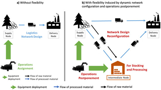
Figure 1.
Representation of logistics network design of forest-to-bioenergy supply chain.
The main contributions of this paper are threefold. Firstly, we introduce a mobile Facility Location Problem including Dynamic Operations Assignment (mFLP-dOA) to map the forest-to-bioenergy supply chain presented before. Consequently, we propose a new Mixed-Integer Programming (MIP) model to provide solutions to this problem and explore the advantages provided by two flexibility strategies: (1) dynamic network reconfiguration and (2) operations postponement. Secondly, we devise a matheuristic procedure to solve the MIP model, obtaining good quality solutions for large instances generated from a case study within a reasonable computational time. Finally, we are the first to perform extensive computational experiments combining the two flexibility strategies in different risk scenarios to understand under which conditions these strategies are most valuable.
The remainder of this paper is organized as follows. Section 2 provides a review of the literature regarding flexibility strategies and optimization techniques for dynamic network reconfiguration with postponement decisions that allow us to place our work in context. Section 3 presents the mathematical formulation to address flexibility in procurement planning. Section 4 describes the solution approach developed, which is based on a fix-and-optimize algorithm. Section 5 presents the computational experiments performed in different risk scenarios with close-to-reality instances from a forest-to-bioenergy supply chain in Portugal. The main conclusions and discussion are presented in Section 6.
2. Literature Review
To address the research questions outlined in the Introduction section, our study investigates the adoption of flexibility strategies aimed at mitigating the risks associated with variability in raw material availability during the procurement process. Specifically, we explore the effectiveness of two strategies, dynamic network reconfiguration and operations postponement, under different risk scenarios. This review also informed the selection of relevant optimization techniques for dynamic network reconfiguration, which are essential for implementing our proposed solution framework. The resulting model is formulated as a mobile Facility Location Problem with dynamic Operations Assignment (mFLP-dOA), enabling the evaluation of the proposed flexibility strategies in response to spatial and temporal uncertainty in supply conditions.
2.1. Strategies to Enhance Flexibility in the Supply Chain
Tang and Tomlin [18] identified five flexibility strategies covering the different stages of the chain. The first, flexible supply via multiple suppliers, consists of shifting order quantities across suppliers to create redundancy in supply fulfillment and overcome the risk of unresponsive suppliers. The second, flexible supply via flexible supply contracts, consists of shifting order quantities across time to deal with the risk of production breakdown due to the seasonality in the availability of raw materials. The third, flexible manufacturing, consists of shifting production quantities across internal resources. The fourth, operations postponement, consists of delaying the time when an activity or task is performed. The fifth, responsive pricing, consists of shifting demand across different products to deal with the uncertainty and variability in customers’ demand.
There are some recent studies with the application of some of these flexibility strategies proposed by Tang and Tomlin [18]. Saghiri and Barnes [19] studied the possibility of postponement of the downstream supply chain activities related with shipping and final product configuration (for example, labeling, packaging, or assembly). Wong et al. [20] showed that significant cost savings are achievable by postponing the labeling and packaging processes until current orders from retailers are known. These savings include the reduction of the cycle, safety, and obsolete stocks. They also show that the estimated potential benefits of this flexibility strategy are greater than the costs associated with reconfiguration.
Kamalahmadi and Parast [21] studied flexible supply via multiple suppliers and compare it with two other strategies: strategic stock that consists of defining safety inventory levels for raw materials, works-in progress, and finished products along the nodes of the supply chain; and facility fortification that consists of reinforcing key facilities and related infrastructures to better resist to a natural hazard such as a flood or fire. The authors concluded that all three strategies reduce costs and risks compared to the solution without flexibility and that adding redundancy to the supply chain in different forms with contingency plans can help companies mitigate the impact of supply chain disruptions.
There is a lack of research to analyze the impact of network flexibility in model development and practical decision-making in supply chain network design [22]. Network flexibility is usually implemented at the operational planning level. However, recent research has revealed that network flexibility may significantly impact location decisions and should, thus, be considered holistically in the network design [23].
Darvish et al. [24] and Vahid Nooraie and Parast [25] studied a flexibility strategy, called dynamic network reconfiguration, where new facilities may be opened along time, hence adjusting the capacity to the variability in respect to supply and demand fluctuations. Darvish et al. [24] combined flexibility in network design through the location of temporary intermediate nodes, with another type of strategy, flexible service time to customers, leading to cost savings of up to 30%. Sanci and Daskin [16] also studied dynamic network reconfiguration to deal with the risk of disasters that damage roads and other city infrastructures in Istanbul.
One of the listed flexibility strategies that seemed most promising for the forest-to-bioenergy supply chain was dynamic network reconfiguration. This strategy allows dealing with variability in raw materials availability in forest-to-bioenergy supply chains, adapting the network configuration to the availability of raw materials. Opening and closing intermediate stockyards between the forest sites and the bioenergy plants enable freight consolidation, transportation costs and ensure regular wood flows. Consequently, an additional strategy that leverages the establishment of intermediate nodes involves postponing biomass pre-processing from the extraction sites to these intermediate nodes, which can lead to economies of scale and reduction in operational costs.
There are few examples in the supply chain management literature that quantify the impact of different flexibility strategies in different risk scenarios. The findings of our study enrich the literature by providing an in-depth understanding of these two strategies and how to combine and implement them to mitigate different levels of variability.
2.2. Implementing Dynamic Network Reconfiguration and Operation Postponement Strategies
Simulation, optimization, and other quantitative methods are often used to implement and perform comparative analysis, but there are few examples of the application of combined flexibility strategies in quantitative assessments. Examples of quantitative methods appear in several applications such as textiles and clothing [26,27], manufacturing and automotives [10,28], and food supply chains [29], in which are a comparison of several firm performance indicators when different flexibility strategies are implemented.
One of the examples of quantitative analysis with different flexibility strategies combined is given by Hammami and Frein [30], who proposed a model for dynamic network reconfiguration combined with another flexibility strategy, transfer pricing, for the automotive industry. Indeed, companies can use transfer pricing to shift profits to lower-tax countries (e.g., on the relocation of operations and manufacturing facilities). This strategy has a direct impact on network reconfiguration decisions.
The dynamic network reconfiguration strategy is usually modeled as a facility location problem, and Table 1 presents some examples of this application and implementation. Cortinhal et al. [31] also developed a model for dynamic network reconfiguration, which integrates location and capacity choices for plants and warehouses with supplier and transportation mode selection as well as outsourcing options over multiple periods.
Darvish et al. [24] applied a Flexible Two-Echelon Location Routing Problem (FLRP-2E) to study the possibility of changing the location of temporary intermediate nodes in combination with flexible service times to customers. The model is instrumental for computing the cost savings concerning different risk scenarios. Similar Two-Echelon Location Problems are addressed by Ortiz-Astorquiza et al. [32] and Rohaninejad et al. [33].
Vahid Nooraie and Parast [25] developed a multi-objective stochastic model and analyzed trade-offs between the investment costs of opening facilities and the supply chain risk exposure. Torabi et al. [34] combined dynamic network reconfiguration with multiple suppliers and strategic stock in the context of humanitarian organizations. They propose a two-stage scenario-based mixed fuzzy stochastic programming model that combines decisions related to which supplier to select, stock levels, and opening central or local warehouses, tested in different pre-disaster and post-disaster scenarios. In a similar setting, Sanci and Daskin [16] proposed a two-stage stochastic programming model that combines decisions related to the location of the temporary disaster recovery locations and the restoration equipment that should be assigned to them. Yu and Solvang [23] provided a new fuzzy-stochastic multi-objective model to simultaneously deal with multiple objectives, different types of uncertainty, and network flexibility in closed-loop supply chain network design.
Based on the analysis of the literature review (see Table 1), our study adopts a mobile facility location problem to addresses the decisions related to opening and closing intermediate nodes along the planning horizon for storage and eventually processing. Our model is multi-period and is based on a Two-Echelon Facility Location Problem to select which intermediate nodes to open in each period. Similar models can be found in Badri et al. [35], Halper et al. [36], and Raghavan et al. [37].
Our model copes with the decisions of postponing operations to these intermediate nodes (and moving equipment there), using a similar approach to de Keizer et al. [38], who propose a model for redesigning the European distribution network of flowers considering product quality decay and its heterogeneity. Biomass has similar problems to flowers as quality decreases over time. Results suggest higher profits from the use of four hubs for flower distribution and processing when compared with the current single hub in the Netherlands. The main difference concerning the work of de Keizer et al. [38] is that in the model they developed, they are allocating processes to different nodes (hubs) of the supply chain. In contrast to this research, we are considering a multi-period model that assigns specific operations to given equipment, locations, and periods, allowing us to quantify the duration of each operation in each node. Monthly tactical decisions related to dynamic network reconfiguration co-exist with daily chipping equipment reallocation/operations postponing decisions. Similar integrated models can be found in Akhtari et al. [39] and Badri et al. [35] to integrate strategic and tactical decisions for forest-based supply chains.
Table 1 presents more examples of implementing the postponement strategy to mitigate the variability present in supply chain planning. Jabbarzadeh et al. [17] formulate an integrated production-distribution planning model to respond to the uncertainty of pharmaceutical supply chain demand. They present a robust bi-objective optimization model for the integrated production and distribution of a supply chain with the postponement strategy. The two objectives are economic (cost minimization) and environmental (greenhouse gas emissions minimization). They find that the postponement strategy can consistently provide cost savings for the supply chain independent of greenhouse gas emissions and degree of demand variability.
Budiman and Rau [40] developed a two-stage stochastic model of a supply chain network (SCN) design integrated with postponement and modularization concepts. The proposed research considers multi-period and multi-product facility allocation planning involving procurement, processing, and sales. The speculation-postponement strategy (SP) optimizes the forecast-driven operations planning and service level of multiple products to adjust to global demand uncertainty and regional differences factors. The results also highlight the importance of configuring the SCN and SP strategy altogether to prevent sub-optimal solutions, such as the significant offset of the expected performance when the service level is not adjusted to demand uncertainty, showing how forecast-driven planning inaccuracy can be costly. This integrated approach proves to be an effective solution to mitigate global demand uncertainty risks. Following the same logic, Weskamp et al. [41] also developed a two-stage stochastic mixed-integer linear programming model applied in a case study from a company in the apparel industry, which comprises an integrated production and distribution planning approach, and considers postponement concepts to support the decision-maker under demand uncertainty.

Table 1.
Flexibility strategies and FLP extensions under study and related works in the literature.
Table 1.
Flexibility strategies and FLP extensions under study and related works in the literature.
| Reference | Flexibility | FLP Extensions | Solution Methods | |||||||||
|---|---|---|---|---|---|---|---|---|---|---|---|---|
| DNR | OP | MP | OA | ME | m | MS | Exacts | Heuristics | ||||
| Hinojosa et al. [42] | • | • | • | |||||||||
| Badri et al. [35] | • | • | • | • | • | • | ||||||
| Hammami and Frein [30] | • | • | • | • | • | |||||||
| Cortinhal et al. [31] | • | • | • | • | • | |||||||
| Halper et al. [36] | • | • | • | • | ||||||||
| Vahid Nooraie and Parast [25] | • | • | • | • | ||||||||
| de Keizer et al. [38] | • | • | • | • | • | |||||||
| Akhtari et al. [39] | • | • | • | • | ||||||||
| Rohaninejad et al. [33] | • | • | • | |||||||||
| Torabi et al. [34] | • | • | • | |||||||||
| Chauhan et al. [43] | • | • | ||||||||||
| Darvish et al. [24] | • | • | • | • | • | |||||||
| Jabbarzadeh et al. [17] | • | • | • | • | ||||||||
| Raghavan et al. [37] | • | • | • | • | ||||||||
| Sanci and Daskin [16] | • | • | • | • | ||||||||
| Weskamp et al. [41] | • | • | • | • | • | |||||||
| Yu and Solvang [23] | • | • | • | • | ||||||||
| Budiman and Rau [40] | • | • | • | • | • | |||||||
| Our problem | • | • | • | • | • | • | • | • | ||||
Legend: DNR (dynamic network reconfiguration), OP (operations postponement), MP (multi-period), OA (operations assignment), ME (multi-echelon), m (mobile), MS (multi-scale).
In terms of solution methods, it is possible to find in the literature several examples of exact methods and metaheuristics used to solve facility location problems more efficiently. Sanci and Daskin [16] and Yu and Solvang [23] use a sample average approximation (SAA) method to reduce the scenario set to a manageable size and the concentration sets to limit the number of first-stage decision variables, which reduce the problem size even further. Other authors apply relaxation methods, Badri et al. [35] and Hinojosa et al. [42] presented a Lagrangian Relaxation (LR) method and Vahid Nooraie and Parast [25] used a heuristic algorithm based on the relaxation method (satisfied constraints method). Halper et al. [36] presented a local search metaheuristic, while Chauhan et al. [43] a three-stage heuristic (3SH), which was based on decomposition and local exchange principles and involves a facility location and allocation problem, multiple knapsack subproblems, and a final local random search stage.
The high implementation cost of network design reconfiguration decisions highlights the importance of accurate decision-making. Therefore, using exact solution methods to solve these problems is more efficient than solutions with minor errors [44]. Some authors such as Akhtari et al. [39], Cortinhal et al. [31], de Keizer et al. [38], and Hammami and Frein [30] presented exact methods to solve the problem. Darvish et al. [24] developed a branch-and-bound algorithm, and Raghavan et al. [37] compared a branch-and-price algorithm with a local search. Rohaninejad et al. [33] and Khatami et al. [44] opted for a Benders’ decomposition algorithm, in which the problem is divided into a master problem with binary variables and other sub-problems with continuous variables. In our problem it is not feasible to apply this method because we have binary variables related to the opening of intermediate nodes in a master problem. However, we also have binary variables related to the allocation of equipment in the sub-problem.
Once the solver finds a feasible solution relatively quickly, we thought of using a matheuristic to take advantage of the initial solution obtained by the solver. Helber and Sahling [45], Karimi Dastjerd and Ertogral [46], and Chen [47] used a fix-and-optimize approach to solve lot-sizing problems. This method consists of a sequence of mixed-integer programs (MIPs) solved over all real-valued decision variables and a subset of binary setup variables. The solution of binary variables is a fixed parameter for the next MIPs that optimize other binary variables. The optimization of the algebraic decision model is done within the MIP solver and, therefore, the approach is flexible. The user can change the number of binary variables to be treated within a single MIP and the number of iterations in which these are optimized and fixed again, making the trade-off between solution time and solution quality [45]. We select an approach based on the study by Neves-Moreira et al. [48], an improvement matheuristic based on a Fix and Optimize scheme, capable of exploring the solution space of large problems, which are intractable for the best general-purpose solvers available. The algorithm is tested on some combinations of case study instances and validated with real-world instances belonging to the forest-to-bioenergy supply chain case study.
3. Modeling Approach
This section outlines the modeling approach to the problem to include all the necessary aspects to obtain a realistic solution to this supply chain’s logistical and operational costs. In addition to the mathematical formulation of the proposed model, this section describes different flexibility strategies adopted for supply chain planning and how the model was simplified for each of these strategies.
3.1. Combining Flexibility Strategies
There are several possible combinations of the flexibility strategies discussed earlier. If we consider two axes of flexibility, we have on the one hand (1) dynamic network reconfiguration related to spatial flexibility, and on the other hand (2) postponement operations linked to temporal flexibility. On the axis of spatial flexibility, we have three levels of flexibility: without intermediate nodes, with permanent intermediate nodes, and with temporary intermediate nodes, both for storage. We can combine this flexibility axis with the temporal flexibility axis, which is also split into three levels of flexibility related to the moment when operations can occur: on a first level, operations only occur in supply nodes, on a second level, the operations only occur in intermediate nodes, and at a third level, operations can happen in both nodes.
In this paper we focus on the combinations A, B, and C that will be the combinations to be implemented and compared in different risk scenarios in Section 5.
- Without Intermediate Nodes (A): in this option there is no possibility to open intermediate nodes. Consequently, all operations are performed on supply nodes.
- Processing only in Permanent Intermediate Nodes (B): this option implies that operations are performed only on permanent intermediate nodes, which only have a processing function.
- Processing in Supply and Temporary Intermediate Nodes (C): this option represents the highest level of flexibility studied, processing can be done on both nodes, and temporary intermediate nodes have storage and/or a processing function.
These combinations allow us to evaluate the solutions with lower (A) and higher (C) levels of flexibility and even an intermediate solution (B) that has been discussed and implemented in the field in some specific business cases. Only options A, B, and C, are selected to avoid redundancies in comparing the different combinations of the two flexibility strategies since similar options do not bring significant differences in evaluating different risk scenarios.
The mathematical formulation of the proposed flexible planning model to implement the different flexibility strategies to be studied is presented below.
3.2. Mobile Facility Location Problem Including Dynamic Operations Assignment (mFLP-dOA)
Our modeling approach is based on a facility location problem. We select a set of supply nodes to meet the demand of delivery nodes and include a new echelon in this network, intermediate nodes, which can store processed material from supply nodes. The model includes decisions such as where to process (supply nodes or intermediate nodes), when to process, for how long, and which equipment is allocated to perform these operations.
The developed model provides a set of daily plans with the allocation of teams and equipment available to the several supply nodes to process the raw material needed to satisfy the monthly orders from the delivery nodes. These daily plans provide the number of hours worked by each team and equipment, the flows of processed and unprocessed material, and stock decision variables that guarantee the conservation of flows over the time horizon.
In addition to the parameters related to these short-term decisions, there are parameters with a monthly time scale (periods), such as the availability of the material in supply nodes, the demand in delivery nodes, and the possibility of opening intermediate nodes. The short-term decisions are integrated into medium-term decisions to ensure model feasibility. We adopted two-time scales, months and days, to have these two decision levels in the same model.
The mathematical formulation of the mixed integer programming (MIP) model for the mobile Facility Location Problem including Dynamic Operations Assignment (mFLP-dOA) is now presented. The decision variables, sets, and parameters are presented first, followed by the objective function and the model constraints.
Some parameters used in this formulation are transversal to any business and others are specific of forest biomass supply chain. Trucks with unchipped material cannot carry the same load weight because unchipped material occupies three times more volume than chipped material, resulting in the use of the measurement conversion parameter . There are some parameters that vary across the planning horizon; the quantity available in the pile is becoming available throughout the timeperiods and the demand also varies during planning horizon.
Decision variables and the model are more comprehensive and can easily be adapted to other supply chains.
The objective function minimizes total costs. This is decomposed by Equations (1a)–(1c) which correspond to the costs of transporting processed and unprocessed material between the different nodes. Equation (1d) corresponds to the monthly cost of keeping the intermediate nodes open. Equation (1e) corresponds to the cost of deploying the equipment in a given location. Finally, Equation (1f) concerns the minimization of processing costs, which depend on the working hours of each piece of equipment.
subjected to:
Our model consists of a facility location problem (FLP), in which we select a set of supply nodes to be used to meet the demand of delivery nodes. For this purpose we have to ensure that the following constraints are fulfilled: flow leaving supply nodes cannot exceed its availability (constraint (2)), capacity (constraint (3)) at intermediate nodes, demand satisfaction (constraint (4)), ensuring that the flow from processing nodes in each timeperiod meets the demand of delivery nodes in that timeperiod.
We also have constraints related to the equipment assignment. We cannot have the same chipper allocated to two or more locations on the same day (microperiod) (constraint (5)), and we cannot have more than one chipper on the same supply node at the same time (constraint (6)). There is only flow of processed material from a supply node to another node when there is an equipment in this supply node (constraint (7)), and there is only flow of processed material in intermediate node from an intermediate node to a delivery node when equipment is present in this intermediate node (constraint (8)). The number of processing hours is upper bounded by the duration of the microperiod (day) working time (constraints (11), and (12)) and there is a reduction in the working time available in the microperiods in which deployments occur due to machines’ transport, loading, unloading, and set up times. The number of processing hours of specific equipment in a supply node is higher or equal to its processing productivity of raw material (constraint (13)), conversion ratio results from productivity losses related to slope, quantity of material, and location access. Constraints (14) and (15) ensure that there is only one deployment in a given microperiod when a chipper is moved to a different location where it was allocated in the previous microperiod.
Constraint (16) together with constraints (9) and (10) account for the possibility of open an intermediate node. If we have flows from an intermediate node and/or equipment allocated there, this intermediate node must be open. If there is no intermediate node open in a given timeperiod , then there will be no equipment allocation , nor flow , for this entire timeperiod. Constraints (17)–(22) assure the flow conservation via stock constraints. Constraint (23) ensures that at the end of the planning horizon, all raw material available in a given supply node will have to be removed, that is, transported to a destination node (processed or unprocessed). Finally, constraints (24) and (25) determine the domain of the decision variables.
The same model is used for combination options (A), (B), and (C) with some simplifications. We manipulate the type of postponement strategy to be used (processing only in supply nodes, intermediate nodes, and both), and we also restrict the possible arcs for each strategy.
For option (A) we restrict processing to supply nodes and there is only a flow of processed material from the supply nodes to the delivery nodes.
The model can be simplified for option (B) by adding constraint (26), responsible for fixing the intermediates nodes. This constraint ensures that whenever an intermediate node opens, it has to remain open until the end of planning horizon. In addition to this constraint, we limit the number of intermediate nodes to just one and force all operations to occur on intermediate nodes. There is no flow of processed material from the supply nodes to the delivery nodes.
4. Solution Approach
The mathematical formulation proposed for the problem can be solved by general-purpose solvers only when the size of the instances does not go beyond few locations, machines, and timeperiods. Note that for medium and large instances, the number of variables and constraints in the formulation renders the problem intractable. For that reason, we propose a matheuristic approach based on the ideas of the fix-and-optimize proposed by Sahling et al. [49] and the Variable MIP Neighborhood Search (VMNS) presented by Larrain et al. [50], which follows predefined variable decomposition strategies to iteratively solve a series of tractable subproblems to improve the solutions to a large problem. This approach has been applied successfully in multiple large and realistic problems [48,51,52]. In the following subsections, we first detail the variable decomposition strategies that are used during our matheuristic approach and then we detail how these strategies are intertwined to achieve an efficient approach.
4.1. Decomposition Strategies
A decomposition is a subset of decision variables that is selected to find local improvements, maintaining the remaining variables fixed. The proposed solution approach focuses on small subsets of decisions at a time using the formulation proposed in Section 3. Consider the entire set of integer variables in the formulation. Each subproblem is defined by selecting a subset of decision variables to be re-optimized. The remaining variables are fixed with the values obtained in the incumbent solution. Hence, a subproblem Model-Sub can be stated as follows:
Model-Sub: minimize objective function (1a)–(1f) subject to constraints (2)–(25) and the additional constraints:
where , , and , are values coming from the incumbent solution.
The subset is based on dimensions related to the problem on hand, such as machines, locations, and timeperiods. These dimensions are identified by a decomposition . Note that in each decomposition there is a trade-off between computational complexity and the potential for finding improvements. Therefore, the set of decomposition strategies needs to explore subsets of variables that are diverse in their composition (exploration) and size (intensification). The set of decomposition strategies considered in the proposed matheuristic approach is built based on three types of decompositions:
- Period-based decomposition consists on selecting all the integer variables referring to a single macroperiod.
- Entities-based decomposition consists on randomly selecting the integer variables referring to a subset of timeperiods, locations, and machines.
- Random-based decomposition consists on randomly selecting a subset of integer variables (i.e., 25%, 50%, or 75% of all variables).
Figure 2 provides a visual representation of the considered decomposition strategies.
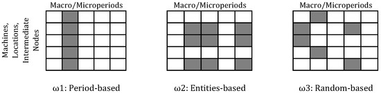
Figure 2.
Set of decomposition strategies considered in the matheuristic.
4.2. Matheuristic Procedure
The proposed matheuristic procedure is composed of two phases. The first phase focuses on finding a feasible integer solution by means of a relax-and-fix procedure. The second phase, a fix-and-optimize procedure, searches for solution improvements by solving a set of subproblems, focusing on smaller subsets of decisions. Both phases take advantage from the decomposition strategies described in Section 4.1 and from the versatility offered by general-purpose solvers. The following subsections detail the two phases of the proposed matheuristic procedure.
4.2.1. Relax-and-Fix
To build an initial solution, a relax-and-fix procedure is implemented. This procedure starts by relaxing the integrality constraints for all binary variables x, z, and y. These variables are converted to continuous variables. The next step consists of iteratively solving one subproblem for each macroperiod and its corresponding microperiods , thus, using a period-based decomposition approach. In each iteration, the variables x, z, and y referring only to the macro and micro periods of the current iteration are reconverted to binary variables. The MIP subproblem is solved with a time limit of and the values of the integer variable in the solution are saved so that they can be used in the next iterations to fix the integer variables of the periods already considered in previous iterations. After a subproblem is solved and its integer variables are fixed, the procedure advances to the next iteration to consider the next macroperiod. The procedure ends when all the integer variables are fixed and an initial solution is obtained. The detailed pseudo-code of this procedure is presented in Algorithm 1.
| Algorithm 1 Relax-and-fix outline |
|
4.2.2. Fix-and-Optimize
To improve the initial solution, a fix-and-optimize procedure is employed. This procedure is based on the decomposition strategies presented in Section 4.1. While the stopping criteria are not met, the iterative improvement procedure continues. In each iteration, a decomposition strategy is randomly selected and a subproblem considering the variables in the corresponding subset of variables is solved with a time limit of . If the incumbent solution improves, the best solution is updated. The cyclic procedure finishes when a certain number of non-improvements or a certain maximum time limit are achieved. The detailed pseudo-code of this procedure is presented in Algorithm 2.
| Algorithm 2 Fix-and-optimize outline |
|
5. Computational Experiments
The proposed approach is applied in a case study in the biomass-for-bioenergy supply chain in Central Portugal. The mathematical model is implemented in Gurobi 9.0 commercial solver. The solution method is developed in Python 3.6. The model is also used to compare the flexible supply chain planning strategies. A set of experiments are drawn to provide valuable managerial insights for planners about the impact of each flexibility strategy in different risk scenarios.
5.1. Case Study
The focal entity under study is a biomass provider company operating in the biomass-for-bioenergy supply chain in Central Portugal. The company is responsible for forest residues pre-processing and transporting the resultant wood chips up to the bioenergy plants to fulfill expected deliveries. The company agrees with each central operating in the region a minimum amount of wood chips to be delivered yearly. However, the expected daily deliveries are revised with a bit of advance. The company also establishes sourcing agreements with forest owners for collecting the forest residues that are the surplus of their forest harvesting operations. The region is dominated by Eucalyptus plantations which are harvested for pulpwood production in rotation cycles of 12 to 15 years. Forest residues correspond to the leaves, branches, and bark that are removed from the logs. This material is forwarded from the harvesting sites and piled in the vicinity of the forest roadside, separately from the pulpwood pile. The piles are geographically dispersed as there are several simultaneous harvesting sites in a region. There is seasonality of forest operations, concentrated between March and November to avoid rainier periods. Piles become available when harvesting is concluded. The company owns chippers and trucks and employs its specialized operators. Therefore, the company performs “longer-term” procurement planning to define which woodpiles to be expected and contracted in the next few months, hence establishing the expected flows to fulfill the bioenergy plants’ annual demand. Consequently, the company’s “short-term” planning consists of assigning and scheduling its workforce for the next few days at a minimum cost.
The company’s historical data was instrumental in characterizing the piles handled along with the 9-month planning (location, expected volume, when it is become available), the bioenergy plants (location, contracted weekly deliveries), and fleet (number of chippers, number of trucks, productivity of the chippers, truck freight, team working hours). Hence, the current supply chain configuration is composed of 52 piles of wood chips (supply nodes) and three bioenergy plants (demand nodes) (Figure 3).
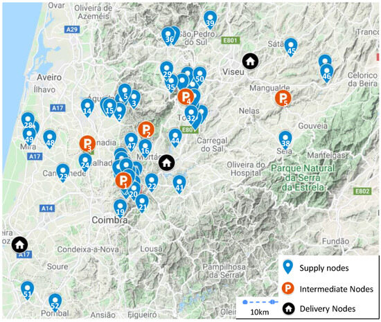
Figure 3.
Logistics network representation on map.
Intermediate stockyards are often not used. However, there are locations available at negligible costs. Hence, it is interesting to analyze if a reconfiguration of this network, including these temporary stockyards that can be opened and closed as needed, can help to reduce costs and better react to the variability in biomass availability. Currently, there are two chippers available with a productivity of 20 bulk cubic meters/hour of forest residues. Each chipper is assigned to an available pile and remains there until all forest residues are chipped. The transport of the resultant wood chips can start simultaneously with the chipping activities. The procurement plan considers nine months, each with 24 days (micro-periods), corresponding to 8 working hours. Overtime work is also possible but with an extra hourly cost.
The availability of raw material for all piles in the 9 month planning horizon is approximately 40,000 tons, the storage capacity for each intermediate node is 10,000 tons, and we have a total of 37,075 tons of demand. The unit of measurement selected was the ton because it facilitated the logistics operator’s supply and demand records. Based on the information provided by the company, we were able to estimate a productivity conversion ratio of 0.75. This ratio represents the biomass provider’s real productivity on the ground, compared to the productivity of the chipper working continuously in an intermediate node. The productivity losses due to the difficulty accessing the piles, areas with a very steep slope also hamper operations, limited availability of forest residues, and the forwarder’s productivity that directly influences chipper productivity.
We also consider that the conversion ratio of the transport capacity of a truck with unprocessed material is 0.3, meaning that chippers occupy, on average, three times less volume than unchipped forest residues. The transport capacity of a truck with processed material is 25 tons, and the truck distance cost is 1.2 EUR/km. Finally, the hourly operating cost for each machine was estimated at 170 EUR/h based on consumption, two operators for the machine, the average annual cost of damage, and insurance.
To simplify the model, we only consider a deployment cost. This assumption results from the interaction with different logistic operators who considered that the machines’ loading, unloading, and set up costs and the cost of preparing the location to receive the chipper (deforestation and road preparation operations) are the most significant. The cost of deploying the chipper for a location is EUR 250, taking into account the transportation cost based on an average distance between locations. We also defined an average percentage of lost working time in a deployment with these specialists, which is approximately 40% of daily working time.
In order to compare the performance of the solution method proposed, we generate a set of combinations of some parameters from the baseline instance to test our matheuristic, by varying some parameters, such as the number of supply nodes, number of intermediate nodes, number of delivery nodes and number of months in the planning horizon (see Table 2). Instances generated have different degrees of complexity with several numbers of decision variables.
Table 2.
Instance data set description. All the combinations between the parameters values in the table are generated.
5.2. Experiments Design
The pile’s potential location and the moment when the pile will become available are foreseen in the harvesting plans set yearly, and the biomass provider is informally informed. However, delays in the conclusion of the forest operations are common for several reasons, such as the machinery productivity being lower than expected due to site and weather conditions, machinery failures, and mandatory operation stoppages due to a higher fire risk. Based on the experts’ judgments, we assume that the piles expected during the hot season (June to September) are more likely to be delayed by one month on average. The number of forest residues can also be empirically estimated as a percentage of the total volume harvested. For eucalyptus plantations, forest residues correspond approximately to 40% of the harvested volume [12], which in turn can be approximated by historical data from previous harvests in the region. However, there are often deviations between the estimates and the actual volume collected due to the intrinsic difficulty of obtaining accurate yield and growth estimates and lack of visibility of the percentage of forest residues that ends up being incorporated in the soil to maintain site productivity conditions. Based on the experts’ judgments, we assume that the current piles’ volume may vary, reaching an increase of 20% of the initial estimate.
Accordingly, four main risk scenarios are defined:
- The optimistic scenario (baseline): corresponding to the baseline without incorporating variability in raw materials availability;
- Scenario (1): considers volumes more than 20% than the expected for all piles;
- Scenario (2): considers expected delays in all piles, resulting from the prohibition of any forestry operations during the month of August, as a preventive measure for fires;
- Scenario (3): results from the combination of the two previous scenarios, being the most pessimistic scenario.
For each option (A, B, and C) previously presented, the disruption caused by one of the risk scenarios is simulated. The experiments that test the adequacy of these combined flexibility strategies are driven by a deterministic approach.
Our design experiments start with the evaluation of each option in an optimistic scenario. To test the other scenarios, we run the model with the optimistic scenario (baseline) up to a certain period (end of macro period T = 05 ). After this moment, a replanning process is launched with a new parameter value entry (see Figure 4). After replanning, raw material availability, demand values, and the months available to allocate teams and equipment to carry out the operations are updated. The end of May is the period chosen for replanning because there is a closer estimate of the actual availability of raw materials and the dates of interruption of forest operations during the summer.
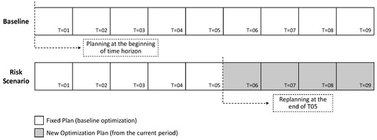
Figure 4.
Description of the replanning process applied in risk scenarios.
5.3. Results Analysis
The computational experiments in this paper aim at evaluating the performance of the proposed solution method and provide insights on the flexible procurement planning options to be adopted in different raw material variability scenarios.
5.3.1. Solution Method Results
Table 3 presents the performance of the solution method. The first four columns indicate the dimensions of the problem, namely, the number of months, supply nodes, intermediate nodes, and delivery nodes. Columns five to seven present the objective function, runtime, and the relative gap of the solutions obtained by the general-purpose solver. Columns 8 and 9 present the objective function and the runtime of the matheuristic. Finally, the last column shows the relative gap of the solution obtained by the matheuristic using the best non-integer solution found by the solver.
Table 3.
Comparison between the general-purpose solver and the matheuristic approach (MH).
Test runs are carried out for the same instances with the same runtime to compare the fix-and-optimize solution with the mathematical solver. The results show that as the complexity of the problem increases, the proposed solution method presents better performances, achieving the best objective function values more frequently. On average, the total cost achieved by the matheuristic is substantially lower than the one obtained by the solver across all instances. The proposed solution method improves the average optimality gap by 1.79 p.p. using shorter runtimes. Therefore, the results suggest that the proposed solution method is efficient and competitive against the considered general-purpose solver.
5.3.2. Results of Experiments Performed
Table 4 presents the results of the experiments carried out to test the efficiency of combinations of flexibility strategies in different risk scenarios. It can be concluded that the supply chain adapts better and with a lower cost of reconfiguring the network design when there is a month without operations than when there is an increase in the amount of biomass to process.
Table 4.
Presentation of the results of the combined flexibility strategies A, B and C in the different risk scenarios addressed.
Option (C) reached the lowest cost solution in all risk scenarios of the three flexibility strategies studied. This flexibility option adapts the network design, allowing us to open intermediate nodes close to supply nodes with greater availability in a given period, causing a large concentration of raw material in a given intermediate node in a given period, gaining economies of scale. On the other hand, the freedom to perform operations on both nodes allows us to allocate machines to intermediate nodes to gain productive efficiency and at the same time have machines allocated to dispersed supply nodes, in which it would not be profitable to open a new intermediate node or even transport the raw material to an existing intermediate node.
The graphical representation of each option allows us to understand the true impact of flexibility on daily decisions. Each of these options will constrain the movement of the machines, which has a very significant impact on the determination of flows and the respective operating costs. Figure 5 and Figure 6 represent the network design configuration of two combinations of flexibility strategies for two working days. In these figures, we can see different paths of the machines depending on the option selected, and the respective material flows for micro periods ( and ) belonging to July.
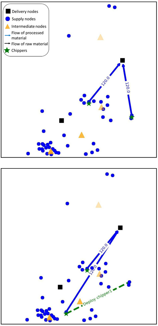
Figure 5.
Representation of optimized solution (option A) in period 07 (day 12 and 13).
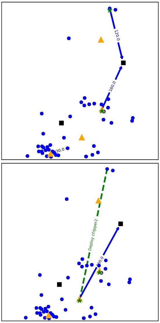
Figure 6.
Representation of flexible planning solution (option C) in period 07 (day 12 and 13).
In Figure 5, it is possible to observe that there is only a flow of supply nodes to delivery nodes. In Figure 6, it is interesting to note that there is a deployment of a chipper from a supply node to an intermediate node, demonstrating the flexibility of the model. On the first day shown in the figure (), only one intermediate node is being used, while on the following day (), two intermediate nodes are already being used. This versatility of the proposed model makes the entire supply chain more responsive and adaptable to the variability of raw material availability.
Table 5 and Table 6 present indicators that explain the difference in option solution values. All solutions presented for these under consideration scenarios were solved to optimality (Gap = 0).
Table 5.
Indicators of the results for optimistic scenario of the case study.
Table 6.
Indicators of the results for pessimist scenario of the case study.
For the pessimistic scenario, option C presents an efficiency gain of 16.39% compared to option A, much higher than the savings costs for the optimistic scenario, which were only 5.20%. The efficiency gain can explain this difference in values in the productivity of machines at intermediate nodes. As in the most pessimistic scenario (C3), we have an increase in raw material available to process in less available periods, and there is an agglomeration of material to process, resulting in an economy of scale.
Although option B can reduce deployments only for two, this decrease in deployment cost is not reflected in the same proportion in total cost since raw material transportation costs are high. Raw material takes up three times as much volume as processed material. There is a trade-off between optimizing the raw material transport cost and the productivity gains in postponing operations for intermediate nodes.
Table 6, contrary to what happens in the optimistic scenario, shows high values of overtime work. Option A has three times more overtime than the other two options, which can be explained by the efficiency gain in machine productivity when deployed on intermediate nodes. Option B has overtime work values similar to option C but does not have the same saving costs. This difference results from the cost of transporting the raw material, which for option B has to be transported to the same intermediate node. In contrast, for option C, as we can see in the table that there is an average of 2.44 intermediate nodes open per period that adjusts to the locations and availability of raw material in the supply nodes, minimizing the cost of transporting raw material.
6. Conclusions, Discussion and Future Work
The main objective of this research was to evaluate how the integration of multiple flexibility strategies (dynamic network reconfiguration and operations postponement) can improve procurement planning under spatial and temporal variability in raw material availability within forest-to-bioenergy supply chains. To address this objective, the study investigates flexible procurement planning strategies aimed at mitigating risks in the procurement process, such as inaccurate supply forecasts, dispersed and seasonal availability of supply nodes, and operational downtimes. The selected flexibility strategies were identified through a review of the literature on supply chain flexibility and tested in different risk scenarios to assess their effectiveness in improving adaptability and reducing costs.
While prior research, including that by Darvish et al. [24], Sanci and Daskin [16], and Vahid Nooraie and Parast [25], has quantitatively evaluated the benefits of dynamic network reconfiguration in response to supply risks, few works have simultaneously assessed the joint impact of multiple flexibility strategies under varying risk scenarios. Our study addresses this gap by proposing a mobile Facility Location Problem with dynamic Operations Assignment (mFLP-dOA), which integrates network reconfiguration with operations postponement in a multi-period setting.
While existing models in the literature have successfully explored flexibility strategies through classical optimization techniques, they often relied on assumptions or formulations that limit their applicability under highly variable and constraint-intensive environments like forest-based biomass supply chains. Approaches such as Benders’ decomposition (used by Rohaninejad et al. [33] and Khatami et al. [44]) are well suited to problems where binary variables are confined to the master problem and continuous ones to sub-problems. However, our model features binary decisions not only for the opening of intermediate nodes but also for the allocation of equipment within sub-problems, rendering such decomposition inapplicable. This structural complexity reflects the real-world need to simultaneously plan long-term infrastructure deployment and short-term operations reallocation, especially critical in fragmented forest landscapes with seasonal bans on summer operations. To address this modeling challenge, we adopt a mataheuristic based on the fix-and-optimize approach, as in Neves-Moreira et al. [48]. This flexibility is essential for managing the highly uncertain, seasonal, and geographically scattered nature of biomass supply. The ability to reallocate chipping equipment in response to evolving supply conditions while optimizing node openings allows for dynamic adaptation that is not captured in more rigid formulations.
Three different combinations of flexibility strategies were tested in an experimental design that evaluated the trade-off between the investment costs in intermediate nodes and the efficiency gains resulting from the opening of intermediate nodes in different risk scenarios. Option A represents the solution that does not incorporate any flexibility strategy, and option B admits the opening of a permanent intermediate node, and all operations occur there. Option C presents the possibility of open temporary intermediate nodes, and operations can occur in supply and intermediate nodes.
The results of this work indicate that adopting option (C), including temporary intermediate nodes for stocking and/or processing, leads to a cost reduction in all risk scenarios, especially for the pessimistic scenario, in which we have cost savings of 16.39%. Option (B) has smaller overtime than option (A) due to the productivity gains of migrating operations to the intermediate node, which does not result in efficiency gains because transporting all the raw material to a single intermediate node is very expensive. Since the volume of raw material transported is three times higher than that of the transport of processed material, the efficiency gain in this procurement process lies in the trade-off between the cost of transporting raw material and the productivity gains in intermediate nodes, which result in a reduction in the number of deployments and non-productive hours.
Our findings offer valuable guidance for stakeholders involved in forest biomass supply chains. For regional forest managers and biomass suppliers, the model provides a decision-support tool to optimize the timing and location of procurement and processing, enabling cost-effective use of temporary infrastructure under variable conditions. For policymakers, the results highlight the need for regulatory frameworks and infrastructure investments that support flexible and mobile supply chain configurations. These configurations are especially critical in adapting to seasonal constraints such as wildfire risk and weather conditions. By integrating logistics with landscape-scale risk management, our approach supports more resilient, sustainable, and regionally responsive bioenergy strategies.
This work contributes to the literature by studying the impact of combining different flexibility strategies in procurement planning for dealing with the variability in the availability of raw materials in forest-to-bioenergy supply chains. This study was validated using real-world data derived from a case study involving a biomass supplier operating within the biomass-for-bioenergy supply chain in Central Portugal. While the case study is based in central Portugal, the proposed model is adaptable to other European contexts with similar decentralized forest structures and seasonal operational constraints, though legal, climatic, and policy-specific adjustments may be required to reflect national biomass sourcing regulations and forest risk management frameworks. The developed matheuristic proved to be a suitable approach to tackle this problem, and this fact reiterated the interest of fix-and-optimize to solve facility location problems.
However, the model has some limitations that should be acknowledged. Even with the implementation of temporary stockyards to enhance network flexibility, the quality of stored biomass can degrade over time due to exposure to environmental conditions such as humidity, precipitation, and temperature variation—factors known to accelerate biomass deterioration, especially in open storage conditions. Additionally, intermediate storage may increase the risk of fire outbreaks in high-risk zones, particularly during the dry summer months, thus, interacting negatively with seasonal restrictions such as the summer ban on operations. The model assumes chipping as the primary pre-processing strategy, as aligned with the practices observed in the case study. However, recent operational trends show a shift toward baling, which can offer advantages in terms of logistics, storage stability, and moisture control. Incorporating these emerging technologies into the model could yield more robust and context-relevant planning tools.
One direction for future work concerns the modeling of other flexibility strategies applied to the case study, such as strategic stock positioning, modular processing infrastructure, or supplier diversification [18,21]. These strategies could be layered into the existing model structure to assess their combinatorial effects under different risk scenarios. Another direction for future work is introducing uncertainty factors in the problem through robust or stochastic optimization. Similar modeling efforts in other sectors, such as the two-stage stochastic programs used in disaster logistics [16,34] or the fuzzy-stochastic models applied to closed-loop supply chains [23], demonstrate the potential of such techniques to improve resilience in highly variable environments.
Author Contributions
R.G. was responsible for the model development, implementation, results, and original draft preparation. A.M. was responsible for conceptualization, reviewing, and editing. F.N.-M. was responsible for the methodology, implementation, and editing. C.A.N. and R.G.S. were responsible for reviewing and editing. P.A. was responsible for conceptualization and reviewing. All authors have read and agreed to the published version of the manuscript.
Funding
This work obtains partial finance from Agenda Transform, project No. C644865735-00000007, following the Mobilization Agendas for Business Innovation (Notice No. 02/C05-i01/2021), supported by the Recovery and Resilience Plan (PRR) and European Funds NextGeneration EU.
Data Availability Statement
The original contributions presented in this study are included in the article. Further inquiries can be directed to the corresponding author.
Conflicts of Interest
Author C.A.N was employed by the company Florecha. The remaining authors declare that the research was conducted in the absence of any commercial or financial relationships that could be construed as a potential conflict of interest.
Abbreviations
| Sets | |
| P | set of supply nodes |
| M | set of delivery nodes |
| O | set of intermediate nodes |
| N | set of destination nodes, |
| S | set of processing nodes, |
| A | set of possible arcs, |
| K | set of machines |
| I | set of possible allocations, |
| T | set of time macroperiods (months) |
| set of time microperiods (days) of a macroperiod | |
| Decision Variables | |
| flow of processed material traversing arc in microperiod (ton) | |
| flow of raw material from supply node to intermediate node in | |
| microperiod (ton) | |
| flow of processed material (in supply node ) from intermediate node | |
| to delivery node in microperiod (ton) | |
| number of hours worked by machine at location in microperiod | |
| number of extra hours worked by machine at location in | |
| microperiod | |
| quantity of unprocessed material at intermediate node in the end of | |
| microperiod (ton) | |
| quantity of processed material in intermediate node stored in | |
| intermediate node in the end of microperiod (ton) | |
| quantity of processed material in supply node stored in intermediate | |
| node in the end of microperiod (ton) | |
| Parameters | |
| availability of raw material in supply node in macroperiod | |
| storage capacity at intermediate node | |
| demand of processed material at delivery node in macroperiod | |
| machine productivity | |
| productivity conversion ratio | |
| travel distance when traversing arc | |
| conversion ratio of the transport capacity of a truck with unprocessed material | |
| q | transport capacity of a truck with processed material |
| hourly working cost for machine (€) at location | |
| s | truck distance cost (€) |
| e | average percentage of working time lost transporting a chipper |
| last timeperiod | |
| c | number of microperiod of timeperiod |
| total working time per microperiod | |
| monthly cost of keeping an intermediate node open (€) | |
| cost of deploying to location (€) |
References
- Sreedevi, R.; Saranga, H. Uncertainty and supply chain risk: The moderating role of supply chain flexibility in risk mitigation. Int. J. Prod. Econ. 2017, 193, 332–342. [Google Scholar] [CrossRef]
- Chopra, S.; Sodhi, M.M.S. Managing risk to avoid: Supply-chain breakdown. MIT Sloan Management Review, 15 October 2004; p. 46. [Google Scholar]
- Gomes, R.; Silva, R.G.; Amorim, P. Solving Logistical Challenges in Raw Material Reception: An Optimization and Heuristic Approach Combining Revenue Management Principles with Scheduling Techniques. Mathematics 2025, 13, 919. [Google Scholar] [CrossRef]
- Paulo, H.; Azcue, X.; Barbosa-Póvoa, A.P.; Relvas, S. Supply chain optimization of residual forestry biomass for bioenergy production: The case study of Portugal. Biomass Bioenergy 2015, 83, 245–256. [Google Scholar] [CrossRef]
- Maheshwari, P.; Singla, S.; Shastri, Y. Resiliency optimization of biomass to biofuel supply chain incorporating regional biomass pre-processing depots. Biomass Bioenergy 2017, 97, 116–131. [Google Scholar] [CrossRef]
- Auer, V.; Rauch, P. Wood supply chain risks and risk mitigation strategies: A systematic review focusing on the Northern hemisphere. Biomass Bioenergy 2021, 148, 106001. [Google Scholar] [CrossRef]
- Shabani, N.; Sowlati, T. A hybrid multi-stage stochastic programming-robust optimization model for maximizing the supply chain of a forest-based biomass power plant considering uncertainties. J. Clean. Prod. 2016, 112, 3285–3293. [Google Scholar] [CrossRef]
- Piqueiro, H.; Gomes, R.; Santos, R.; de Sousa, J.P. Managing Disruptions in a Biomass Supply Chain: A Decision Support System Based on Simulation/Optimisation. Sustainability 2023, 15, 7650. [Google Scholar] [CrossRef]
- Chidozie, B.; Ramos, A.; Vasconcelos, J.; Ferreira, L.P.; Gomes, R. Highlighting Sustainability Criteria in Residual Biomass Supply Chains: A Dynamic Simulation Approach. Sustainability 2024, 16, 9709. [Google Scholar] [CrossRef]
- Sánchez, A.M.; Pérez, M.P. Supply chain flexibility and firm performance: A conceptual model and empirical study in the automotive industry. Int. J. Oper. Prod. Manag. 2005, 25, 681–700. [Google Scholar] [CrossRef]
- Gunnarsson, H.; Rönnqvist, M.; Lundgren, J.T. Supply chain modelling of forest fuel. Eur. J. Oper. Res. 2004, 158, 103–123. [Google Scholar] [CrossRef]
- Silva, R.G.; Pimentel, C.; Gomes, R.; Ramos, A.L.; Matias, J.C.O. Sustainable Harvest/Collection Optimization of Residual Agro-Forestry Biomass §including Wildfire Risk. Procedia Comput. Sci. 2025, 253, 3037–3048. [Google Scholar] [CrossRef]
- Gautam, S.; LeBel, L.; Carle, M.A. Supply chain model to assess the feasibility of incorporating a terminal between forests and biorefineries. Appl. Energy 2017, 198, 377–384. [Google Scholar] [CrossRef]
- Ng, R.T.; Maravelias, C.T. Design of biofuel supply chains with variable regional depot and biorefinery locations. Renew. Energy 2017, 100, 90–102. [Google Scholar] [CrossRef]
- Malladi, K.T.; Sowlati, T. Biomass logistics: A review of important features, optimization modeling and the new trends. Renew. Sustain. Energy Rev. 2018, 94, 587–599. [Google Scholar] [CrossRef]
- Sanci, E.; Daskin, M.S. Integrating location and network restoration decisions in relief networks under uncertainty. Eur. J. Oper. Res. 2019, 279, 335–350. [Google Scholar] [CrossRef]
- Jabbarzadeh, A.; Haughton, M.; Pourmehdi, F. A robust optimization model for efficient and green supply chain planning with postponement strategy. Int. J. Prod. Econ. 2019, 214, 266–283. [Google Scholar] [CrossRef]
- Tang, C.; Tomlin, B. The power of flexibility for mitigating supply chain risks. Int. J. Prod. Econ. 2008, 116, 12–27. [Google Scholar] [CrossRef]
- Saghiri, S.S.; Barnes, S.J. Supplier flexibility and postponement implementation: An empirical analysis. Int. J. Prod. Econ. 2016, 173, 170–183. [Google Scholar] [CrossRef]
- Wong, H.; Potter, A.; Naim, M. Evaluation of postponement in the soluble coffee supply chain: A case study. Int. J. Prod. Econ. 2011, 131, 355–364. [Google Scholar] [CrossRef]
- Kamalahmadi, M.; Parast, M.M. An assessment of supply chain disruption mitigation strategies. Int. J. Prod. Econ. 2017, 184, 210–230. [Google Scholar] [CrossRef]
- Silva, H.; Gomes, R.; Sousa, C. Classifying Forest Supply Chain Traceability Data with an Ontological Approach. Procedia Comput. Sci. 2025, 253, 3049–3058. [Google Scholar] [CrossRef]
- Yu, H.; Solvang, W.D. A fuzzy-stochastic multi-objective model for sustainable planning of a closed-loop supply chain considering mixed uncertainty and network flexibility. J. Clean. Prod. 2020, 266, 121702. [Google Scholar] [CrossRef]
- Darvish, M.; Archetti, C.; Coelho, L.C.; Speranza, M.G. Flexible two-echelon location routing problem. Eur. J. Oper. Res. 2019, 277, 1124–1136. [Google Scholar] [CrossRef]
- Vahid Nooraie, S.; Parast, M.M. Mitigating supply chain disruptions through the assessment of trade-offs among risks, costs and investments in capabilities. Int. J. Prod. Econ. 2016, 171, 8–21. [Google Scholar] [CrossRef]
- Chan, A.T.; Ngai, E.W.; Moon, K.K. The effects of strategic and manufacturing flexibilities and supply chain agility on firm performance in the fashion industry. Eur. J. Oper. Res. 2017, 259, 486–499. [Google Scholar] [CrossRef]
- Moon, K.K.L.; Yi, C.Y.; Ngai, E.W. An instrument for measuring supply chain flexibility for the textile and clothing companies. Eur. J. Oper. Res. 2012, 222, 191–203. [Google Scholar] [CrossRef]
- Merschmann, U.; Thonemann, U.W. Supply chain flexibility, uncertainty and firm performance: An empirical analysis of German manufacturing firms. Int. J. Prod. Econ. 2011, 130, 43–53. [Google Scholar] [CrossRef]
- Manders, J.H.; Caniëls, M.C.; Ghijsen, P.W. Exploring supply chain flexibility in a FMCG food supply chain. J. Purch. Supply Manag. 2016, 22, 181–195. [Google Scholar] [CrossRef]
- Hammami, R.; Frein, Y. Redesign of global supply chains with integration of transfer pricing: Mathematical modeling and managerial insights. Int. J. Prod. Econ. 2014, 158, 267–277. [Google Scholar] [CrossRef]
- Cortinhal, M.J.; Lopes, M.J.; Melo, M.T. Dynamic design and re-design of multi-echelon, multi-product logistics networks with outsourcing opportunities: A computational study. Comput. Ind. Eng. 2015, 90, 118–131. [Google Scholar] [CrossRef]
- Ortiz-Astorquiza, C.; Contreras, I.; Laporte, G. Multi-level facility location as the maximization of a submodular set function. Eur. J. Oper. Res. 2015, 247, 1013–1016. [Google Scholar] [CrossRef]
- Rohaninejad, M.; Sahraeian, R.; Tavakkoli-Moghaddam, R. An accelerated Benders decomposition algorithm for reliable facility location problems in multi-echelon networks. Comput. Ind. Eng. 2018, 124, 523–534. [Google Scholar] [CrossRef]
- Torabi, S.A.; Shokr, I.; To, S.; Heydari, J. Integrated relief pre-positioning and procurement planning in humanitarian supply chains. Transp. Res. Part E Logist. Transp. Rev. 2018, 113, 123–146. [Google Scholar] [CrossRef]
- Badri, H.; Bashiri, M.; Hejazi, T.H. Integrated strategic and tactical planning in a supply chain network design with a heuristic solution method. Comput. Oper. Res. 2013, 40, 1143–1154. [Google Scholar] [CrossRef]
- Halper, R.; Raghavan, S.; Sahin, M. Local search heuristics for the mobile facility location problem. Comput. Oper. Res. 2015, 62, 210–223. [Google Scholar] [CrossRef]
- Raghavan, S.; Sahin, M.; Salman, F.S. The capacitated mobile facility location problem. Eur. J. Oper. Res. 2019, 277, 507–520. [Google Scholar] [CrossRef]
- De Keizer, M.; Akkerman, R.; Grunow, M.; Bloemhof, J.M.; Haijema, R.; van der Vorst, J.G. Logistics network design for perishable products with heterogeneous quality decay. Eur. J. Oper. Res. 2017, 262, 535–549. [Google Scholar] [CrossRef]
- Akhtari, S.; Sowlati, T.; Griess, V.C. Integrated strategic and tactical optimization of forest-based biomass supply chains to consider medium-term supply and demand variations. Appl. Energy 2018, 213, 626–638. [Google Scholar] [CrossRef]
- Budiman, S.D.; Rau, H. A stochastic model for developing speculation-postponement strategies and modularization concepts in the global supply chain with demand uncertainty. Comput. Ind. Eng. 2021, 158, 107392. [Google Scholar] [CrossRef]
- Weskamp, C.; Koberstein, A.; Schwartz, F.; Suhl, L.; Voß, S. A two-stage stochastic programming approach for identifying optimal postponement strategies in supply chains with uncertain demand. Omega 2019, 83, 123–138. [Google Scholar] [CrossRef]
- Hinojosa, Y.; Puerto, J.; Fernández, F.R. A multiperiod two-echelon multicommodity capacitated plant location problem. Eur. J. Oper. Res. 2000, 123, 271–291. [Google Scholar] [CrossRef]
- Chauhan, D.; Unnikrishnan, A.; Figliozzi, M. Maximum coverage capacitated facility location problem with range constrained drones. Transp. Res. Part C Emerg. Technol. 2019, 99, 1–18. [Google Scholar] [CrossRef]
- Khatami, M.; Mahootchi, M.; Farahani, R.Z. Benders’ decomposition for concurrent redesign of forward and closed-loop supply chain network with demand and return uncertainties. Transp. Res. Part E Logist. Transp. Rev. 2015, 79, 1–21. [Google Scholar] [CrossRef]
- Helber, S.; Sahling, F. A fix-and-optimize approach for the multi-level capacitated lot sizing problem. Int. J. Prod. Econ. 2010, 123, 247–256. [Google Scholar] [CrossRef]
- Karimi Dastjerd, N.; Ertogral, K. A fix-and-optimize heuristic for the integrated fleet sizing and replenishment planning problem with predetermined delivery frequencies. Comput. Ind. Eng. 2019, 127, 778–787. [Google Scholar] [CrossRef]
- Chen, H. Fix-and-optimize and variable neighborhood search approaches for multi-level capacitated lot sizing problems. Omega 2015, 56, 25–36. [Google Scholar] [CrossRef]
- Neves-Moreira, F.; Almada-Lobo, B.; Cordeau, J.F.; Guimarães, L.; Jans, R. Solving a large multi-product production-routing problem with delivery time windows. Omega 2019, 86, 154–172. [Google Scholar] [CrossRef]
- Sahling, F.; Buschkühl, L.; Tempelmeier, H.; Helber, S. Solving a multi-level capacitated lot sizing problem with multi-period setup carry-over via a fix-and-optimize heuristic. Comput. Oper. Res. 2009, 36, 2546–2553. [Google Scholar] [CrossRef][Green Version]
- Larrain, H.; Coelho, L.C.; Cataldo, A. A Variable MIP Neighborhood Descent algorithm for managing inventory and distribution of cash in automated teller machines. Comput. Oper. Res. 2017, 85, 22–31. [Google Scholar] [CrossRef]
- Neves-Moreira, F.; Amorim-Lopes, M.; Amorim, P. The multi-period vehicle routing problem with refueling decisions: Traveling further to decrease fuel cost? Transp. Res. Part E Logist. Transp. Rev. 2020, 133, 101817. [Google Scholar] [CrossRef]
- Neves-Moreira, F.; Veldman, J.; Teunter, R.H. Service operation vessels for offshore wind farm maintenance: Optimal stock levels. Renew. Sustain. Energy Rev. 2021, 146, 111158. [Google Scholar] [CrossRef]
Disclaimer/Publisher’s Note: The statements, opinions and data contained in all publications are solely those of the individual author(s) and contributor(s) and not of MDPI and/or the editor(s). MDPI and/or the editor(s) disclaim responsibility for any injury to people or property resulting from any ideas, methods, instructions or products referred to in the content. |
© 2025 by the authors. Licensee MDPI, Basel, Switzerland. This article is an open access article distributed under the terms and conditions of the Creative Commons Attribution (CC BY) license (https://creativecommons.org/licenses/by/4.0/).