

Research on Data Prediction Model for Aerodynamic Drag Reduction Effect in Platooning Vehicles
Abstract
1. Introduction
2. Aerodynamic Performance Mechanism Analysis of Platooning Vehicles
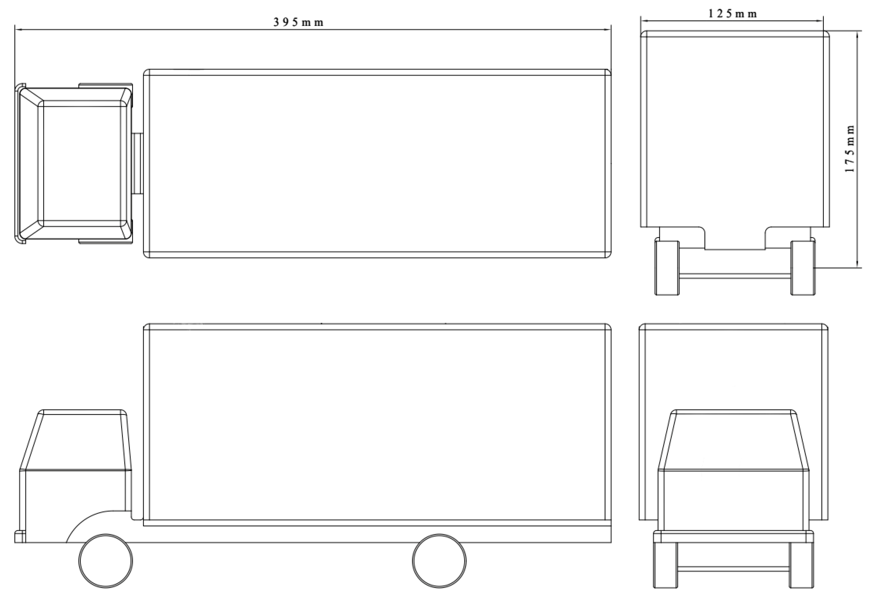
2.1. Scene Determination and Model Selection
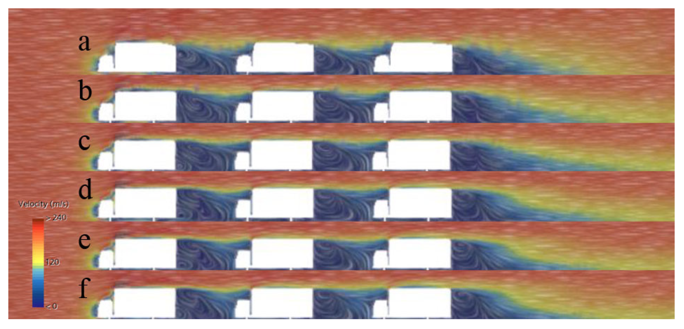
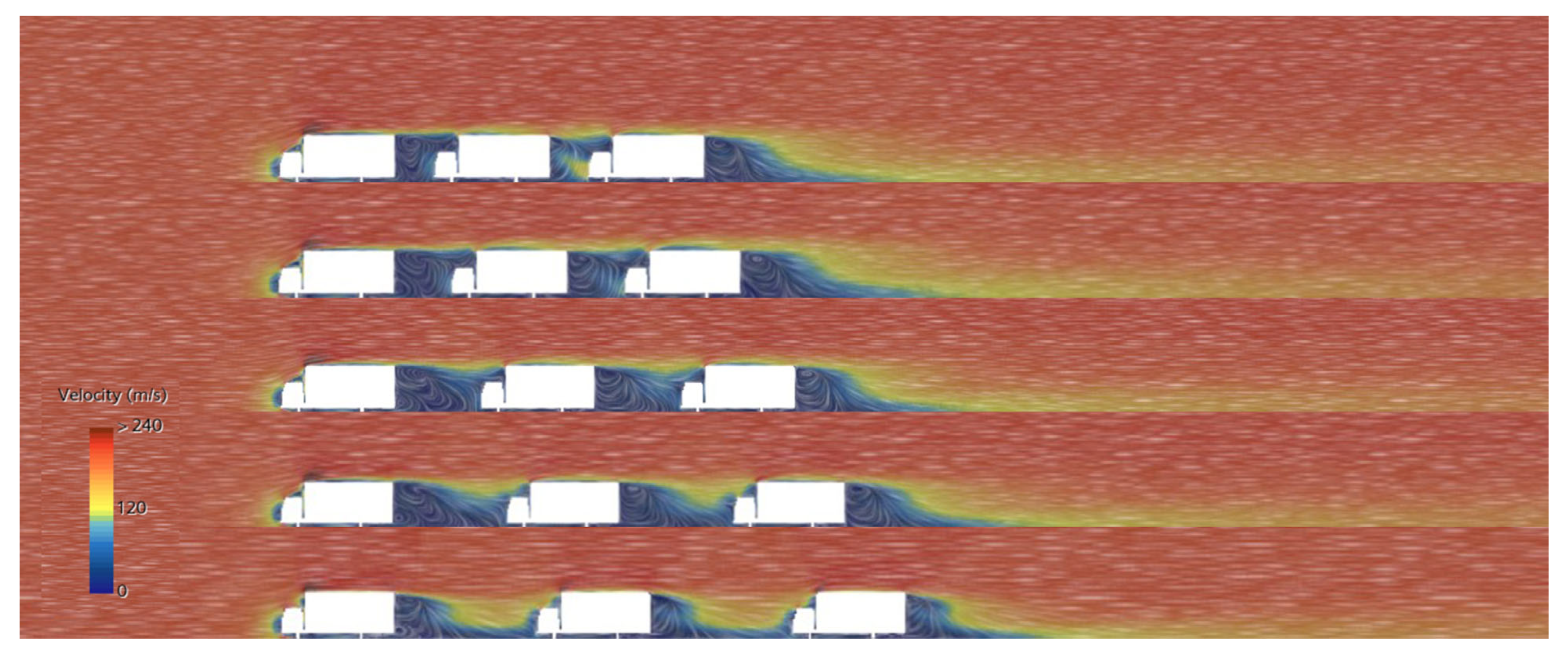
2.2. Experimental Data of Computational Fluid Dynamics
- Step 1: Identification of the study region: A cube with dimensions of 7000 mm, 1500 mm, and 1200 mm is established in the simulation. Specifically, entrance and exit boundaries, two side boundaries, top and bottom boundaries are generated. To determine the study region, the Boolean subtraction function in STAR-CCM+ 2302 can be used to create the surrounding area where the vehicle travels, and prepare the final region for mesh division.
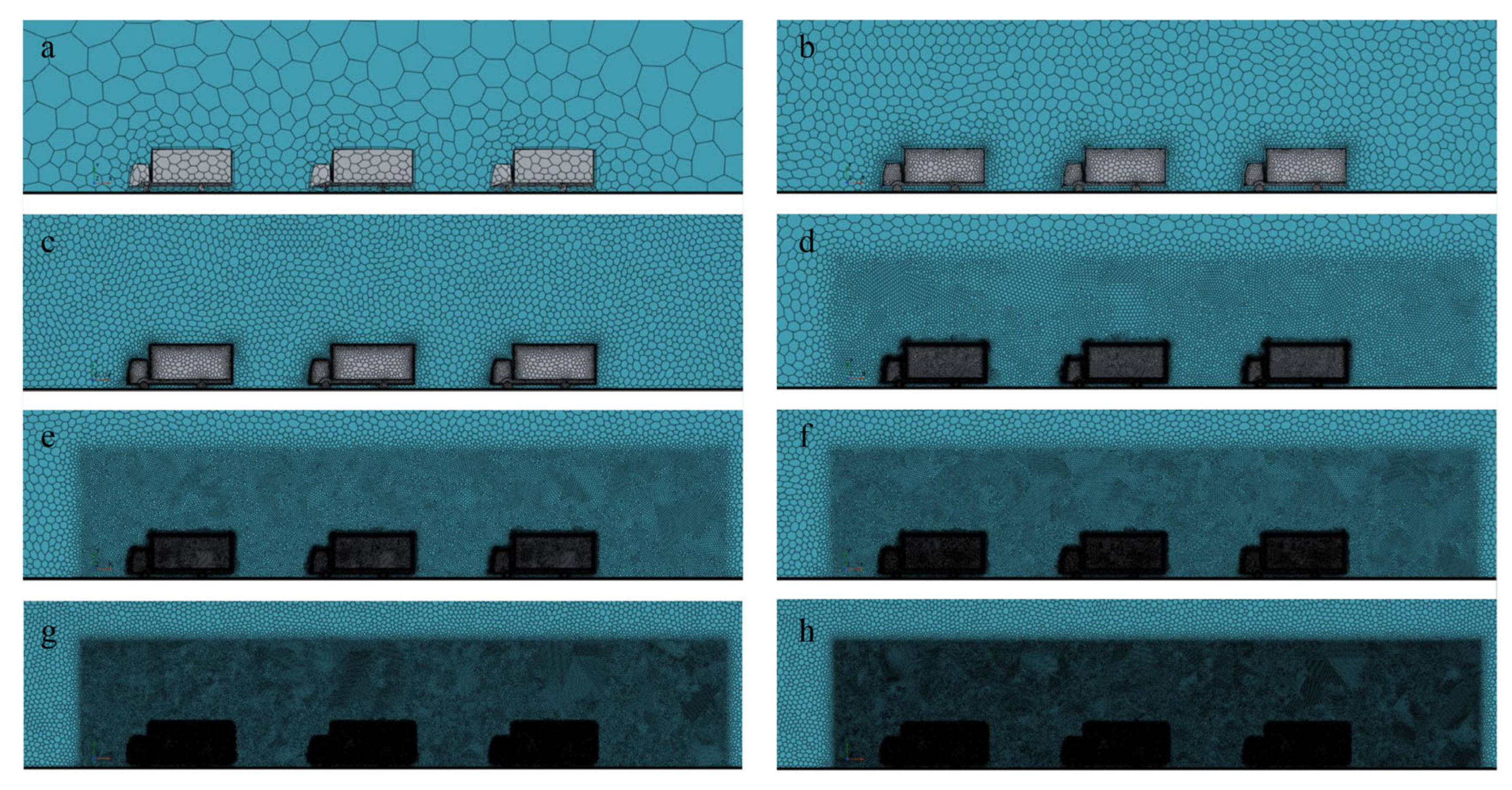
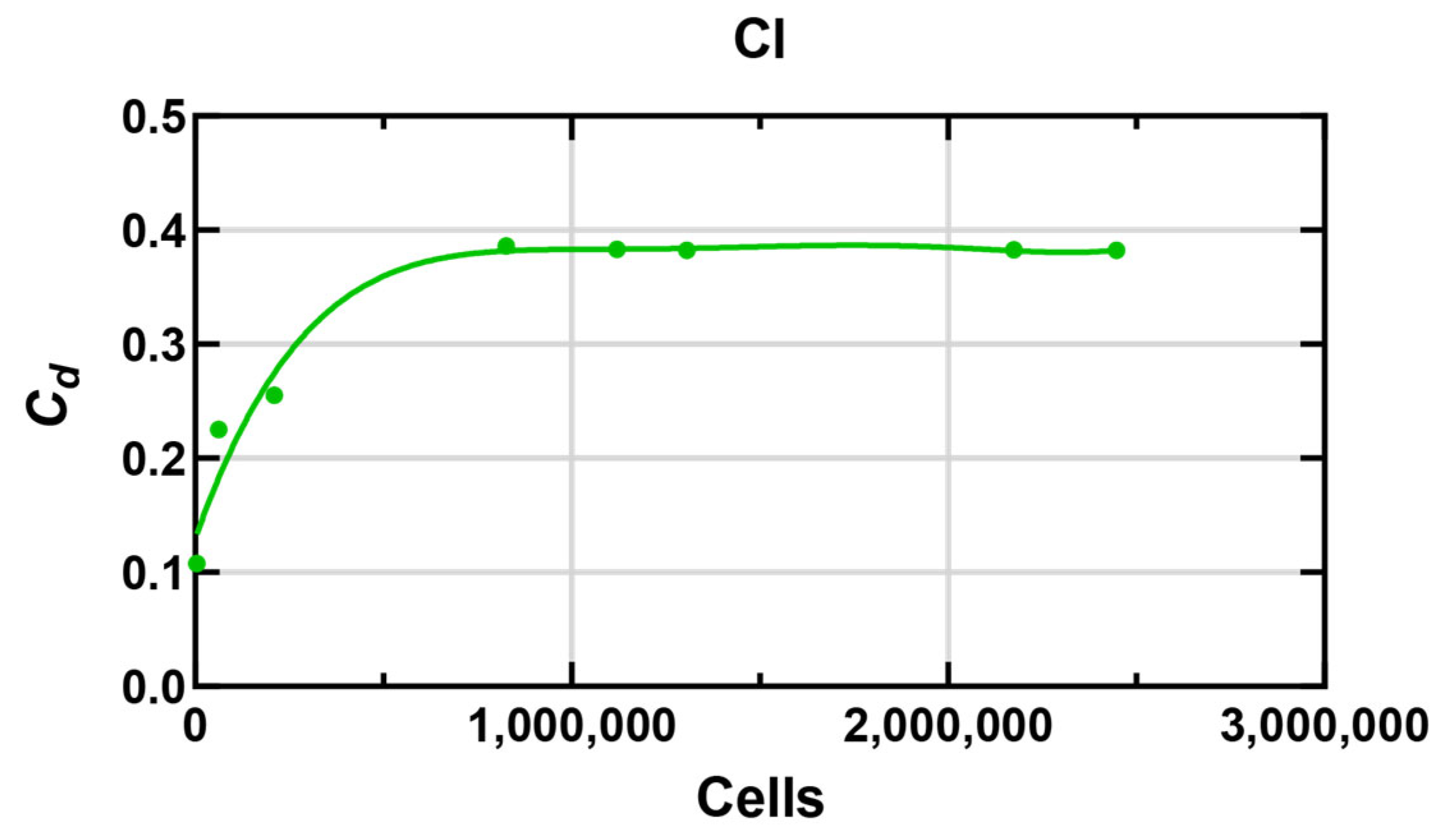
- Step 2: Meshing: After verifying the mesh independence analysis, the mesh size was determined. Generate a basic mesh through the “automatic mesh” function. The base size of the mesh is 0.04, the mesh growth rate is set to 1.3, the number of prism layers is 4, the prism layer extension is 1.2, and the total thickness of the prism layers (absolute value) is 0.008 m. Then use custom controls for fine adjustment to refine the grid on the surface of the vehicle, while increasing the grid refinement in the vicinity of the vehicle as shown in Figure 2e. The final number of cells is 994,915.
- Step 3: In the study region, the inlet and outlet boundaries of the fluid direction are defined as velocity inlet and pressure outlet. The top and bottom are defined as the wall surface. The side is defined as a symmetrical face. The speed of velocity inlet is set to 200 m/s. The pressure outlet is set to 0. Dynamic viscosity and fluid density . Thus, the computational fluid dynamics Reynolds number .
3. Establishment of the Online Prediction Model for Aerodynamic Performance of Platooning Vehicles
3.1. Stacking Ensemble Learning Principle
3.2. Base Learner Model Construction
- RF algorithm.
- A subset T(t) is obtained by sampling back from T;
- Select randomly features to construct candidate feature set F(t), where ρ is the sampling rate;
- Recursively partition nodes until stopping conditions are met, and the splitting criterion is minimized using the Gini exponent:
- 2.
- XGBoost algorithm.
3.3. Meta-Learner Model Construction
- Step 1: RF algorithm is adopted as a primary learner to perform a 5-fold cross-validation method with K = 5. The original training set is divided equally into five mutually exclusive subsets, marked as {Train 1, Train 2, …, Train5}.
- Step 2: Perform hierarchical cross-training to cross-validate prediction results. Select {Train 1–Train 4} as training subset and Train 5 as validation subset in the first iteration, and output validation prediction RF-Predic5. Select {Train 1–Train 3, Train 5} as training subset and Train 4 as validation subset in the second iteration, and generate RF-Predic 4. Repeat the above process until five rounds of validation are completed, and finally construct prediction matrix [RF-Predic 1]–[RF-Predic5].
- Step 3: Integrating the five-dimensional prediction results generated in step 2 to form a meta-learning layer training feature matrix X_meta_train ∈ ℝ^{N × 5} (N is the total sample size).
- Step 4: Test set feature extraction. Five groups of independent predictions are conducted on the original test set based on the reconstructed RF model of the complete training set. Calculate the predicted mean value AVGRF-Predict ∈ ℝ^{M × 1} (M is the number of test samples) of the break as the core input of the meta-learning layer test feature X_meta_test.
- Step 5: XGBoost is introduced as the second base learner, and the cross-validation process of steps 1–4 is repeated to obtain the prediction matrix [XGB-Predic1]–[XGB-Predic5] and mean of AGGXGB-Predict. Then concatenate X_meta_train and X_meta_test.
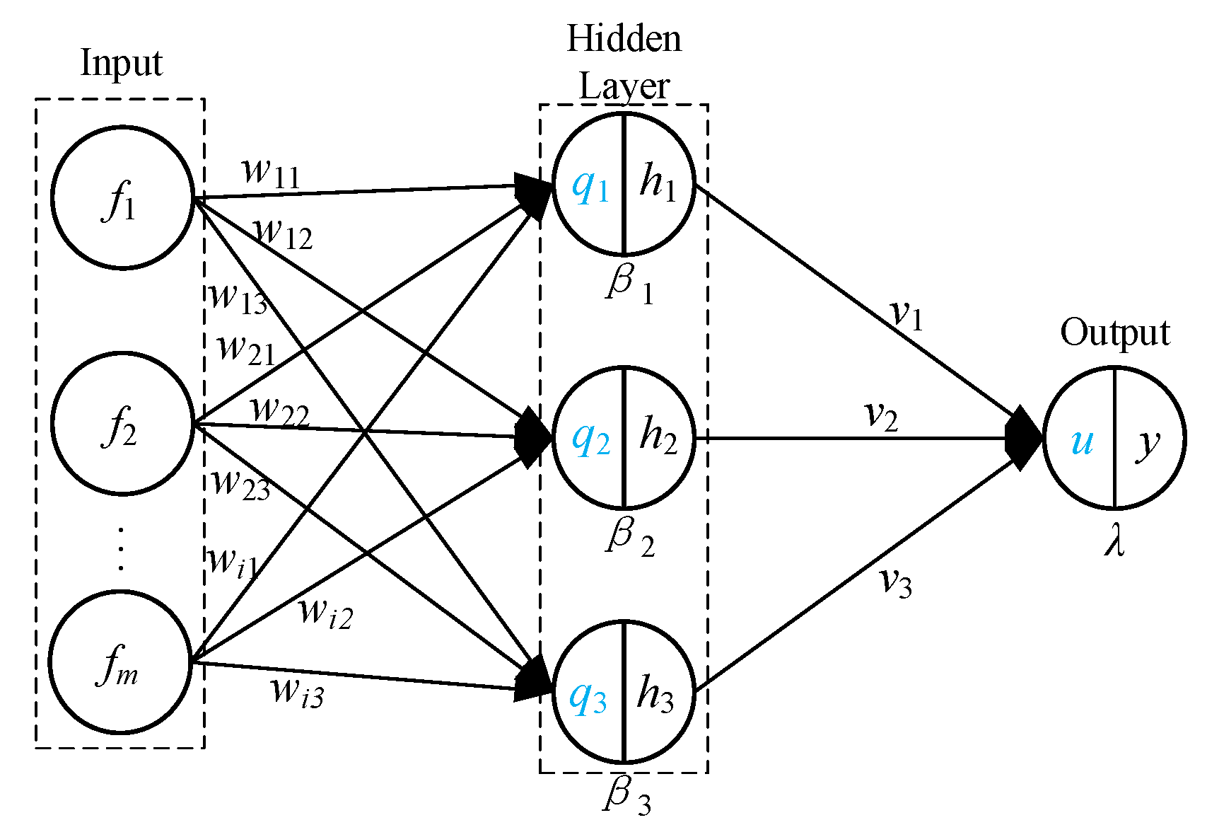
- Step 6: Construct a BP neural network with backpropagation architecture as the meta-learner model. The model receives the compound features of X_meta_train at the input layer. At the hidden layer, the model implements nonlinear mapping using the BP neural network. Through backpropagation, the model optimizes the weights and finally generates the final aerodynamic performance prediction values at the output layer, and completes model verification by utilizing X_meta_test.
3.4. Model Building and Training
3.5. Results Analysis and Application
4. Development and Application of Digital Twin System
4.1. System Development and Operating Environment
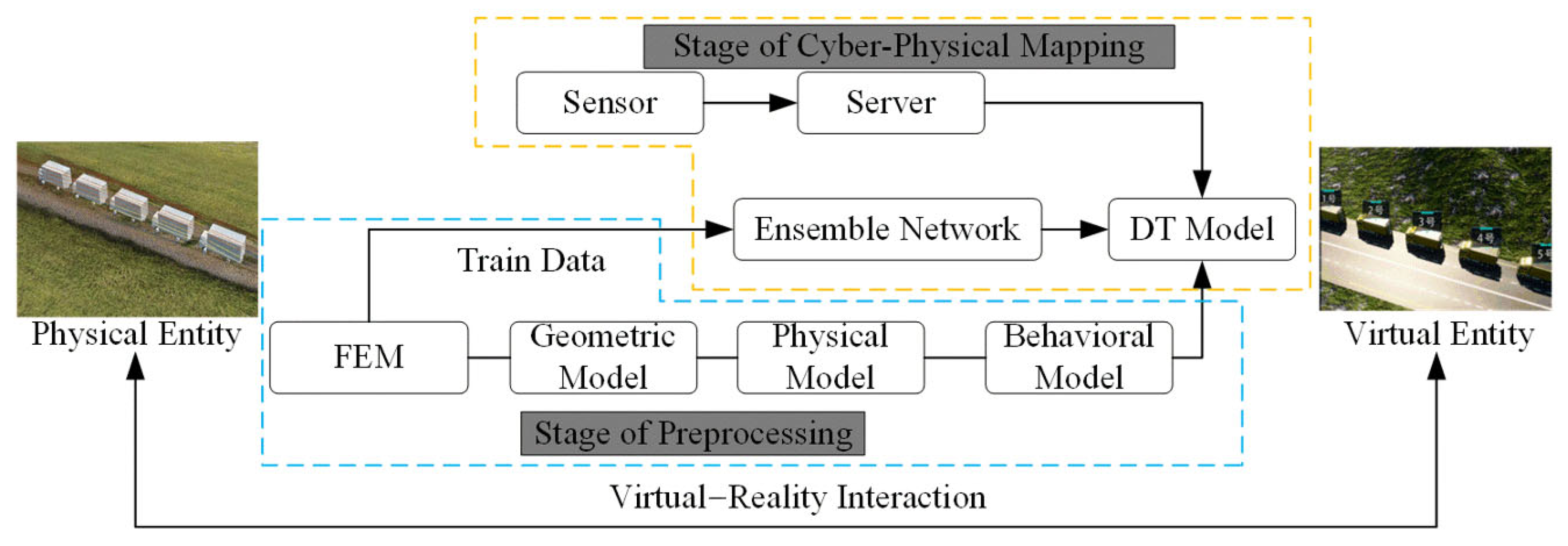
4.2. Technical Route
4.3. Introduction to System Functions
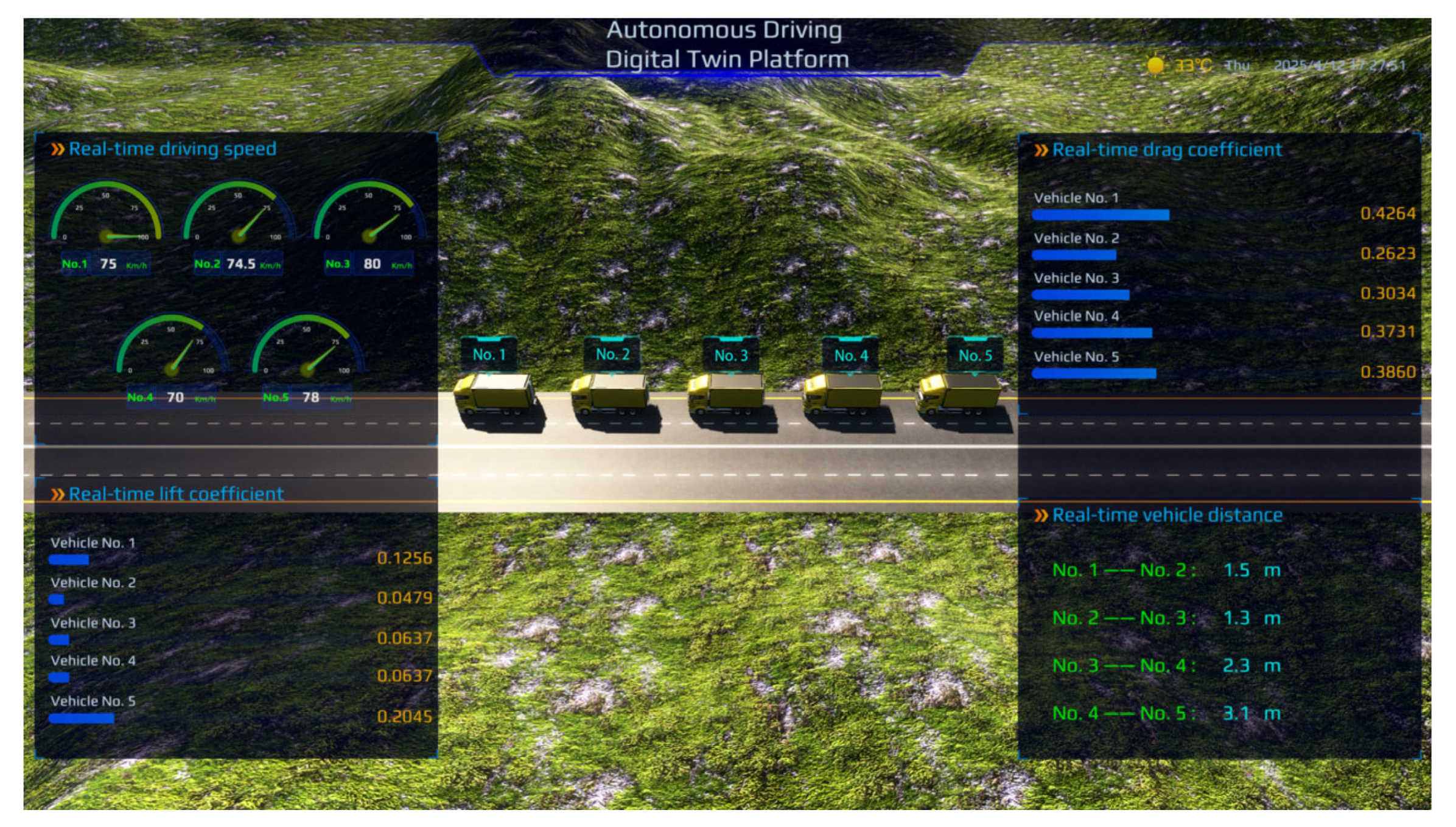
- Operation process visualization: The visualization of the lorries’ running process is the basis of the digital twin platform. With the help of the lorries’ movement model, the module displays the current running state of the lorries on the display in real time, and displays the speed and distance of the lorries’ running process on the screen in the form of lines, as shown in Figure 13a–c.
- Aerodynamic performance online monitoring: The aerodynamic performance online monitoring module is the core module of the platform. With the help of the aerodynamic performance online prediction model constructed above, the aerodynamic performance of the lorries is predicted in real time by collecting parameters such as vehicle distance and vehicle speed during the driving process, and the real-time information such as prediction data and statistical data is displayed on the display. Thus, users can fully grasp the aerodynamic performance during the operation of the lorries and improve the operation efficiency. Specifically, it includes drag coefficient and lift coefficient, as shown in Figure 13d,e.
4.4. Analysis of System Operation Results
5. Conclusions
Author Contributions
Funding
Data Availability Statement
Conflicts of Interest
References
- Xia, Y.; Jiang, L.H.; Wang, L.; Chen, X.; Ye, J.J.; Hou, T.Y.; Wang, L.Q.; Zhang, Y.B.; Li, M.Y.; Li, Z.; et al. Rapid assessments of light-duty gasoline vehicle emissions using on-road remote sensing and machine learning. Sci. Total Environ. 2022, 815, 152771. [Google Scholar] [CrossRef] [PubMed]
- Chen, X.; Jiang, L.H.; Xia, Y.; Wang, L.; Ye, J.J.; Hou, T.Y.; Zhang, Y.B.; Li, M.Y.; Li, Z.; Song, Z.; et al. Quantifying on-road vehicle emissions during traffic congestion using updated emission factors of light-duty gasoline vehicles and real-world traffic monitoring big data. Sci. Total Environ. 2022, 847, 157581. [Google Scholar] [CrossRef] [PubMed]
- Teixeira, A.C.R.; Machado, P.G.; Collaço, F.M.D.; Mouette, D. Alternative fuel technologies emissions for road heavy-duty trucks: A review. Environ. Sci. Pollut. Res. 2021, 28, 20954–20969. [Google Scholar] [CrossRef]
- Tsugawa, S.; Jeschke, S.; Shladover, S.E. A Review of Truck Platooning Projects for Energy Savings. IEEE Trans. Intell. Veh. 2016, 1, 68–77. [Google Scholar] [CrossRef]
- Turri, V.; Besselink, B.; Johansson, K.H. Cooperative Look-Ahead Control for Fuel-Efficient and Safe Heavy-Duty Vehicle Platooning. IEEE Trans. Control Syst. Technol. 2017, 25, 12–28. [Google Scholar] [CrossRef]
- Blocken, B.; Toparlar, Y.; Andrianne, T. Aerodynamic benefit for a cyclist by a following motorcycle. J. Wind Eng. Ind. Aerodyn. 2016, 155, 1–10. [Google Scholar] [CrossRef]
- Weimerskirch, H.; Martin, J.; Clerquin, Y.; Alexandre, P.; Jiraskova, S. Energy saving in flight formation—Pelicans flying in a ‘V’ can glide for extended periods using the other birds’ air streams. Nature 2001, 413, 697–698. [Google Scholar] [CrossRef]
- Katz, J. Aerodynamics of race cars. Annu. Rev. Fluid Mech. 2006, 38, 27–63. [Google Scholar] [CrossRef]
- Khan, S.; Niaz, A.; Yinke, D.; Shoukat, M.U.; Nawaz, S.A. Deep reinforcement learning and robust SLAM based robotic control algorithm for self-driving path optimization. Front. Neurorobot. 2025, 18, 1428358. [Google Scholar] [CrossRef]
- Massar, M.; Reza, I.; Rahman, S.M.; Abdullah, S.M.H.; Jamal, A.; Al-Ismail, F.S. Impacts of Autonomous Vehicles on Greenhouse Gas Emissions-Positive or Negative? Int. J. Environ. Res. Public Health 2021, 18, 5567. [Google Scholar] [CrossRef]
- Grieves, M. Product lifecycle management: The new paradigm for enterprises. Int. J. Prod. Dev. 2005, 2, 71–84. [Google Scholar] [CrossRef]
- Liu, X.; Jiang, D.; Tao, B.; Xiang, F.; Jiang, G.; Sun, Y.; Kong, J.; Li, G. A systematic review of digital twin about physical entities, virtual models, twin data, and applications. Adv. Eng. Inf. 2023, 55, 101876. [Google Scholar] [CrossRef]
- Jones, D.; Snider, C.; Nassehi, A.; Yon, J.; Hicks, B. Characterising the Digital Twin: A systematic literature review. CIRP J. Manuf. Sci. Technol. 2020, 29, 36–52. [Google Scholar] [CrossRef]
- Tao, F.; Xiao, B.; Qi, Q.; Cheng, J.; Ji, P. Digital twin modeling. J. Manuf. Syst. 2022, 64, 372–389. [Google Scholar] [CrossRef]
- Verna, E.; Genta, G.; Galetto, M.; Franceschini, F. Defect prediction for assembled products: A novel model based on the structural complexity paradigm. Int. J. Adv. Manuf. Technol. 2022, 120, 3405–3426. [Google Scholar] [CrossRef]
- Han, C.; Zhou, G.; Zhang, C.; Yu, Y.; Ma, D. A novel framework for online decision-making and feedback optimization of complex products process parameter based on edge-cloud collaboration. Digit. Twin 2022, 2, 13. [Google Scholar] [CrossRef]
- Veldhuizen, R.; Van Raemdonck, G.M.R.; van der Krieke, J.P. Fuel economy improvement by means of two European tractor semi-trailer combinations in a platooning formation. J. Wind Eng. Ind. Aerodyn. 2019, 188, 217–234. [Google Scholar] [CrossRef]
- Maiti, S.; Winter, S.; Kulik, L. A conceptualization of vehicle platoons and platoon operations. Transp. Res. Part C Emerg. Technol. 2017, 80, 1–19. [Google Scholar] [CrossRef]
- Neto, C.; Simoes, A.; Cunha, L.; Pedro Duarte, S.; Lobo, A. Qualitative data collection to identify truck drivers’ attitudes toward a transition to platooning systems. Accid. Anal. Prev. 2024, 195, 107405. [Google Scholar] [CrossRef]
- He, M.; Huo, S.; Hemida, H.; Bourriez, F.; Robertson, F.H.; Soper, D.; Sterling, M.; Baker, C. Detached eddy simulation of a closely running lorry platoon. J. Wind Eng. Ind. Aerodyn. 2019, 193, 103956. [Google Scholar] [CrossRef]
- Song, J.; Wang, W.T.; Li, L.; Liang, L.R. Injection molding part size prediction method based on stacking ensemble learning. J. South China Univ. Technol. (Nat. Sci. Ed.) 2022, 50, 19–26. [Google Scholar] [CrossRef]
- Janitza, S.; Tutz, G.; Boulesteix, A.-L. Random forest for ordinal responses: Prediction and variable selection. Comput. Stat. Data Anal. 2016, 96, 57–73. [Google Scholar] [CrossRef]
- Wu, J.; Fang, L.C.; Liu, X.T.; Chen, J.J.; Liu, X.J.; Lü, B. State of health estimation of lithium-ion battery based on feature optimization and random forest algorithm. J. Mech. Eng. 2024, 60, 335–343. [Google Scholar]
- Jiang, S.F.; Wu, T.J.; Peng, X.; Li, J.Q.; Li, Z.; Sun, T. Data Driven Fault Diagnosis Method Based on XGBoost Feature Extraction. Chin. J. Mech. Eng. 2020, 31, 1232–1239. [Google Scholar] [CrossRef]
- Zhang, Y.; Chen, B.; Pan, G.; Zhao, Y. A novel hybrid model based on VMD-WT and PCA-BP-RBF neural network for short-term wind speed forecasting. Energy Convers. Manag. 2019, 195, 180–197. [Google Scholar] [CrossRef]


| Group | Number of Cells | Base Size | Prism Layer Numbers | Lorries Surface Control | Refinement Regions Control | Drag Coefficient |
|---|---|---|---|---|---|---|
| a | 4321 | 0.3 | 1 | None | None | 0.107697 |
| b | 62,689 | 0.05 | 1 | None | None | 0.225347 |
| c | 210,589 | 0.03 | 4 | None | None | 0.255347 |
| d | 826,539 | 0.05 | 4 | 10% relative to the base size | 25% relative to the base size | 0.386238 |
| e | 1,119,995 | 0.04 | 4 | 10% relative to the base size | 25% relative to the base size | 0.383351 |
| f | 1,306,744 | 0.035 | 4 | 10% relative to the base size | 25% relative to the base size | 0.382107 |
| g | 2,174,597 | 0.02 | 4 | 10% relative to the base size | 25% relative to the base size | 0.382519 |
| h | 2,447,670 | 0.02 | 4 | 10% relative to the base size | 20% relative to the base size | 0.382230 |
| Lorry Spacing | Single Lorry | 1.27L (500 mm) | 1.01L (400 mm) | 0.76L (300 mm) | 0.51L (200 mm) | 0.25L (100 mm) |
|---|---|---|---|---|---|---|
| 0.66 | 0.4125 | 0.3937 | 0.3830 | 0.3496 | 0.3097 | |
| Reduction | 0% | 37.50% | 40.35% | 41.97% | 47.03% | 53.08% |
| RF Model | XGBoost Model (Gradient-Boosted Tree) | ||
|---|---|---|---|
| Number of decision trees | 200 | Learning Rate and regularization | 0.025 |
| Maximum depth | 10 | Maximum depth | 10 |
| Minimum number of separated samples | 100 | Complexity penalty term | 0.1 |
| Maximum characteristic number of a single node | 5 | Total number of lifting trees | 200 |
| Optimizer | Optimizer Type | Adam |
|---|---|---|
| Default Learning Rate | 10−3 | |
| Regularization Mechanism | Regularization Type | Dropout |
| Rate | 0.2 | |
| Training Configuration | batch_siz | 64 |
| epoch | 500 |
| Test | Fr | Fr1 | Fr2 | Fr3 | Test | Fr1 | Fr2 | Fr3 |
|---|---|---|---|---|---|---|---|---|
| T1 | STBP_Pred | 0.449 | 0.279 | 0.245 | T5 | 0.459 | 0.256 | 0.331 |
| BP_Pred | 0.512 | 0.254 | 0.231 | 0.206 | 0.198 | 0.271 | ||
| True | 0.448 | 0.273 | 0.248 | 0.451 | 0.252 | 0.333 | ||
| Acc_STBP | 0.997 | 0.977 | 0.987 | 0.982 | 0.984 | 0.994 | ||
| Acc_BP | 0.856 | 0.932 | 0.931 | 0.457 | 0.786 | 0.814 | ||
| T2 | STBP_Pred | 0.470 | 0.227 | 0.304 | T6 | 0.510 | 0.338 | 0.367 |
| BP_Pred | 0.442 | 0.207 | 0.386 | 0.382 | 0.408 | 0.455 | ||
| True | 0.476 | 0.231 | 0.298 | 0.515 | 0.341 | 0.371 | ||
| Acc_STBP | 0.987 | 0.983 | 0.980 | 0.990 | 0.991 | 0.989 | ||
| Acc_BP | 0.929 | 0.896 | 0.705 | 0.742 | 0.804 | 0.774 | ||
| T3 | STBP_Pred | 0.482 | 0.292 | 0.331 | T7 | 0.499 | 0.335 | 0.370 |
| BP_Pred | 0.301 | 0.228 | 0.281 | 0.341 | 0.442 | 0.298 | ||
| True | 0.489 | 0.287 | 0.337 | 0.491 | 0.338 | 0.362 | ||
| Acc_STBP | 0.992 | 0.983 | 0.991 | 0.984 | 0.991 | 0.978 | ||
| Acc_BP | 0.581 | 0.703 | 0.839 | 0.695 | 0.692 | 0.823 | ||
| T4 | STBP_Pred | 0.347 | 0.279 | 0.331 | T8 | 0.472 | 0.243 | 0.320 |
| BP_Pred | 0.203 | 0.215 | 0.368 | 0.304 | 0.348 | 0.238 | ||
| True | 0.354 | 0.285 | 0.339 | 0.476 | 0.248 | 0.316 | ||
| Acc_STBP | 0.980 | 0.979 | 0.976 | 0.992 | 0.980 | 0.987 | ||
| Acc_BP | 0.573 | 0.754 | 0.914 | 0.639 | 0.597 | 0.753 |
| Hardware Environment | CPU: Intel(R) Xeno(R) Gold 5218 CPU @ 2.30 Ghz 2.29 Ghz; Running Memory: 256 GB; Hard Disk: 4 T; GPU: NVIDIA Quadro RTX4000 | |
|---|---|---|
| Software Environment | Operating System | Windows 10 |
| Development Languages and Frameworks | C#, Python 3.10, scikit-learn, Net Framework 4.7.2 | |
| Database | MySQL 8.0.23 | |
| Development Platform | Microsoft visual studio 2020, Pycharm 2021.1.3, Unity 2020.3.40 | |
Disclaimer/Publisher’s Note: The statements, opinions and data contained in all publications are solely those of the individual author(s) and contributor(s) and not of MDPI and/or the editor(s). MDPI and/or the editor(s) disclaim responsibility for any injury to people or property resulting from any ideas, methods, instructions or products referred to in the content. |
© 2025 by the authors. Licensee MDPI, Basel, Switzerland. This article is an open access article distributed under the terms and conditions of the Creative Commons Attribution (CC BY) license (https://creativecommons.org/licenses/by/4.0/).
Share and Cite
Wang, Z.; Guo, X.; Yang, N.; Su, L.; Chen, L.; Zhang, Z.; Zhu, C. Research on Data Prediction Model for Aerodynamic Drag Reduction Effect in Platooning Vehicles. Processes 2025, 13, 2056. https://doi.org/10.3390/pr13072056
Wang Z, Guo X, Yang N, Su L, Chen L, Zhang Z, Zhu C. Research on Data Prediction Model for Aerodynamic Drag Reduction Effect in Platooning Vehicles. Processes. 2025; 13(7):2056. https://doi.org/10.3390/pr13072056
Chicago/Turabian StyleWang, Zhexin, Xuepeng Guo, Ning Yang, Lingjun Su, Lu’an Chen, Zhao Zhang, and Chengyu Zhu. 2025. "Research on Data Prediction Model for Aerodynamic Drag Reduction Effect in Platooning Vehicles" Processes 13, no. 7: 2056. https://doi.org/10.3390/pr13072056
APA StyleWang, Z., Guo, X., Yang, N., Su, L., Chen, L., Zhang, Z., & Zhu, C. (2025). Research on Data Prediction Model for Aerodynamic Drag Reduction Effect in Platooning Vehicles. Processes, 13(7), 2056. https://doi.org/10.3390/pr13072056