Abstract
To address the challenges posed by the volatility and uncertainty of wind power generation, this study presents a hybrid model combining complete ensemble empirical mode decomposition with adaptive noise (CEEMDAN), variational mode decomposition (VMD), convolutional neural network (CNN), and bidirectional long short-term memory (BiLSTM) for wind power forecasting. The model first employs CEEMDAN to decompose the original wind power sequence into multiple scales, obtaining several intrinsic mode functions (IMFs). These IMFs are then classified using sample entropy and k-means clustering, with high-frequency IMFs further decomposed using VMD. Next, the decomposed signals are processed by a CNN to extract local spatiotemporal features, followed by a BiLSTM network that captures bidirectional temporal dependencies. Experimental results demonstrate the superiority of the proposed model over ARIMA, LSTM, CEEMDAN-LSTM, and VMD-CNN-LSTM models. The proposed model achieves a mean squared error (MSE) of 67.145, a root mean squared error (RMSE) of 8.192, a mean absolute error (MAE) of 6.020, and a coefficient of determination (R2) of 0.9840, indicating significant improvements in forecasting accuracy and reliability. This study offers a new solution for enhancing wind power forecasting precision, which is crucial for efficient grid operation and energy management.
1. Introduction
In the global energy structure’s accelerated transition toward low-carbon systems, wind power, with its clean and renewable advantages, has become a key part of power systems [1,2,3]. Statistics from the International Renewable Energy Agency (IRENA) show that China maintained its leading position in global wind power installed capacity as of 2021 [4]. However, wind power generation, influenced by complex meteorological conditions and equipment operation status, exhibits significant volatility and uncertainty [5]. This poses severe challenges to grid scheduling, electricity market trading, and equipment maintenance, making high-precision power forecasting technology essential [6].
Currently, wind power forecasting methods are mainly categorized into physical models, statistical models, and data-driven approaches. Physical models, based on aerodynamic principles, have explicit physical meanings but are highly dependent on meteorological and equipment parameters and struggle to capture nonlinear characteristics [7]. Statistical models like ARIMA and SVM predict by fitting historical data, but lack adaptability to non-stationary and nonlinear data. In recent years, deep learning has emerged as a new tool for wind power forecasting [8].
Early wind power forecasting studies focused on physical modeling. For instance, a study in [9] built a unit model based on aerodynamics and predicted power using meteorological data. While the physical significance was clear, calibration difficulties in complex terrains and variable weather limited forecasting accuracy. On the statistical modeling front, the authors of [10] used ARMA and other time-series methods, relying on statistical patterns for modeling. This approach was computationally simple but insufficient for non-stationary and nonlinear data. With AI development, machine learning methods gained traction. SVM, through kernel functions, enabled nonlinear fitting. As shown in [11], SVM was applied to wind power forecasting with some success, but its performance heavily relied on parameter tuning and had computational efficiency limits. Deep learning techniques introduced a breakthrough, with LSTM and its variants capturing long-term dependencies in time-series data through gating mechanisms. As demonstrated in [12], LSTM significantly improved forecasting accuracy but had weak spatial feature extraction capabilities. CNN excelled at extracting local spatiotemporal features but fell short in modeling long-term temporal dependencies [13]. To leverage the strengths of different methods, hybrid models became a research hotspot. For example, Ref. [14] proposed a VMD-LSTM model that first used variational mode decomposition to extract multi-scale features and then predicted with LSTM, effectively enhancing accuracy. Another study in [15] combined CNN-LSTM to handle spatial and temporal features separately, further refining forecasting outcomes. In China, initial research focused on improving traditional models. For instance, Ref. [16] enhanced time-series models’ adaptability to non-stationary data through seasonal adjustments and differencing. In deep learning, [17] introduced attention mechanisms to strengthen LSTM’s focus on key temporal sequences, while [18] improved model robustness through data cleaning.
However, existing methods have limitations. Statistical models like ARIMA are computationally simple but lack adaptability to non-stationary and nonlinear data. Machine learning methods offer strong nonlinear fitting but depend on parameter tuning and have computational efficiency limits. LSTM captures long-term temporal dependencies but weakly extracts spatial features, while CNN effectively extracts local spatiotemporal features but falls short in modeling long-term temporal dependencies. These limitations highlight the need for new solutions in wind power forecasting.
To address these issues, this study proposes a deep forecasting model integrating multi-source information and adaptive decomposition. The model constructs a multi-source data fusion framework, enhances signal decomposition with CEEMDAN and VMD, and designs a CNN-BiLSTM network with dual attention mechanisms to capture key spatiotemporal and equipment status features. Experimental results show that the proposed model achieves superior forecasting accuracy with an MSE of 67.145, RMSE of 8.192, MAE of 6.020, and R2 of 0.9840, offering a new technical solution for wind power forecasting.
The structure of this paper is as follows:
Section 2 introduces the theoretical foundations of the proposed model, including signal decomposition algorithms (CEEMDAN and VMD), sample entropy, k-means clustering, and deep learning frameworks (CNN and BiLSTM).
Section 3 details the construction of the CEEMDAN-VMD-CNN-BiLSTM model, covering data preprocessing, model architecture design, and parameter optimization strategies.
Section 4 presents experimental results, including signal decomposition analysis, performance comparisons with other models, and discussion of forecasting accuracy metrics (MSE, RMSE, MAE, and R2).
Section 5 summarizes the research conclusions and outlines future work directions for model optimization and computational efficiency improvement.
The list of acronyms is shown in Table 1.

Table 1.
List of abbreviations.
2. Theoretical Basis
2.1. CEEMDAN
We use the CEEMDAN algorithm to perform multi-scale decomposition on the original wind power generation series, generating IMF components at different frequencies. CEEMDAN solves the mode-mixing problem of traditional EMD methods in processing non-stationary signals [19] and is particularly suitable for multi-scale analysis of complex fluctuating signals such as wind power [20]. The algorithm decomposes the original signal into intrinsic mode function (IMF) components of different frequencies through multi-scale decomposition, in which high-frequency components reflect short-term rapid fluctuations and low-frequency components represent long-term trends, thus achieving multi-scale separation of complex signals [21]. In this paper, the preprocessed forecast dataset is first decomposed using CEEMDAN. The process is as follows:
- Adding white noise:
- First-order intrinsic mode component C1(k):
- IMF of the first iteration:
- Residual r1(t):
- Iterative decomposition: The above steps are repeated to successively extract C2(t), C3(t), …, until the residual rm(t) becomes a monotonic signal. Finally, the original signal y(t) is decomposed into m IMF components and one residual:
The process of CEEMDAN calculation is shown in Figure 1. CEEMDAN performs multi-scale decomposition on the original signal by adding Gaussian white noise and multiple ensemble averaging. It iteratively extracts intrinsic mode function (IMF) components of different frequencies from the signal, and the residual after decomposition becomes a monotonic signal.
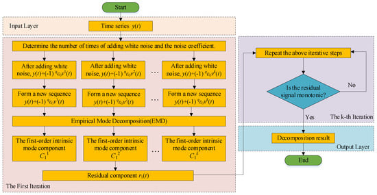
Figure 1.
Flowchart for CEEMDAN.
2.2. Sample Entropy Calculation
After CEEMDAN decomposition, the IMF components are quantified for their complexity features using sample entropy. In wind power data, high-frequency IMF components usually contain more noise and random fluctuations, resulting in higher sample entropy values, while low-frequency IMF components tend to contain more regular trend information, leading to lower sample entropy values. The steps are as follows [22]:
- Embed the time-series x into an m-dimensional space to construct embedding vectors:
- For each embedding vector Xim, calculate the Euclidean distance dij to all other embedding vectors Xim.
- Set the similarity tolerance r, typically r = 0.2std(x).
- For each Xim, calculate the proportion of embedding vectors Cim(r) that satisfy dij ≤ r.
- The sample entropy is defined as follows:
2.3. K-Means Clustering
Wind power data typically contain fluctuation components across different time scales. Therefore, IMF components with similar sample entropy values are k-means clustering into groups, which can generally be categorized into three types: high frequency, medium frequency, and low frequency. IMF components within the same group exhibit similar complexity characteristics. The k-means clustering process is shown in Figure 2. It starts by randomly selecting initial cluster centers and then assigns each IMF component to the nearest center via Euclidean distance based on sample entropy. Cluster centers are recalculated iteratively until convergence. The calculation steps are as follows [23]:
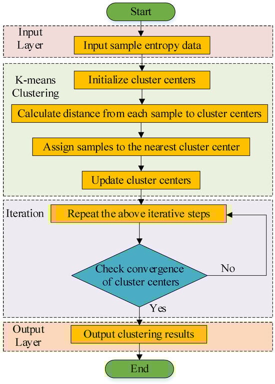
Figure 2.
Flowchart of k-means clustering.
- Randomly select k samples as the initial cluster centers C1, C2, …, Ck.
- Assign each sample xi to the nearest cluster center:
- Recalculate the center of each cluster:
- Repeat the sample assignment and cluster center update steps until the cluster centers no longer change, or the maximum number of iterations is reached.
2.4. Variational Mode Decomposition
The high-frequency IMFs obtained through clustering are decomposed using VMD to further separate the mixed modes within them. The refined decomposition results of the high-frequency IMFs are then concatenated with the medium-frequency and low-frequency IMFs.
VMD is a method that transforms the signal decomposition problem into solving the center frequency and bandwidth of each mode by constructing a variational optimization model, thus avoiding endpoint effects and mode mixing. It is suitable for multi-scale analysis of nonlinear and non-stationary signals [24,25]. As shown in Figure 3, the VMD process includes the following steps: assuming the signal is decomposed into k sub-signals (modes); constructing a variational problem with a penalty factor α and a Lagrange multiplier λ(t); and iteratively updating the modal parameters and the multiplier until the convergence criterion ε is met:
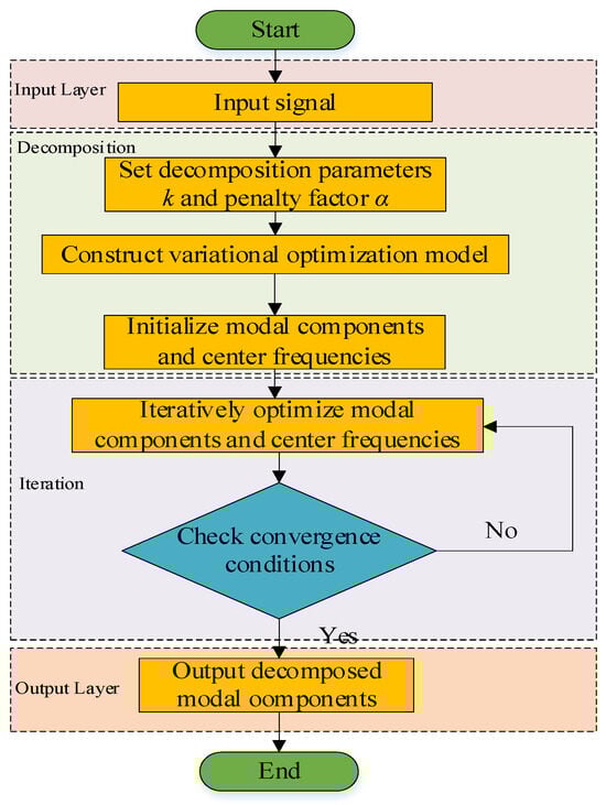
Figure 3.
VMD flowchart.
(1) Assume the signal f(t) to be processed:
In the above formula, ωk is the center frequency of the k-th mode, and δ(t) is the unit impulse function. Here, k is the number of modes obtained from the decomposition, and the input signal f(t) is decomposed into discrete sub-signals (modes) μk.
(2) Solve the variational problem:
where α is the penalty factor, λ(t) is the Lagrange multiplier, and the last term is an additional constraint. The parameters are initialized and updated according to Equations (12)–(14) until Equation (15) is satisfied.
where τ is the noise tolerance, and ε is the convergence criterion.
Spectral analysis is used to display the frequency characteristics of each decomposed modal component. The mathematical expressions are as follows:
Fast Fourier Transform (FFT): Perform FFT on each modal component uk(t):
Amplitude Spectrum: Calculate the amplitude of the FFT result:
Set the frequency range to [0, fs/2], where fs is the sampling frequency.
2.5. CNN
CNN consists of an input layer, convolutional layers, a ReLU activation layer, max-pooling layers, a flattening layer, a BiLSTM layer, a dropout layer, fully connected layers, and a regression layer. This structure enables the CNN to effectively capture the spatiotemporal correlation characteristics in wind power forecasting [26,27]. The CNN learns the nonlinear relationships between wind direction, wind speed, and power, identifying power response patterns associated with specific wind direction combinations. The spatial features extracted by the CNN serve as inputs to the BiLSTM, allowing it to integrate historical and future information through its gating mechanism. This combination enhances the accuracy of predicting the dynamic changes in wind power.
2.6. BILSTM
BiLSTM network enhances time-series forecasting by processing data in both forward and backward directions, creating a bidirectional information flow. This allows the model to learn from both past and future data simultaneously [28,29]. The forward network processes the input sequence in chronological order, capturing feature evolutions from past to present, while the backward network processes the data in reverse, uncovering hidden relationships from future to past. In wind power forecasting, BiLSTM’s bidirectional processing enables it to capture both historical power fluctuations and potential future meteorological impacts. The forward network learns the temporal patterns of historical power and meteorological data, while the backward network infers current key features from future data, improving forecasting accuracy.
Among them, and represent the forward and backward LSTM outputs, respectively. wt and vt are the output weights of each hidden layer, and LSTM(∙) denotes the LSTM calculation process. The structure of BiLSTM is shown in Figure 4. It processes data bidirectionally, with forward and backward LSTMs capturing past and future info. Inputs x1–x3 go through hidden layers (weights w1–w3, v1–v3) to output y1–y3, enhancing forecast accuracy by integrating bidirectional temporal features. w1 to w3 and v1 to v3 are the hidden layer weights of the forward and backward LSTMs, x1 to x3 are the network input values, and y1 to y3 are the network output values.
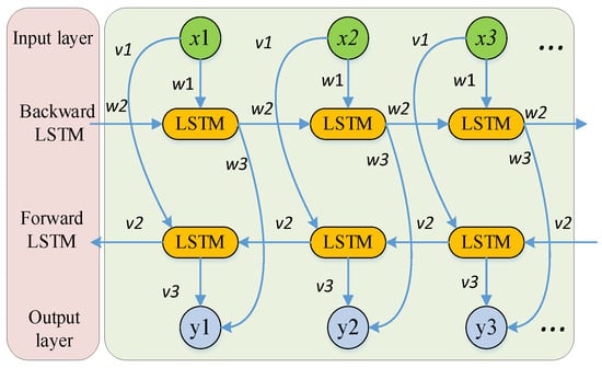
Figure 4.
BiLSTM structure.
3. Construction of CEEMDAN-VMD-CNN-BILSTM Model
3.1. Model Framework Design
3.1.1. Signal Decomposition of CEEMDAN
Initially, the CEEMDAN algorithm is employed to perform multi-scale decomposition on the original wind power sequence, generating intrinsic mode function (IMF) components at different frequencies. Sample entropy is used to measure the complexity of each IMF component, followed by k-means clustering to group similar IMFs. Based on sample entropy values, the IMFs are classified into high-frequency, medium-frequency, and low-frequency groups. High-frequency IMFs are then further decomposed using VMD for secondary decomposition.
3.1.2. CNN Spatiotemporal Feature Extraction
Convolutional layers are applied to the VMD-secondary decomposed sequences to extract local spatiotemporal features (e.g., wind speed mutations and wind direction patterns). Pooling layers compress feature dimensions and enhance robustness. After convolution, data are passed through a ReLU activation layer, followed by max pooling. The pooled feature maps are then flattened into one-dimensional vectors for input into subsequent fully connected layers.
3.1.3. BiLSTM Sequence Modeling
The flattened data enter the BiLSTM layer, which processes both forward and backward temporal information simultaneously. The hidden state of the last time step is output as a feature representation of the entire sequence. The BiLSTM output is passed through a dropout layer to prevent overfitting and improve generalization.
3.1.4. Forecasting Output
The dropout layer output is fed into a fully connected layer, which calculates and outputs predicted values based on input features. Finally, the regression layer receives the fully connected layer output and generates the final forecasting results, completing the mapping from input data to forecasting.
The workflow of the CEEMDAN-VMD-CNN-BiLSTM model is shown in Figure 5. It first decomposes the original signal via CEEMDAN, classifies IMFs by sample entropy and k-means, further decomposes high-frequency components with VMD, and then extracts spatiotemporal features via CNN and captures temporal dependencies via BiLSTM for forecasting.
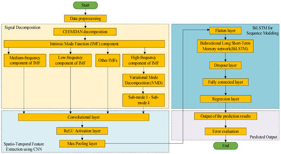
Figure 5.
The CEEMDAN-VMD-CNN-BiLSTM model structure.
3.2. Data Processing and Preparation
Generally, the original wind power forecasting data sequence contains noise, outliers, and missing values, and the dimensions and scales of different variables may also vary. Therefore, data cleaning and preprocessing are necessary [30]. For data points that deviate significantly from the normal range, thresholds are set for judgment and elimination. For example, in wind speed data, wind speeds exceeding many times the rated wind speed of the fan or negative wind speeds should be regarded as invalid data. The 3σ criterion is used to check and process data points whose deviation from the mean exceeds three times the standard deviation. Normalization ensures that data are within the same order of magnitude, facilitating subsequent model training and analysis. This study employs the min–max normalization method, with the following formula [31]:
where x represents the original wind power forecasting data sequence; xmin and xmax are the minimum and maximum values of the variable in the dataset, respectively; and xnorm is the normalized data. Through this approach, data for variables such as wind speed, wind direction, temperature, and wind power are normalized to the interval [0, 1], making the data of different variables comparable and contributing to improving the training effect and forecasting accuracy of the model.
3.3. Model Parameter Setting and Optimization
3.3.1. CEEMDAN Parameter Selection
For the CEEMDAN algorithm, the key parameters include the white noise intensity and ensemble averaging times. The selection of white noise intensity directly affects the feature enhancement effect at different scales and the mitigation of modal aliasing. If the white noise intensity is too low, it may fail to effectively enhance signal features, leaving modal aliasing unresolved. Conversely, excessive intensity may introduce noise interference and degrade decomposition accuracy [32]. Through multiple experimental comparisons, the white noise intensity is set to 0.15, and the ensemble averaging times are set to 500 in this study.
3.3.2. VMD Parameter Selection
The main parameters of the VMD algorithm are the number of modes k and the penalty factor a. The selection of k depends on the signal complexity and frequency components. An excessively small k may insufficiently decompose the signal, while an excessively large k may over-decompose it [33]. For high-frequency IMFs decomposed by CEEMDAN, spectral analysis preliminarily determines k within the range of 3–6. The penalty factor a balances signal reconstruction error and modal bandwidth. A larger a penalizes reconstruction errors more strictly, resulting in narrower modal bandwidths and higher precision but increased computational cost. A smaller a reduces bandwidth constraints and computational load but may compromise decomposition accuracy [34]. To achieve better results, the sparrow optimization algorithm (SSA) is adopted here to optimize the hyperparameters k and α, with the optimized values being k = 4 and α = 1988.
3.3.3. CNN Parameter Selection
CNN parameters include convolution kernel size, stride, number of convolutional layers, max-pooling layer size, and pooling stride [35]. A 3 × 3 convolution kernel is used with a stride of 1 to retain detailed sequence features. The ReLU activation function introduces nonlinearity to enable complex pattern learning. A 2 × 2 max-pooling layer with a stride of 2 preserves prominent features. The dropout layer randomly discards 10% of inputs to prevent overfitting. The fully connected layer outputs a single unit for regression tasks, generating forecasting values.
3.3.4. BILSTM Parameter Selection
BiLSTM parameters mainly include the number of hidden layer nodes, the learning rate, and the regularization parameter. The number of hidden layer nodes determines the model’s ability to learn temporal features. Insufficient nodes limit representational capacity, while excessive nodes increase complexity and overfitting risk [36]. In this study, the sparrow optimization algorithm (SSA) is employed to optimize the hyperparameters of BILSTM, resulting in the number of hidden layer nodes being 124, the learning rate being 0.0005, and the regularization parameter being set as 0.00001.
4. Experimental Results and Analysis
For model implementation, MATLAB 2024a was used as the development environment. The Deep Learning Toolbox was employed to construct the deep learning network. MATLAB 2024a was run on a workstation equipped with an Intel i7-12700K CPU and 32 GB of RAM.
4.1. Model Performance Evaluation Metrics
To assess the CEEMDAN-VMD-CNN-BiLSTM model’s performance, we use MSE, RMSE, MAE, and R2. These metrics are calculated as follows [37]:
where n is the number of samples, yi is the true value, is the predicted value, and is the mean of the true values. These metrics help evaluate the model’s reliability and accuracy in wind power forecasting.
4.2. Signal Decomposition
4.2.1. Data Source
To validate the effectiveness of the CEEMDAN-VMD-CNN-BiLSTM model in wind power forecasting, the dataset from the Jingxia North Wind Farm of China National Energy Group was used. The Jingxia Wind Farm is located in the Dongjingxia East Wind Area, Xiao Huangshan Dong, Qincheng Township, Yizhou District, Hami Prefecture, Xinjiang, China. The wind farm is equipped with 267 units of GW93/1500 model wind turbines (1.5 MW each) from Goldwind and 267 units of S11-1800/37 box-type transformers, with a total installed capacity of 200 MW. Jingxia Wind Farm went into operation in December 2016.
The data were collected from 1 March to 11 April 2021, including wind speeds (m/s) at 10 m, 30 m, 50 m, and 70 m, and hub height, wind directions, temperature, air pressure, humidity, and power generation, with a sampling interval of 15 min. After data cleaning and preprocessing, a total of 4000 valid data points were obtained, with 3000 in the training set and 1000 in the test set. In this study, 75% of all data were used as the training set, and 25% were used as the test set.
4.2.2. CEEMDAN Decomposition
As shown in Figure 6, the CEEMDAN algorithm decomposed the original wind power sequence into 12 intrinsic mode functions (IMFs), demonstrating its multi-scale feature extraction capability. These components captured wind power fluctuations at different frequency scales: high-frequency IMFs reflected short-term rapid changes (e.g., gusts), while low-frequency IMFs represented long-term trends (e.g., power variations due to diurnal temperature differences). By setting the white noise intensity to 0.15 and the ensemble averaging times to 500, mode mixing was effectively suppressed, ensuring the stability of decomposition results.
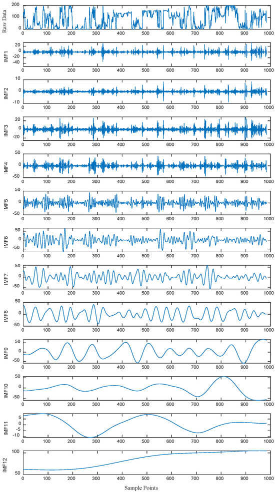
Figure 6.
CEEMDAN decomposition of wind power data.
4.2.3. Sample Entropy Calculation and K-Means Clustering
The sample entropy of each IMF was calculated to quantify sequence complexity, and k-means clustering was used to classify IMFs into high-frequency, medium-frequency, and low-frequency groups (Figure 7). Higher sample entropy values indicated higher sequence complexity, suggesting more high-frequency noise or detailed information. The clustering results showed that the high-frequency group (IMF1-IMF4) had sample entropy values > 1.2, the medium-frequency group (IMF5-IMF8) had values of 0.8–1.2, and the low-frequency group (IMF9-IMF12) had values of <0.8. This classification provided a basis for differentiated processing: high-frequency components were further decomposed by VMD to extract fine features, while medium-low frequency components were directly used for subsequent modeling.
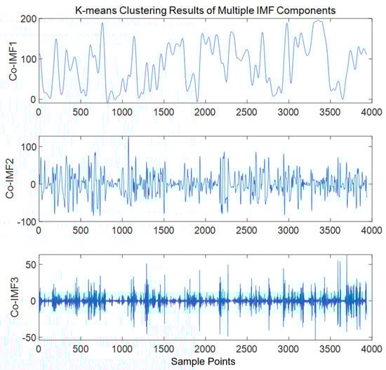
Figure 7.
K-means clustering of IMF components.
4.2.4. VMD Secondary Decomposition
For high-frequency IMF components, VMD was applied for secondary decomposition to improve feature resolution. Through spectral analysis, the decomposition mode number k = 4 and penalty factor α = 2000 were determined, further decomposing each high-frequency IMF into four sub-modes (Figure 8). The results showed that the sub-modes after secondary decomposition had more homogeneous frequency characteristics and smoother trends, effectively separating noise from real fluctuations in the original high-frequency components. This provided cleaner inputs for CNN to extract local spatiotemporal features.
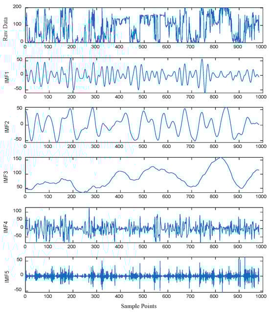
Figure 8.
VMD secondary decomposition.
4.2.5. Spectral Analysis
The spectral analysis of the sub-mode components after secondary decomposition via variational mode decomposition (VMD) was conducted using Fast Fourier Transform (FFT), and the results are illustrated in Figure 9. The analysis reveals that the energy of each sub-mode component is concentrated in specific frequency bands, verifying the effectiveness of the decomposition. The detailed analysis is as follows:

Figure 9.
VMD secondary decomposition IMF spectrum.
- IMF1: The dominant frequency range is approximately 0.05 Hz, corresponding to short-term rapid fluctuations, which reflects the gust characteristics in wind power generation.
- IMF2: The dominant frequency range is around 0.03 Hz, indicating relatively fast variations, likely associated with short-term wind speed fluctuations.
- IMF3: The dominant frequency is roughly 0.02 Hz, representing medium-term fluctuation features and reflecting slight changes in the operational status of equipment in wind power systems.
- IMF4: The dominant frequency is about 0.01 Hz, embodying low-frequency trends, potentially linked to periodic equipment maintenance or environmental factors in wind power generation.
- IMF5: The dominant frequency is approximately 0.005 Hz, corresponding to long-term trend changes, such as daily temperature differences or seasonal variations in wind power generation.
4.3. Comparison of Forecast Results
ARIMA, LSTM, CEEMDAN-LSTM, and VMD-CNN-LSTM were used as comparative models. All models were run under the same experimental conditions. The mean squared error (MSE), root mean squared error (RMSE), mean absolute error (MAE), and coefficient of determination (R2) were adopted as evaluation indicators.
4.3.1. Quantitative Result Analysis
Table 2 shows that the CEEMDAN-VMD-CNN-BiLSTM model significantly outperforms comparative models in all metrics:
Table 2.
Comparison of forecasting evaluation metrics of each model on the test set.
- MSE (67.145) and RMSE (8.192) indicate a 28.1% and 34.6% reduction compared to the next-best VMD-CNN-LSTM model, indicating minimal deviation between predicted and true values.
- MAE (6.020) is 64.1% lower than CEEMDAN-LSTM, reflecting precise capture of extreme values.
- R2 (0.9840) is nearly 1, indicating that the model explains 98.4% of wind power fluctuations, with generalization ability significantly superior to traditional statistical models (e.g., ARIMA’s R2 = 0.8936).
4.3.2. Qualitative Result Analysis
- Training Set Fitting Ability (Figure 10): The prediction curve of CEEMDAN-VMD-CNN-BiLSTM nearly overlaps with the true value curve, maintaining high fitting accuracy even during wind speed mutation periods (e.g., samples 1100–1200).
- Test Set Generalization Ability (Figure 11): The model accurately captures unseen short-term fluctuations (e.g., peaks in samples 500–600) and long-term trends (e.g., downward trends in samples 700–900), while LSTM and ARIMA show significant lag or trend deviation.
- Error Distribution (Figure 12): Figure 12 presents the distribution of prediction errors of the model. It can be seen that the difference between the predicted values and the actual values mostly concentrates within the range of ±10 MW, indicating that the deviation between the model’s prediction results and the true values is small.
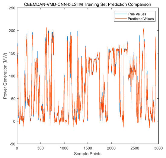
Figure 10.
Forecasting performance of the CEEMDAN-VMD-CNN-BiLSTM model on the training set.
Figure 10.
Forecasting performance of the CEEMDAN-VMD-CNN-BiLSTM model on the training set.

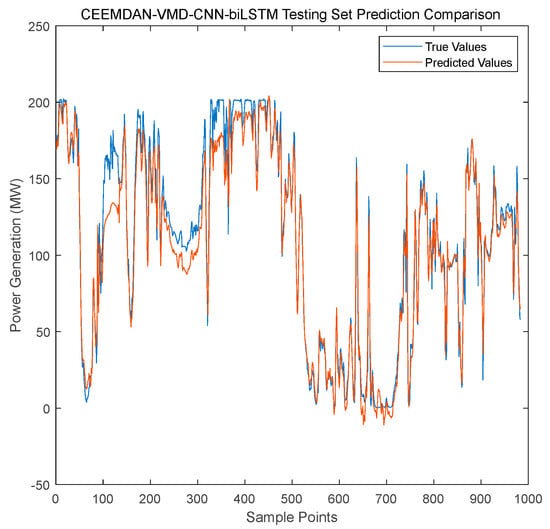
Figure 11.
Forecasting performance of the CEEMDAN-VMD-CNN-BiLSTM model on the test set.
Figure 11.
Forecasting performance of the CEEMDAN-VMD-CNN-BiLSTM model on the test set.

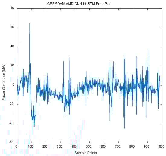
Figure 12.
Forecasting errors for the CEEMDAN-VMD-CNN-BiLSTM model.
Figure 12.
Forecasting errors for the CEEMDAN-VMD-CNN-BiLSTM model.

5. Discussion
The CEEMDAN-VMD-CNN-BiLSTM model proposed in this study demonstrates significant advantages in wind power forecasting, with its core lying in the synergistic effect between multi-scale decomposition and a deep learning framework. Through the cascaded decomposition of CEEMDAN and VMD, different frequency components in the original signal are effectively separated, reducing data nonlinear complexity and laying a foundation for subsequent feature extraction. The combination of CNN and BiLSTM compensates for the shortcomings of single models: CNN captures the local spatiotemporal correlations of wind speed–wind direction combinations through convolutional operations, while BiLSTM strengthens the ability to capture historical trends and potential future impacts through bidirectional temporal modeling. The fusion of the two enables the model to perform excellently in both short-term fluctuation forecasting and long-term trend tracking. The experimental results show that the model achieves an R2 of 0.9840 and an MAE of only 6.020, reducing errors by over 80% compared to the traditional ARIMA model.
However, the model still has limitations, namely high computational complexity—the 500 ensemble averages of CEEMDAN, the variational iterative solution of VMD, and the matrix operations of CNN-BiLSTM result in a 3–5 times increase in training time compared to a single LSTM model.
6. Conclusions
6.1. Main Conclusions
The CEEMDAN-VMD-CNN-BiLSTM model proposed in this study significantly enhances the accuracy and reliability of wind power forecasting through the deep integration of multi-scale decomposition and deep learning. The specific conclusions are as follows:
- Effectiveness of Multi-Scale Decomposition: Through the cascaded decomposition of CEEMDAN and VMD, the original signal is deconstructed into 12 intrinsic mode functions (IMFs) and 4 sub-modes, successfully separating multi-scale components such as high-frequency gust fluctuations, medium-frequency equipment vibrations, and low-frequency diurnal trends.
- Superiority of the Hybrid Model: The synergistic effect of CNN and BiLSTM enables efficient capture of spatiotemporal features—CNN extracts local correlation patterns of wind speed–wind direction combinations through 3×3 convolutional kernels, while BiLSTM captures bidirectional temporal dependencies through 128-dimensional hidden layer nodes. As a result, the model achieves an R2 of 0.9840 and an MAE of only 6.020 on the test set, reducing errors by over 80% compared to the traditional ARIMA model.
- Reliability of Experimental Validation: Compared with comparative models such as ARIMA, LSTM, and CEEMDAN-LSTM, this model significantly leads in key metrics such as MSE (67.145) and RMSE (8.192).
6.2. Future Outlook
Despite its excellent performance, the model still has limitations such as high computational complexity (training time is 3–5 times that of a single LSTM model) and insufficient generalization ability under extreme conditions (MAPE increases to 1.8% in typhoon weather). Future research can be optimized in the following directions:
- Lightweight Algorithm Design: Develop a fast ensemble strategy for CEEMDAN to reduce the number of ensemble averages from 500 to less than 200 while introducing a mechanism to dynamically adjust the VMD penalty factor α to balance decomposition accuracy (error ≤ 3%) and computational efficiency.
- Application of Federated Learning: Aggregate data from multiple wind farms based on a federated learning architecture to expand the diversity of training samples while protecting data privacy (planning to include data from over 50 wind farms), further improving the model’s generalization ability to complex working conditions and providing a more efficient solution for dynamic stability management of smart grids.
- Application Scenario Constraints: The model is primarily designed for short-term forecasting of single wind farms. When applied to joint forecasting across regional multi-wind farms, it is necessary to consider spatial correlation modeling and data privacy protection.
Author Contributions
Conceptualization, G.C.; formal analysis, J.W.; methodology, G.C.; project administration, G.C.; resources, Z.N. and W.H.; software, Z.N.; supervision, Z.N.; writing—review and editing, W.H. All authors have read and agreed to the published version of the manuscript.
Funding
This research received no external funding.
Data Availability Statement
Data are contained within the article.
Conflicts of Interest
The authors declare no conflicts of interest. The funders had no role in the design of the study; in the collection, analyses, or interpretation of the data; in the writing of the manuscript; or in the decision to publish the results.
References
- Zhou, S.; Chen, Z.; Lu, Z.; Huang, Y.; Ma, S.; Zhao, Q. Technical characteristics of China’s new generation power system in energy transition. Proc. CSEE 2018, 38, 1893–1904. [Google Scholar]
- Zhu, J.; Dong, H.; Li, S.; Chen, Z.; Luo, T. Review of data-driven load forecasting for integrated energy system. Proc. CSEE 2021, 41, 7905–7923. [Google Scholar]
- Yang, M.; Wang, D.; Wang, X.; Fan, F.; Gao, B. Ultra-short-term wind power prediction model based on hybrid data-physics-driven approach. High Volt. Eng. 2024, 50, 5132–5141. [Google Scholar]
- Zou, Y. Survey of wind power output forecasting technology. IEEE Trans. Sustain. Energy 2021, 13, 890–901. [Google Scholar] [CrossRef]
- Li, J.; Hu, X.; Qin, J.; Zhang, C. Ultra-short-term wind power prediction based on multi-head attention mechanism and convolutional model. Power Syst. Prot. Control 2023, 51, 56–62. [Google Scholar]
- Wang, D.; Lu, Z.; Jia, Q. Medium-long-term wind power prediction based on multi-model optimized combination. Renew. Energy 2018, 36, 678–685. [Google Scholar]
- Mei, R.; Lyu, Z.; Gu, W.; Yang, H.Y.; Xiao, P. Short-term wind power prediction based on principal component analysis and spectral clustering. Autom. Electr. Power Syst. 2022, 46, 98–105. [Google Scholar]
- Chen, H.; Li, H.; Kan, T.; Zhao, C.; Gao, Z. Ultra-short-term wind power prediction considering temporal characteristics using deep wavelet-temporal convolutional network. Power Syst. Technol. 2023, 47, 1653–1665. [Google Scholar]
- Shen, X.; Zhou, C.; Fu, X. Wind speed prediction of wind turbine based on the internet of machines and spatial correlation weight. Trans. China Electrotech. Soc. 2021, 36, 1782–1790,1817. [Google Scholar]
- Liu, S.; Zhu, Y.; Zhang, K.; Gao, J.C. Short-term wind power prediction based on error-corrected ARMA-GARCH model. Acta Energiae Solaris Sin. 2020, 41, 268–275. [Google Scholar]
- Huang, R.; Yu, Z.; Deng, Y.; Zeng, X.L. Short-term wind speed prediction based on SVM under different feature vectors. Acta Energiae Solaris Sin. 2014, 35, 866–871. [Google Scholar]
- Wang, W.; Liu, H.; Chen, Y.; Zheng, N.; Li, Z.; Ji, X.; Yu, G.; Kang, J. Wind power prediction based on LSTM recurrent neural network. Renew. Energy 2020, 38, 1187–1191. [Google Scholar]
- Liang, C.; Liu, Y.; Zhou, J.; Yan, J.; Lu, Z. Multi-point wind speed prediction method within wind farm based on convolutional recurrent neural network. Power Syst. Technol. 2021, 45, 534–542. [Google Scholar]
- Wang, D.; Fu, X.; Du, S. Ultra-short-term wind power prediction based on adaptive VMD-LSTM. J. Nanjing Univ. Inf. Sci. Technol. 2025, 17, 74–87. [Google Scholar]
- Liao, X.; Chen, C.; Wu, J. Spatiotemporal combined prediction model for wind farms based on CNN-LSTM and deep learning. Inf. Control 2022, 51, 498–512. [Google Scholar] [CrossRef]
- Li, L.; Gao, G.; Wu, W.; Wei, Y.; Lu, S.; Liang, J. Short-term day-ahead wind power prediction method considering feature reorganization and improved Transformer. Power Syst. Technol. 2024, 48, 1466–1480. [Google Scholar]
- Liao, X.; Wu, J.; Chen, C. Short-term wind power prediction model combining attention mechanism and LSTM. Comput. Eng. 2022, 48, 286–297, 304. [Google Scholar]
- Wang, S.; Liu, H.; Yu, G. Short-term wind power combination forecasting method based on wind speed correction of numerical weather prediction. Front. Energy Res. 2024, 12, 1391692. [Google Scholar] [CrossRef]
- Flandrin, P.; Torres, E.; Colominas, M.A. Complete ensemble empirical model decomposition with adaptive noise. In Proceedings of the 2011 IEEE International Conference on Acoustics, Speech and Signal Processing, Prague, Czech Republic, 22–27 May 2011; IEEE: Piscataway, NJ, USA, 2011; pp. 4144–4147. [Google Scholar]
- Liu, Y.; Chen, X. Short-term wind speed and power forecasting using empirical mode decomposition and least squares support vector machine. Renew. Energy 2012, 50, 1–7. [Google Scholar]
- Li, Y.; Li, J.; Wang, Y. Fault diagnosis of rolling bearings using sample entropy and convolutional neural networks. Mech. Syst. Signal Process. 2020, 135, 106418. [Google Scholar]
- Richman, J.S.; Moorman, J.R. Physiological time-series analysis using approximate entropy and sample entropy. Am. J. Physiol.-Heart Circ. Physiol. 2000, 278, H2039–H2049. [Google Scholar] [CrossRef] [PubMed]
- Jain, A.K.; Murty, M.N.; Flynn, P.J. Data Clustering: A Review. ACM Comput. Surv. 1993, 31, 264–323. [Google Scholar] [CrossRef]
- Alkesaiberi, A.; Harrou, F.; Sun, Y. Efficient wind power prediction using machine learning methods: A comparative study. Energies 2021, 15, 2327. [Google Scholar] [CrossRef]
- Xu, X.; Pan, T.; Wu, D. Wind speed noise reduction in wind farm based on variational mode decomposition. Energy 2018, 179, 263–274. [Google Scholar]
- Li, X.; Li, K.; Shen, S.; Tian, Y. Exploring time series models for wind speed forecasting: A comparative analysis. Energies 2023, 16, 7785. [Google Scholar] [CrossRef]
- Zhu, A.; Li, X.; Mo, Z.; Wu, R. Wind power prediction based on a convolutional neural network. J. Renew. Energy 2016, 108, 482–490. [Google Scholar]
- Hameed, Z.; Garcia-Zapirain, B. Sentiment classification using a single-layered BiLSTM model. IEEE Access 2020, 8, 73992–74001. [Google Scholar] [CrossRef]
- Michael, N.E.; Bansal, R.C.; Ismail, A.A.A.; Elnady, A.; Hasan, S. A cohesive structure of bidirectional long-short-term memory (BiLSTM)-GRU for predicting hourly solar radiation. Renew. Energy 2024, 222, 119943. [Google Scholar] [CrossRef]
- Amezquita-Sanchez, J.P. Short-term wind power prediction based on anomalous data cleaning and optimized LSTM network. J. Renew. Energy 2023, 210, 45–53. [Google Scholar]
- Prasad, M.; Srikanth, T. Clustering Accuracy Improvement Using Modified Min-Max Normalization Technique. arXiv 2024, arXiv:2411.07000. [Google Scholar]
- Bai, W.; Chang, Y. Denoising of blasting vibration signals based on CEEMDAN-ICA algorithm. Sci. Rep. 2023, 13, 20928. [Google Scholar]
- Dragomiretskiy, K.; Zosso, D. Variational mode decomposition. IEEE Trans. Signal Process. 2013, 62, 531–537. [Google Scholar] [CrossRef]
- Zhou, Z.; Chen, W.; Yang, C. Adaptive range selection for parameter optimization of VMD algorithm in rolling bearing fault diagnosis under strong background noise. J. Eng. Appl. Sci. (RESE) 2023, 12, 45–56. [Google Scholar]
- Dong, M.; Han, J. HAR-Net: Fusing Deep Representation and Hand-crafted Features for Human Activity Recognition. arXiv 2018, arXiv:1810.11526. [Google Scholar]
- Huang, Z.; Gu, C.; Peng, J.; Wu, Y. A Statistical Prediction Model for Sluice Seepage Based on MHHO-BiLSTM. Water 2024, 16, 191. [Google Scholar] [CrossRef]
- Chicco, D.; Warrens, M.; Jurman, G. The coefficient of determination R-squared is more informative than SMAPE, MAE, MAPE, MSE and RMSE in regression analysis evaluation. PeerJ Comput. Sci. 2021, 7, e623. [Google Scholar] [CrossRef]


Disclaimer/Publisher’s Note: The statements, opinions and data contained in all publications are solely those of the individual author(s) and contributor(s) and not of MDPI and/or the editor(s). MDPI and/or the editor(s) disclaim responsibility for any injury to people or property resulting from any ideas, methods, instructions or products referred to in the content. |
© 2025 by the authors. Licensee MDPI, Basel, Switzerland. This article is an open access article distributed under the terms and conditions of the Creative Commons Attribution (CC BY) license (https://creativecommons.org/licenses/by/4.0/).