
DC Microgrid Enhancement via Chaos Game Optimization Algorithm

 ,
,  , , ,
, , ,  and
and
Abstract
1. Introduction
2. Materials and Methods
2.1. DGUS System
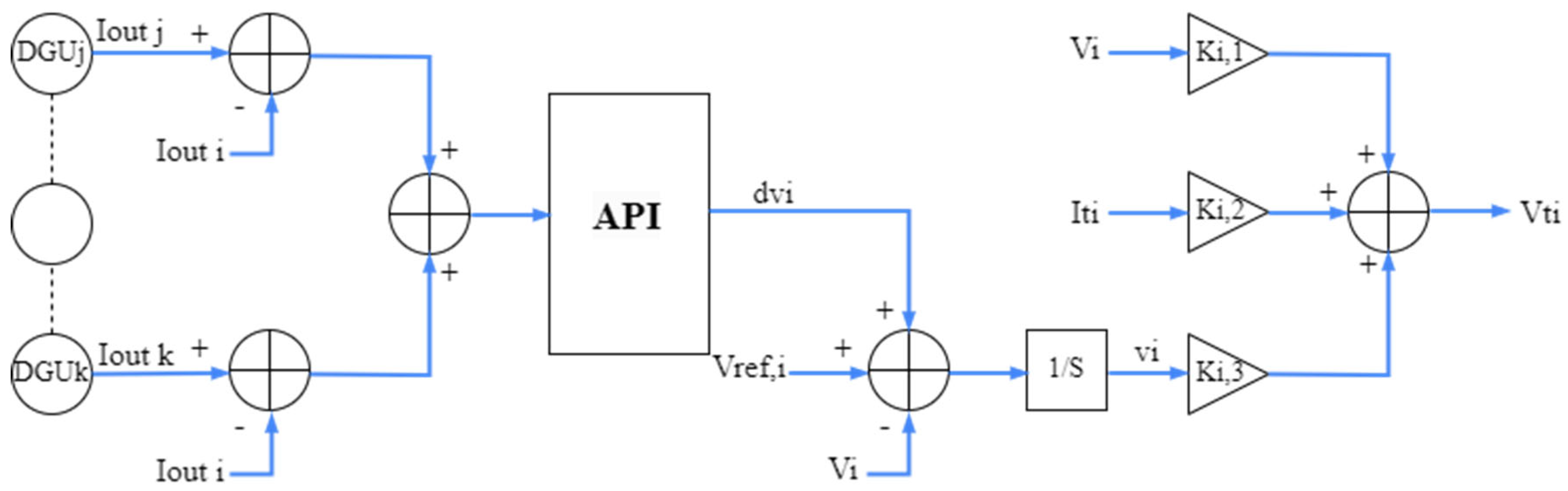
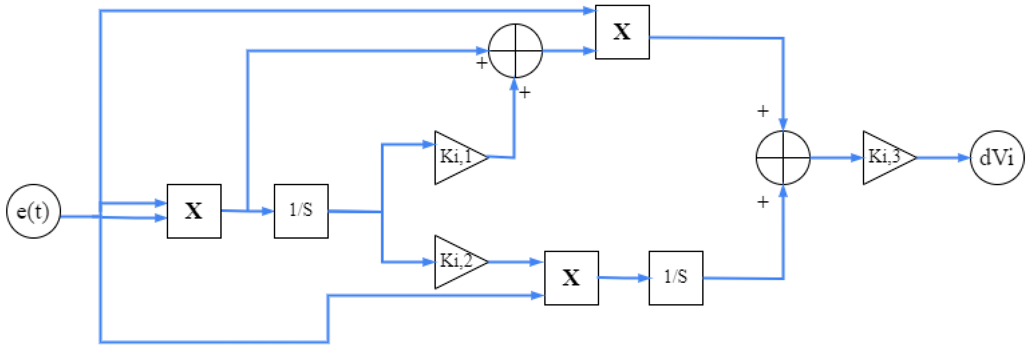
2.1.1. Primary Control Layer
2.1.2. Secondary Control Layer
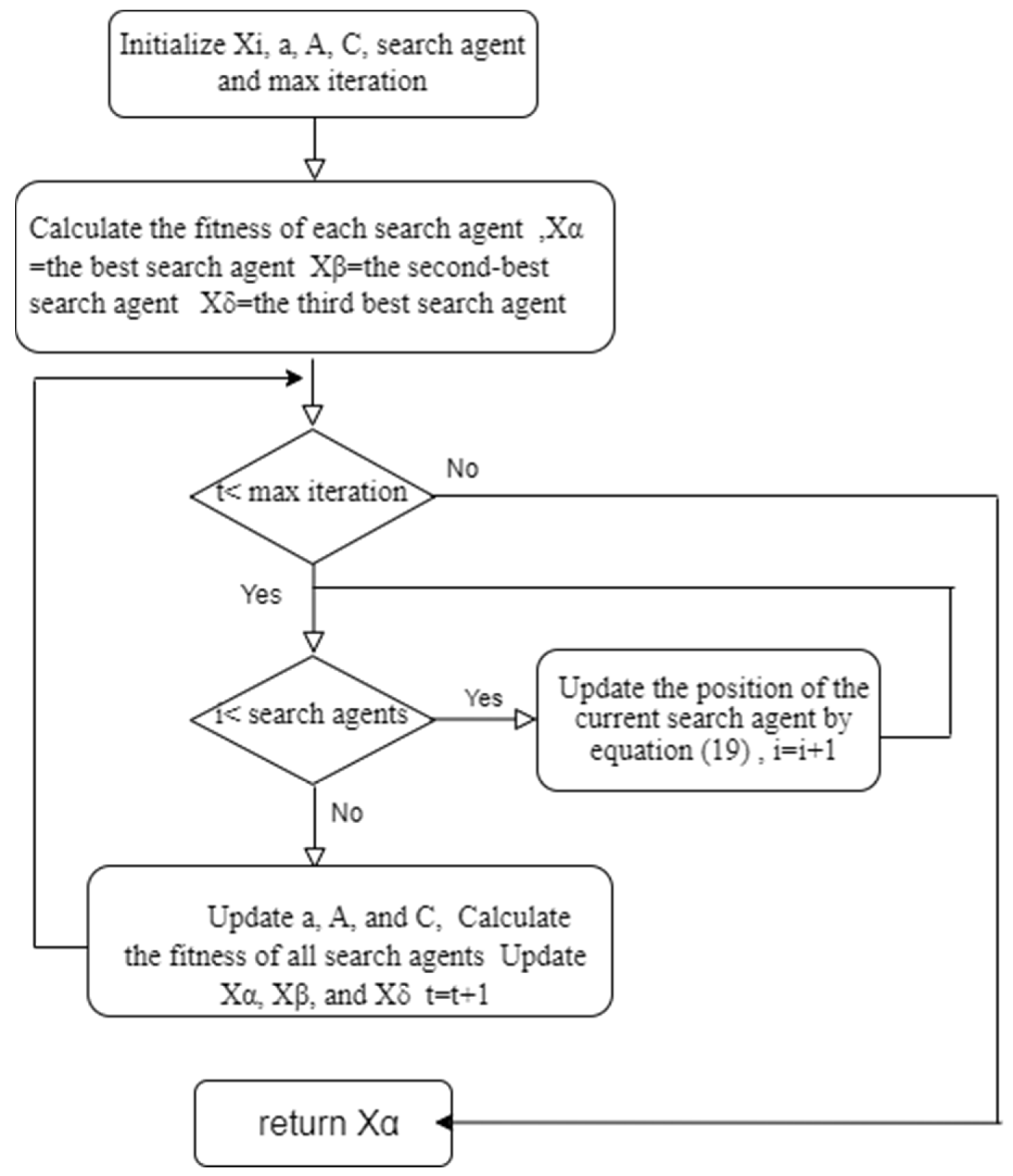
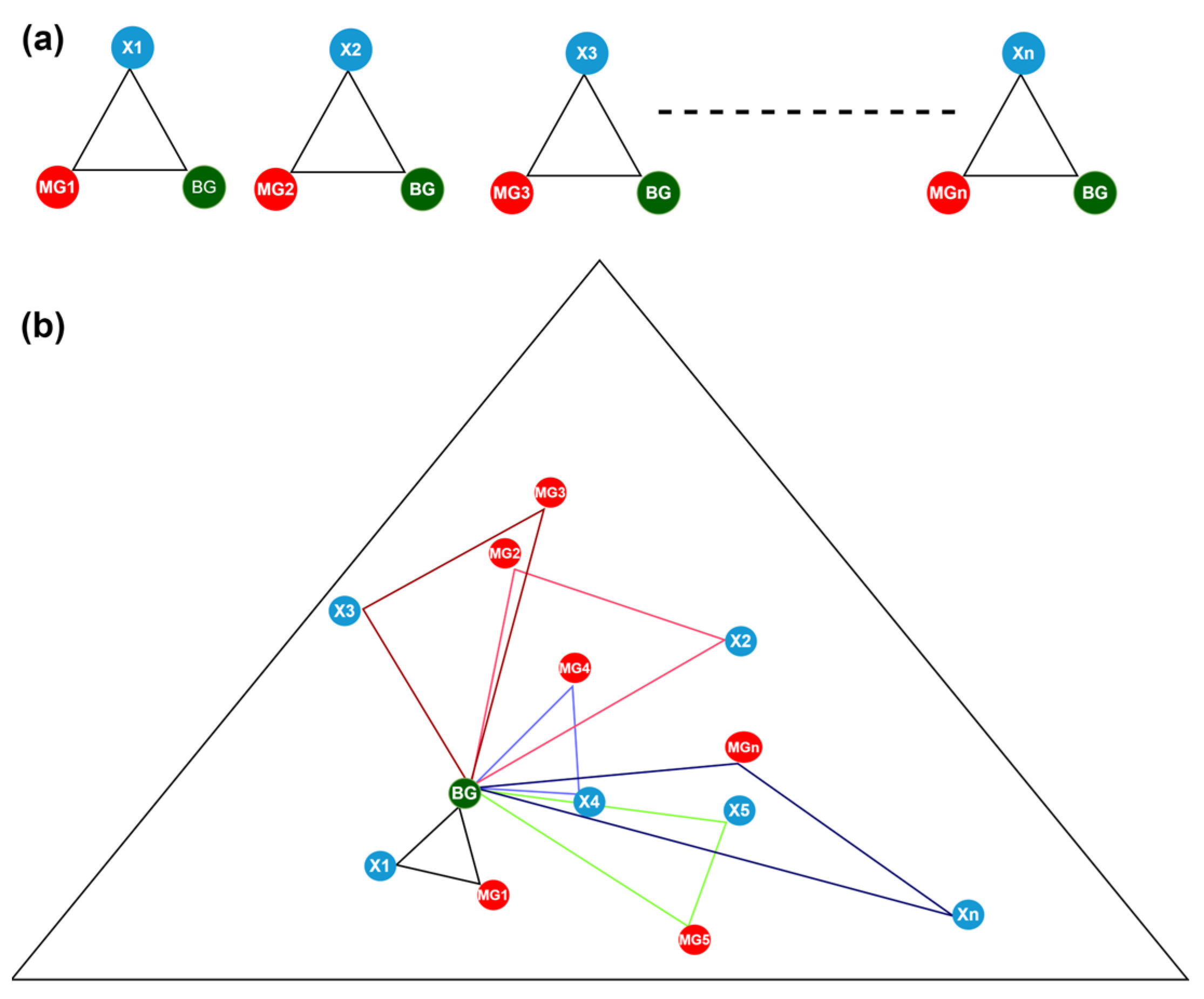
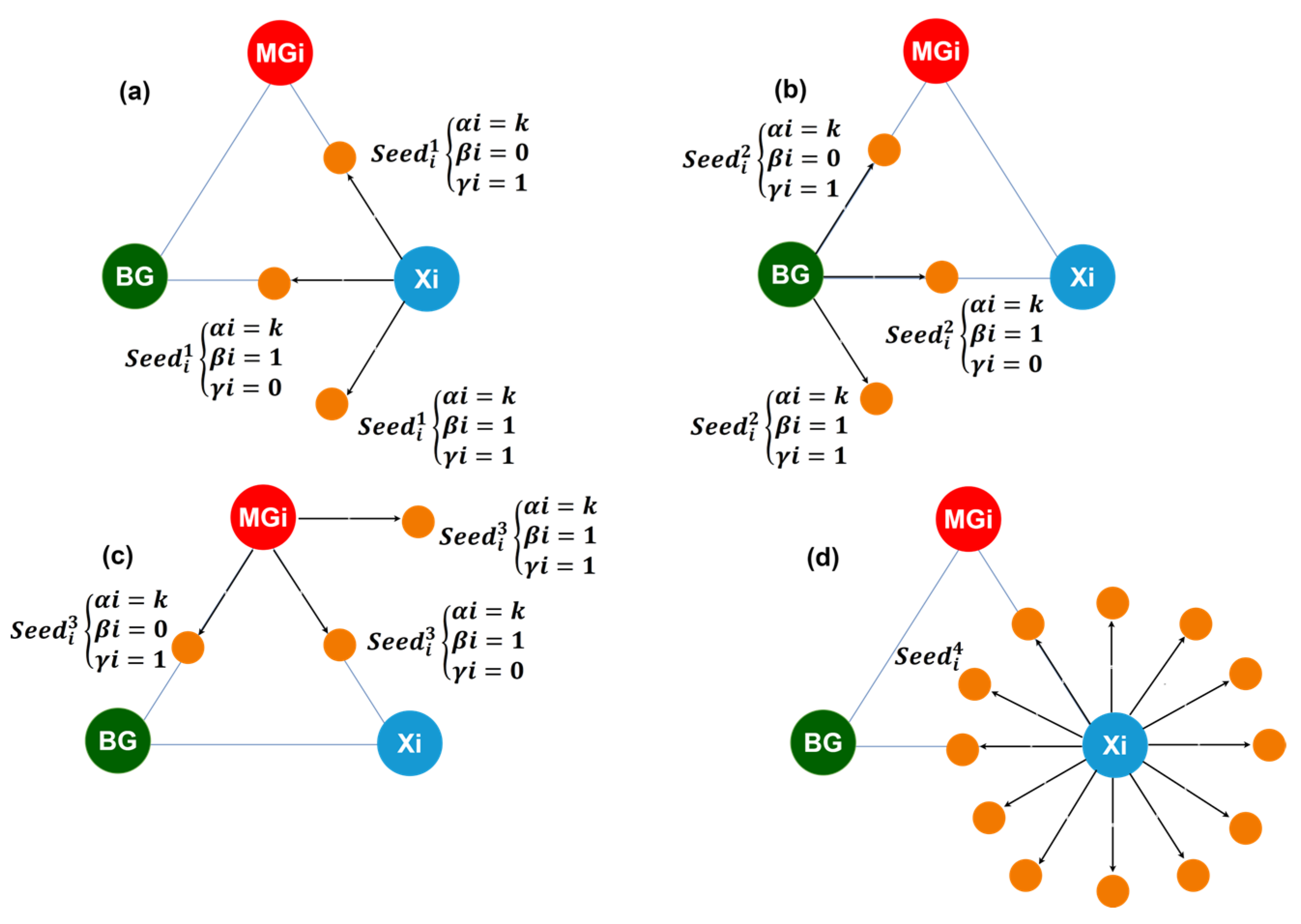
2.2. Optimization Tools
- The position of the so far found global best (GB).
- The position of the mean group (MGi).
- The position of the ith solution candidate (Xi) as the selected seed.
3. Results
4. Discussion
5. Conclusions
Author Contributions
Funding
Data Availability Statement
Conflicts of Interest
References
- Ashok Kumar, A.; Amutha Prabha, N. A comprehensive review of DC microgrid in market segments and control technique. Heliyon 2022, 8, e11694. [Google Scholar] [CrossRef] [PubMed]
- Al-Kahtani, M.S.; Karim, L. A Survey on Attacks and Defense Mechanisms in Smart Grids. Int. J. Comput. Eng. Inf. Technol. 2019, 11, 94–100. [Google Scholar]
- Banerji, A.; Sen, D.; Bera, A.K.; Ray, D.; Paul, D.; Bhakat, A.; Biswas, S.K. Microgrid: A Review. In Proceedings of the 2013 IEEE Global Humanitarian Technology Conference: South Asia Satellite (GHTC-SAS), Trivandrum, India, 23–24 August 2013; pp. 27–35. [Google Scholar] [CrossRef]
- Zhang, Z.; Gong, S.; Dimitrovski, A.D.; Li, H. Time Synchronization Attack in Smart Grid: Impact and Analysis. IEEE Trans. Smart Grid 2013, 4, 87–98. [Google Scholar] [CrossRef]
- Khoei, T.T.; Ould Slimane, H.; Kaabouch, N. A Comprehensive Survey on the Cyber-Security of Smart Grids: Cyber-Attacks, Detection, Countermeasure Techniques, and Future Directions. arXiv 2022, arXiv:2207.07738. [Google Scholar]
- Yakout, A.H.; AboRas, K.M.; Kotb, H.; Alharbi, M.; Shouran, M.; Abdul Samad, B. A Novel Ultra Local Based-Fuzzy PIDF Controller for Frequency Regulation of a Hybrid Microgrid System with High Renewable Energy Penetration and Storage Devices. Processes 2023, 11, 1093. [Google Scholar] [CrossRef]
- Yakout, A.H.; Hasanien, H.M.; Turky, R.A.; Abu-Elanien, A.E.B. Improved reinforcement learning strategy of energy storage units for frequency control of hybrid power systems. J. Energy Storage 2023, 72, 108248. [Google Scholar] [CrossRef]
- Llaria, A.; Dos Santos, J.; Terrasson, G.; Boussaada, Z.; Merlo, C.; Curea, O. Intelligent Buildings in Smart Grids: A Survey on Security and Privacy Issues Related to Energy Management. Energies 2021, 14, 2733. [Google Scholar] [CrossRef]
- Danda, B.R.; Chandra, B. Cyber Security for Smart Grid Systems: Status, Challenges and Perspectives; Institute of Electrical and Electronics Engineers: New York, NY, USA, 2015. [Google Scholar] [CrossRef]
- Al-Ismail, F.S. DC Microgrid Planning, Operation, and Control: A Comprehensive Review. IEEE Access 2021, 9, 36154–36172. [Google Scholar] [CrossRef]
- Li, D.; Ho, C.N.M. A Module-Based Plug-n-Play DC Microgrid with Fully Decentralized Control for IEEE Empower a Billion Lives Competition. IEEE Trans. Power Electron. 2021, 36, 1764–1776. [Google Scholar] [CrossRef]
- Pullaguram, D.; Mishra, S.; Senroy, N. Event-Triggered Communication Based Distributed Control Scheme for DC Microgrid. IEEE Trans. Power Syst. 2018, 33, 5583–5593. [Google Scholar] [CrossRef]
- Kumar, J.; Agarwal, A.; Agarwal, V. A review on overall control of DC microgrids. J. Energy Storage 2019, 21, 113–138. [Google Scholar] [CrossRef]
- Yamashita, D.Y.; Vechiu, I.; Gaubert, J.-P. A review of hierarchical control for building microgrids. Renew. Sustain. Energy Rev. 2020, 118, 109523. [Google Scholar] [CrossRef]
- Olivares, D.E.; Mehrizi-Sani, A.; Etemadi, A.H.; Cañizares, C.A.; Iravani, R.; Kazerani, M.; Hajimiragha, A.H.; Gomis-Bellmunt, O.; Saeedifard, M.; Palma-Behnke, R.; et al. Trends in Microgrid Control. IEEE Trans. Smart Grid 2014, 5, 1905–1919. [Google Scholar] [CrossRef]
- Li, X.; Hu, C.; Luo, S.; Lu, H.; Piao, Z.; Jing, L. Distributed Hybrid-Triggered Observer-Based Secondary Control of Multi-Bus DC Microgrids Over Directed Networks. IEEE Trans. Circuits Syst. I Regul. Pap. 2025, 72, 2467–2480. [Google Scholar] [CrossRef]
- Yang, N.; Xu, G.; Fei, Z.; Li, Z.; Du, L.; Guerrero, J.M.; Huang, Y.; Yan, J.; Xing, C.; Li, Z. Two-Stage Coordinated Robust Planning of Multi-Energy Ship Microgrids Considering Thermal Inertia and Ship Navigation. IEEE Trans. Smart Grid 2025, 16, 1100–1111. [Google Scholar] [CrossRef]
- Bidram, A.; Davoudi, A. Hierarchical Structure of Microgrids Control System. IEEE Trans. Smart Grid 2012, 3, 1963–1976. [Google Scholar] [CrossRef]
- Mirjalili, S. SCA: A Sine Cosine Algorithm for solving optimization problems. Knowl. Based Syst. 2016, 96, 120–133. [Google Scholar] [CrossRef]
- Mirjalili, S.; Lewis, A. The Whale Optimization Algorithm. Adv. Eng. Softw. 2016, 95, 51–67. [Google Scholar] [CrossRef]
- Talatahari, S.; Azizi, M. Chaos Game Optimization: A novel metaheuristic algorithm. Artif. Intell. Rev. 2021, 54, 917–1004. [Google Scholar] [CrossRef]
- Mirjalili, S.; Mirjalili, S.M.; Lewis, A. Grey Wolf Optimizer. Adv. Eng. Softw. 2014, 69, 46–61. [Google Scholar] [CrossRef]
- Mirjalili, S.; Gandomi, A.H.; Mirjalili, S.Z.; Saremi, S.; Faris, H.; Mirjalili, S.M. Salp Swarm Algorithm: A bio-inspired optimizer for engineering design problems. Adv. Eng. Softw. 2017, 114, 163–191. [Google Scholar] [CrossRef]
- Xue, J.; Shen, B. Dung beetle optimizer: A new meta-heuristic algorithm for global optimization. J. Supercomput. 2023, 79, 7305–7336. [Google Scholar] [CrossRef]
- Riverso, S.; Sarzo, F.; Ferrari-Trecate, G. Plug-and-Play Voltage and Frequency Control of Islanded Microgrids with Meshed Topology. IEEE Trans. Smart Grid 2015, 6, 1176–1184. [Google Scholar] [CrossRef]
- El-Ebiary, A.H.; Mokhtar, M.; Attia, M.A.; Marei, M.I. A Distributed Adaptive Control Strategy for Meshed DC Microgrids. In Proceedings of the 2023 IEEE Conference on Power Electronics and Renewable Energy (CPERE), Luxor, Egypt, 19–21 February 2023; pp. 1–6. [Google Scholar] [CrossRef]
- Khader, A.H.; Yakout, A.H.; El-Sharkawy, M. Damping Interarea Oscillations Using PID Power System Stabilizer with Grey Wolf Algorithm and Particle Swarm Algorithm. In Proceedings of the 2019 21st International Middle East Power Systems Conference (MEPCON), Cairo, Egypt, 17–19 December 2019; pp. 330–336. [Google Scholar] [CrossRef]
- Mosaad, A.M.; Attia, M.A.; Abdelaziz, A.Y. Whale optimization algorithm to tune PID and PIDA controllers on AVR system. Ain Shams Eng. J. 2019, 10, 755–767. [Google Scholar] [CrossRef]
- Tucci, M.; Riverso, S.; Vasquez, J.C.; Guerrero, J.M.; Ferrari-Trecate, G. A Decentralized Scalable Approach to Voltage Control of DC Islanded Microgrids. IEEE Trans. Control Syst. Technol. 2016, 24, 1965–1979. [Google Scholar] [CrossRef]
- Riverso, S.; Farina, M.; Ferrari-Trecate, G. Plug-and-play model predictive control based on robust control invariant sets. Automatica 2014, 50, 2179–2186. [Google Scholar] [CrossRef]
- Yuan, M.; Fu, Y.; Mi, Y.; Li, Z.; Wang, C. Hierarchical control of DC microgrid with dynamical load power sharing. Appl. Energy 2019, 239, 1–11. [Google Scholar] [CrossRef]
- El-Ebiary, A.H.; Attia, M.A.; Awad, F.H.; Marei, M.I.; Mokhtar, M. Kalman Filters Based Distributed Cyber-Attack Mitigation Layers for DC Microgrids. IEEE Trans. Circuits Syst. I Regul. Pap. 2024, 71, 1358–1370. [Google Scholar] [CrossRef]
- EL-Ebiary, A.H.; Mokhtar, M.; Mansour, A.M.; Awad, F.H.; Marei, M.I.; Attia, M.A. Distributed Mitigation Layers for Voltages and Currents Cyber-Attacks on DC Microgrids Interfacing Converters. Energies 2022, 15, 9426. [Google Scholar] [CrossRef]
- Lofberg, J. YALMIP: A Toolbox for Modeling and Optimization in MATLAB. In Proceedings of the 2004 IEEE International Conference on Robotics and Automation (IEEE Cat. No.04CH37508), Taipei, Taiwan, 2–4 September 2004; pp. 284–289. [Google Scholar] [CrossRef]
- Choi, K.; Liu, H. Matlab and Simulink Basics. In Problem-Based Learning in Communication Systems Using Matlab and Simulink; Wiley: Hoboken, NJ, USA, 2016; pp. 1–15. [Google Scholar] [CrossRef]
- Olfati-Saber, R.; Murray, R.M. Consensus Problems in Networks of Agents with Switching Topology and Time-Delays. IEEE Trans. Autom. Contr. 2004, 49, 1520–1533. [Google Scholar] [CrossRef]
- Mokhtar, M.; Marei, M.I.; El-Sattar, A.A. Improved Current Sharing Techniques for DC Microgrids. Electr. Power Compon. Syst. 2018, 46, 757–767. [Google Scholar] [CrossRef]
- Qais, M.H.; Hasanien, H.M.; Turky, R.A.; Alghuwainem, S.; Tostado-Véliz, M.; Jurado, F. Circle Search Algorithm: A Geometry-Based Metaheuristic Optimization Algorithm. Mathematics 2022, 10, 1626. [Google Scholar] [CrossRef]
- Heidari, A.A.; Mirjalili, S.; Faris, H.; Aljarah, I.; Mafarja, M.; Chen, H. Harris hawks optimization: Algorithm and applications. Future Gener. Comput. Syst. 2019, 97, 849–872. [Google Scholar] [CrossRef]
- Qais, M.H.; Hasanien, H.M.; Alghuwainem, S. Output power smoothing of grid-connected permanent-magnet synchronous generator driven directly by variable speed wind turbine: A review. J. Eng. 2017, 2017, 1755–1759. [Google Scholar] [CrossRef]
- Qais, M.H.; Hasanien, H.M.; Alghuwainem, S. Transient search optimization: A new meta-heuristic optimization algorithm. Appl. Intell. 2020, 50, 3926–3941. [Google Scholar] [CrossRef]
- Mech, L.D. Alpha Status, Dominance, and Division of Labor in Wolf Packs. 1999. Available online: https://digitalcommons.unl.edu/usgsnpwrc/353 (accessed on 24 June 2025).
- Muro, C.; Escobedo, R.; Spector, L.; Coppinger, R.P. Wolf-pack (Canis lupus) hunting strategies emerge from simple rules in computational simulations. Behav. Process. 2011, 88, 192–197. [Google Scholar] [CrossRef]
- Dahou, A.; Chelloug, S.A.; Alduailij, M.; Elaziz, M.A. Improved Feature Selection Based on Chaos Game Optimization for Social Internet of Things with a Novel Deep Learning Model. Mathematics 2023, 11, 1032. [Google Scholar] [CrossRef]


| Primary Control Gain Ki | |
|---|---|
| DGU i | Ki |
| DGU 1 | K1 = [−2.31, −0.16, 13.55] |
| DGU 2 | K2 = [−0.87, −0.05, 48.28] |
| DGU 3 | K3 = [−0.48, −0.108, 30.67] |
| DGU 4 | K4 = [−7, −0.175, 102.96] |
| Sudden Local Load RL [Ohm] | |
|---|---|
| DGU 1 | RL = 20 ohms |
| DGU 2 | RL = 18 ohms |
| DGU 3 | RL = 16 ohms |
| DGU 4 | RL = 14 ohms |
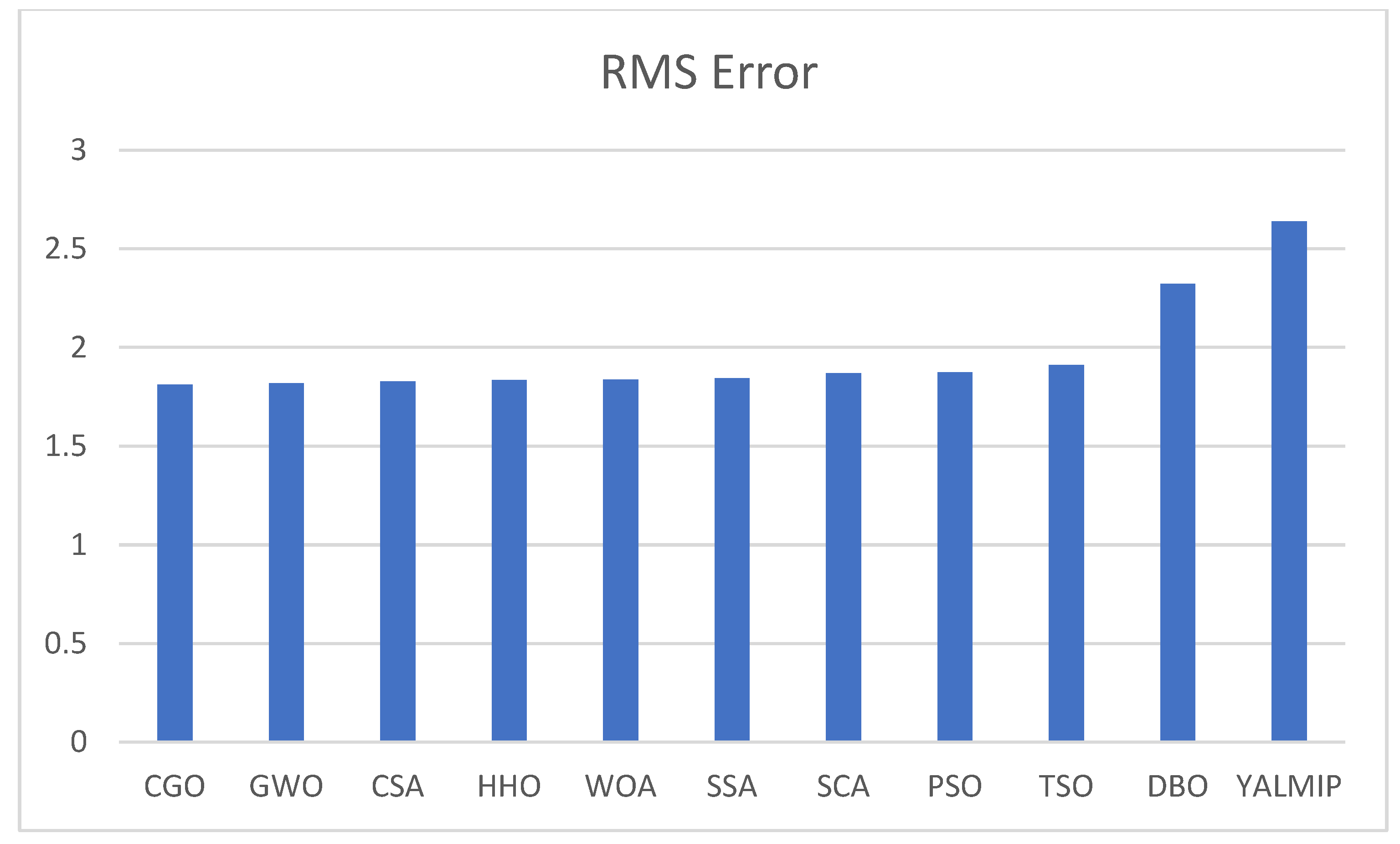
| Algorithm | K1 | K2 | k3 | RMS Error | Searching Time (sec) |
|---|---|---|---|---|---|
| CGO | 0.9714 | 0.0081 | 1.0000 | 1.8117 | 427,161 |
| GWO | 0.9288 | 0.0121 | 0.7139 | 1.8187 | 98,888 |
| CSA | 0.9501 | 0.0186 | 0.4384 | 1.8301 | 117,855 |
| HHO | 0.9295 | 0.0227 | 0.3997 | 1.8348 | 227,608 |
| WOA | 1.0000 | 0.0243 | 0.3497 | 1.8360 | 99,480 |
| SSA | 0.8979 | 0.0209 | 0.6652 | 1.8433 | 230,876 |
| SCA | 0.9705 | 0.0348 | 0.3962 | 1.8694 | 235,628 |
| PSO | 0.9972 | 0.0000 | 0.9825 | 1.8738 | 109,531 |
| TSO | 0.9949 | 0.0587 | 0.1705 | 1.9120 | 103,917 |
| DBO | 0.9037 | 0.0597 | 0.3933 | 2.3214 | 335,267 |
| YALMIP | 1 | 0.8 | 0.9 | 2.6386 |
| Algorithm | RMS Error Repeated Results (10 Times) | Std. Dev. | Minimum | Mean | t-Test | ||||
|---|---|---|---|---|---|---|---|---|---|
| CGO | 1.8772 | 1.8240 | 1.8135 | 1.8117 | 1.8117 | 0.020578 | 1.8117 | 1.819557 | - |
| 1.8117 | 1.8117 | 1.8117 | 1.8117 | 1.8117 | |||||
| GWO | 1.9975 | 1.9803 | 1.8663 | 1.8248 | 1.8248 | 0.070156 | 1.8187 | 1.857706 | 0.052429 |
| 1.8191 | 1.8191 | 1.8191 | 1.8189 | 1.8187 | |||||
| CSA | 1.8515 | 1.8433 | 1.8433 | 1.8373 | 1.8369 | 0.008196 | 1.8278 | 1.835744 | 8.08 × 10⁻⁷ |
| 1.8322 | 1.8297 | 1.8278 | 1.8278 | 1.8278 | |||||
| HHO | 1.9975 | 1.8510 | 1.8418 | 1.8369 | 1.8369 | 0.050524 | 1.8348 | 1.853767 | 2.33 × 10⁻¹¹ |
| 1.8369 | 1.8364 | 1.8361 | 1.8353 | 1.8348 | |||||
| WOA | 1.9975 | 1.9975 | 1.8412 | 1.8412 | 1.8375 | 0.067455 | 1.836 | 1.868511 | 0.016809 |
| 1.8364 | 1.8364 | 1.8360 | 1.8360 | 1.8360 | |||||
| SSA | 1.9975 | 1.9975 | 1.9104 | 1.8869 | 1.8675 | 0.061846 | 1.8433 | 1.887288 | 0.01394 |
| 1.8480 | 1.8437 | 1.8437 | 1.8433 | 1.8433 | |||||
| SCA | 1.9975 | 1.8920 | 1.8920 | 1.8920 | 1.8920 | 0.037298 | 1.8694 | 1.895449 | 2.3 × 10⁻⁸ |
| 1.8920 | 1.8920 | 1.8694 | 1.8694 | 1.8694 | |||||
| PSO | 1.9066 | 1.8844 | 1.8844 | 1.8738 | 1.8738 | 0.010588 | 1.8738 | 1.879173 | 0.02222 |
| 1.8738 | 1.8738 | 1.8738 | 1.8738 | 1.8738 | |||||
| TSO | 1.9975 | 1.9143 | 1.9143 | 1.9143 | 1.9143 | 0.026575 | 1.912 | 1.921768 | 4.41 × 10⁻¹³ |
| 1.9143 | 1.9143 | 1.9120 | 1.9120 | 1.9120 | |||||
| DBO | 2.7024 | 2.6145 | 2.4315 | 2.3718 | 2.3512 | 0.136239 | 2.3214 | 2.407784 | 2.24 × 10⁻⁷ |
| 2.3508 | 2.3245 | 2.3214 | 2.3214 | 2.3214 | |||||
| Algorithms | Specific Parameters | Value |
|---|---|---|
| CGO | α | Random 1 to 4 |
| β | Random 1 to 2 | |
| γ | Random 1 to 2 | |
| GWO | a1 | Random 2 to 0 |
| r1 | Random 0 to 1 | |
| r2 | Random 0 to 1 | |
| CSA | c | 0.8 |
| p | 0.991 | |
| HHO | r1, r2, r3, and r4 | Random 0 to 1 |
| q | Random 0 to 1 | |
| E1 | Random 2 to 0 | |
| E0 | Random −2 to 0 | |
| WOA | r1 and r2 | Random 0 to 1 |
| a | Random 0 to 2 | |
| b | 1 | |
| p | Random 0 to 1 | |
| SSA | c1 | 1 to 1.054 |
| c2 and c3 | Random 0 to 1 | |
| s | 1 | |
| SCA | r1 | Random 2 to 0 |
| r2 | Random 0 to 2π | |
| r3 and r4 | Random 0 to 1 | |
| t | 2 | |
| a | 2 | |
| PSO | w1 | 0.5 to 0.3 |
| c1 | 2 | |
| c2 | 2 | |
| TSO | r1, r2, and r3 | Random 0 to 1 |
| k | 1 | |
| DBO | p | 0.2 |
| a | 1 | |
| r2 | Random 0 to 1 | |
| b1 | 0.3 | |
| b2 | 0.1 |
Disclaimer/Publisher’s Note: The statements, opinions and data contained in all publications are solely those of the individual author(s) and contributor(s) and not of MDPI and/or the editor(s). MDPI and/or the editor(s) disclaim responsibility for any injury to people or property resulting from any ideas, methods, instructions or products referred to in the content. |
© 2025 by the authors. Licensee MDPI, Basel, Switzerland. This article is an open access article distributed under the terms and conditions of the Creative Commons Attribution (CC BY) license (https://creativecommons.org/licenses/by/4.0/).
Share and Cite
Heikal, A.S.; Diaaeldin, I.M.; Badra, N.M.; Attia, M.A.; Badr, A.O.; Omar, O.A.M.; EL-Ebiary, A.H.; Kang, H.-S. DC Microgrid Enhancement via Chaos Game Optimization Algorithm. Processes 2025, 13, 2042. https://doi.org/10.3390/pr13072042
Heikal AS, Diaaeldin IM, Badra NM, Attia MA, Badr AO, Omar OAM, EL-Ebiary AH, Kang H-S. DC Microgrid Enhancement via Chaos Game Optimization Algorithm. Processes. 2025; 13(7):2042. https://doi.org/10.3390/pr13072042
Chicago/Turabian StyleHeikal, Abdelrahman S., Ibrahim Mohamed Diaaeldin, Niveen M. Badra, Mahmoud A. Attia, Ahmed O. Badr, Othman A. M. Omar, Ahmed H. EL-Ebiary, and Hyun-Soo Kang. 2025. "DC Microgrid Enhancement via Chaos Game Optimization Algorithm" Processes 13, no. 7: 2042. https://doi.org/10.3390/pr13072042
APA StyleHeikal, A. S., Diaaeldin, I. M., Badra, N. M., Attia, M. A., Badr, A. O., Omar, O. A. M., EL-Ebiary, A. H., & Kang, H.-S. (2025). DC Microgrid Enhancement via Chaos Game Optimization Algorithm. Processes, 13(7), 2042. https://doi.org/10.3390/pr13072042