EECNet: An Efficient Edge Computing Network for Transmission Line Ice Thickness Recognition

Abstract

The recognition of ice thickness on transmission lines serves as a prerequisite for controlling de-icing robots to carry out precise de-icing operations. To address the issue that existing edge computing terminals fail to meet the demands of ice thickness recognition algorithms, this paper introduces an Efficient Edge Computing Network (EECNet) specifically designed for identifying ice thickness on transmission lines. Firstly, pruning is applied to the Efficient Neural Network (ENet), removing redundant components within the encoder to decrease both the computational complexity and the number of parameters in the model. Secondly, a Dilated Asymmetric Bottleneck Module (DABM) is proposed. By integrating different types of convolutions, this module effectively strengthens the model’s capability to extract features from ice-covered transmission lines. Then, an Efficient Partial Conv Module (EPCM) is designed, introducing an adaptive partial convolution selection mechanism that innovatively combines attention mechanisms with partial convolutions. This design enhances the model’s ability to select important feature channels. The method involves segmenting ice-covered images to obtain iced regions and then calculating the ice thickness using the iced area and known cable parameters. Experimental validation on an ice-covered transmission line dataset shows that EECNet achieves a segmentation accuracy of 92.7% in terms of the Mean Intersection over Union (mIoU) and an F1-Score of 96.2%, with an ice thickness recognition error below 3.4%. Compared to ENet, the model’s parameter count is reduced by 41.7%, and the detection speed on OrangePi 5 Pro is improved by 27.3%. After INT8 quantization, the detection speed is increased by 26.3%. These results demonstrate that EECNet not only enhances the recognition speed on edge equipment but also maintains high-precision ice thickness recognition.

1. Introduction

Transmission lines are important carriers of power transmission systems. When transmission lines encounter severe weather conditions, such as strong winds and freezing rain, a large amount of ice and snow accumulates on their surfaces, forming ice [1,2]. The ice cover on transmission lines not only significantly increases their weight load, causing sag drop and tower collapse, but also easily leads to serious faults, such as insulator flashover, seriously threatening the stable operation of the entire power system. Therefore, how to efficiently remove the ice on transmission lines is an urgent problem to be solved [3,4,5]. Due to the harsh environment in which power transmission lines are prone to icing, using a de-icing robot to automate resonance de-icing is an effective solution. The accurate recognition of the ice thickness on transmission lines is a prerequisite for automated de-icing, which can provide a judgment basis for de-icing robots and effectively improve the efficiency of automated de-icing operations [6].

Most ice-covered transmission lines are located in remote mountainous areas with complex environments, where network coverage is often poor. Deploying the task of identifying the ice thickness on transmission lines to edge devices for automatic recognition and control within a de-icing robot can greatly reduce data transmission latency and avoid data loss during transmission [7,8]. At present, image recognition technology can be used to identify the ice thickness on transmission lines. Image segmentation algorithms are used to segment the ice-covered area and calculate the ice thickness. Compared to tasks such as classification [9] and object detection [10], image segmentation [11] requires massive computing resources for support. Common image segmentation algorithms such as FCN [12] and U-Net [13] have a huge number of model parameters, and resource-limited edge devices have difficulties in meeting their computing needs [14]. Although some lightweight segmentation algorithms have been proposed [15], there is still room for the optimization of detection speed on edge devices due to the complexity of segmentation tasks. Therefore, how to design a detection network that can not only meet the needs of edge computing but also accurately identify the ice thickness on transmission lines is the focus of this paper.

To address the above issues, we propose an efficient recognition network for the ice thickness on transmission lines designed for edge terminal computing, namely, EECNet. EECNet is an improvement on the lightweight segmentation network ENet [16]. Firstly, the encoding and decoding network of ENet is trimmed to remove bulky parts, and the optimized network structure significantly reduces the number of model parameters. Then, a DABM is designed to integrate the dilated convolution and asymmetric convolution parts in ENet. The DABM solves the problem of the missed detection of slender target features in ENet through the collaborative mechanism of asymmetric convolution and dilated convolution, as well as the adaptive fusion of multi-scale features. It improves the feature extraction capability while reducing the number of parameters. Finally, an EPCM is proposed, which innovatively designs an efficient partial convolution module and utilizes an attention module to select partial convolution channels. The EPCM improves the shortcomings of random partial convolution through an adaptive channel filtering mechanism and the collaborative optimization of computational efficiency and accuracy, effectively improving the feature extraction capability of the model. Our contributions can be summarized as follows:

(1)

Lightweight pruning is applied to ENet to reduce the number of model parameters.

(2)

A DABM is designed to improve the perception range of the model.

(3)

An efficient partial convolution module (EPCM) is proposed to reduce computational redundancy and enhance the feature extraction capability of the model.

(4)

Experiments are conducted on an ice-covered transmission line dataset, resulting in a 41.7% reduction in the number of model parameters, a 0.9% increase in the mIoU, and a 3FPS increase in the detection speed on RK3588s.

2. Related Work

The recognition technology of ice thickness on transmission lines can be divided into the manual measurement method, physical model method, and image analysis method according to the development process [17]. The manual measurement method refers to the actual measurement of the ice thickness on transmission lines by personnel climbing the transmission tower manually. Although this method is more intuitive, the measured data are very reliable. However, it carries great risks and has low efficiency, making it unsuitable for large-scale real-time monitoring [18]. The physical model method utilizes the principles of wire mechanics to install tension sensors, weight sensors, and other devices on transmission lines to obtain changes in wire load, and a physical model is established to predict ice thickness [19]. Zhou et al. [20] proposed a comprehensive prediction model for frost and rain ice that takes into account temperature, humidity, and historical ice data, and it uses machine learning methods for ice prediction. Chen et al. [21] proposed a method for monitoring the status of ice-covered transmission lines based on wire end displacement. The overall balance equation was established based on the principle of node force balance, and the maximum sag and tension of the wire in the ice-covered area were positively correlated with the ice thickness. Lin et al. [22] established the line state equation for the entire tension section, solved it using an iterative method, and finally obtained the equivalent ice thickness on the transmission line. The accuracy of the method was verified through a finite element simulation analysis. This type of method highly relies on sensor data, is easily affected by environmental factors, and has a complex modeling process with insufficient applicability. In contrast, using cameras to capture images of ice-covered power transmission lines and image processing algorithms to automatically detect the ice thickness on transmission lines is becoming increasingly popular among researchers [23].

In image analysis, early researchers often used traditional methods to detect the ice thickness on transmission lines, mainly relying on manually designed feature extraction methods to detect ice cover. For example, edge detection operators such as Sobel [24] and Canny [25] were used to extract the outline of ice-covered transmission lines, and then the ice thickness was calculated through morphological features, or the ice-covered area was segmented from the background area through threshold segmentation. Hu et al. [26] combined the non-local self-similarity information of ice-covered images with the K-SVD algorithm to calculate ice thickness by segmenting ice-covered regions. Nalini et al. [27] designed an enhanced multi-threshold algorithm to distinguish between ice-covered areas and background areas, and they measured the ice thickness on transmission lines by extracting regions of interest. The disadvantages of traditional methods are that they perform well in simple scenes but lack the ability to extract features from complex scenes, and the calculation results are not accurate enough.

In recent years, with the development of deep learning, object detection algorithms have also been used for ice thickness detection tasks, and the YOLO series of algorithms are relatively common [28]. Wang et al. [29] designed a discriminative-driven channel pruning-based ice thickness recognition method, which combines MobileNetV3 [30] and SSD [31] to extract feature information for ice cover detection. Zhang et al. [32] proposed a multidimensional attention-enhanced DETR algorithm for detecting ice, which combines the morphological cross-ratio and normalized attention mechanism to detect ice. However, object detection algorithms can only achieve indirect estimations of ice thickness; that is, they can only determine that the ice thickness is within a certain range and cannot obtain an accurate estimation of ice thickness on transmission lines. Therefore, image segmentation methods have gradually become a key technology for identifying ice thickness. They use semantic segmentation models such as U-Net and DeepLab [33] series algorithms to segment the ice-covered area of transmission lines at the pixel level and finally calculate the ice thickness. Maldarella et al. [34] proposed a transmission line ice-covered segmentation model based on a U-Net hybrid architecture, and they conducted experiments on outdoor transmission lines to verify the effectiveness of the method. Hu et al. [35] combined Transformer with U-Net and introduced a CBAM in a cross-layer structure, proposing S-UNet for the ice-covered segmentation of transmission lines. Pan et al. [36] proposed an efficient SparseInst framework-based SLMO network (SLMONet), which achieves the segmentation of ice-covered areas through a soft label mask optimization method. Although the semantic segmentation network can extract deep semantic features, it has problems such as large model parameters and complex computation, which is not suitable for lightweight deployment on edge computing terminals.

To address the aforementioned issues, lightweight image segmentation methods are currently the focus of research. Lightweight image segmentation methods reduce model complexity by utilizing depthwise separable convolutions, optimizing the model structure, and using other methods while improving the inference detection speed and ensuring a certain level of detection accuracy. At present, common lightweight segmentation methods include ENet, DABNet [37], and Fast-SegFormer [38]. A universal segmentation model, MobileSAM [39], has also emerged, covering object segmentation across the entire scene. However, there are currently few such methods applied in the recognition of ice thickness on transmission lines. The above methods do not take into account the characteristics of slender objects, such as ice-covered transmission lines, and there is still room for the optimization of the lightweight design. Therefore, this article proposes EECNet, which improves the accuracy of ice segmentation on transmission lines by optimizing the network structure and designing efficient feature extraction modules based on ENet while reducing the number of model parameters.

3. EECNet

3.1. ENet

ENet is a lightweight neural network model specifically designed for real-time semantic segmentation. It solves the problems of large parameter counts and slow detection speeds in traditional segmentation network models through a series of special designs, and it is suitable for mobile devices and applications. ENet significantly reduces the computational and parameter complexity of the model through core designs such as early downsampling, asymmetric convolution, and dilated convolution. On the Cityscapes dataset, the segmentation accuracy can reach that of similar segmentation models.

ENet is designed using an encoder–decoder architecture, with a special bottleneck module in the encoder section that combines different types of convolution operations to achieve the fast extraction of image features. It mainly includes an initial stage and three main stages. In the initial stage, fast downsampling is performed through parallel max pooling and convolution to reduce the image size. In the subsequent stage, bottleneck modules are used to balance computational efficiency and feature extraction capabilities, and dilated convolution and asymmetric convolution are utilized to enhance context modeling capabilities. The overall design significantly reduces the computational complexity through early downsampling and special convolution, providing lightweight feature encoding for real-time semantic segmentation. In the decoder section, ENet significantly streamlines the structure and only consists of two stages. The resolution of the feature map is gradually restored through the upsampling module, and the details are fine-tuned in conjunction with the bottleneck module, ultimately outputting the image segmentation result.

We optimized ENet to further reduce the parameter count and computational complexity of the model while ensuring the accuracy of identifying ice-covered areas. On the one hand, ENet was pruned and integrated with dilated convolution and asymmetric convolution to redesign the bottleneck module. On the other hand, an efficient partial convolution module (EPCM) was proposed to improve the recognition ability of ice-covered areas by adaptively selecting convolution channels.

3.2. ENet Pruning

We conducted pruning optimization on ENet to address the particularity of the task of segmenting the ice-covered area of transmission lines. Due to the slender linear structure of transmission lines in an image, more spatial details need to be preserved when extracting image features. The initial and second stages of ENet are mainly responsible for this, with the third stage extracting more high-dimensional semantic features.

Table 1. ENet structure.

Processing Stage	Module	Convolution Type	Output Size
Initial Stage	Initial		16 × 256 × 256
Encoder Stage 1	Bottleneck1.0	Downsampling	64 × 128 × 128
	4 × Bottleneck 1. x		64 × 128 × 128
Encoder Stage 2	Bottleneck2.0	Downsampling	128 × 64 × 64
	Bottleneck2.1		128 × 64 × 64
	Bottleneck2.2	Dilated 2	128 × 64 × 64
	Bottleneck2.3	Asymmetric 5	128 × 64 × 64
	…		128 × 64 × 64
	Bottleneck2.8		128 × 64 × 64
Encoder Stage 3	Bottleneck3.0		128 × 64 × 64
	Bottleneck3.1	Dilated 2	128 × 64 × 64
	Bottleneck3.2	Asymmetric 5	128 × 64 × 64
	Bottleneck3.3		128 × 64 × 64
	…		128 × 64 × 64
	Bottleneck3.7	Dilated 16	128 × 64 × 64
Decoder Stage 4	Bottleneck 4.0~4.2	Upsampling	64 × 128 × 128
Decoder Stage 5	Bottleneck 5.0~5.1	Upsampling	16 × 256 × 256
Output Stage	Fullconv		C × 512 × 512

shows the complete structure of ENet.

In the table above, it can be seen that the third stage is basically the same as the second stage. Therefore, we removed the third stage of the ENet encoder, and the optimized network significantly reduced the number of model parameters while ensuring recognition accuracy.

3.3. Dilated Asymmetric Bottleneck Module (DABM)

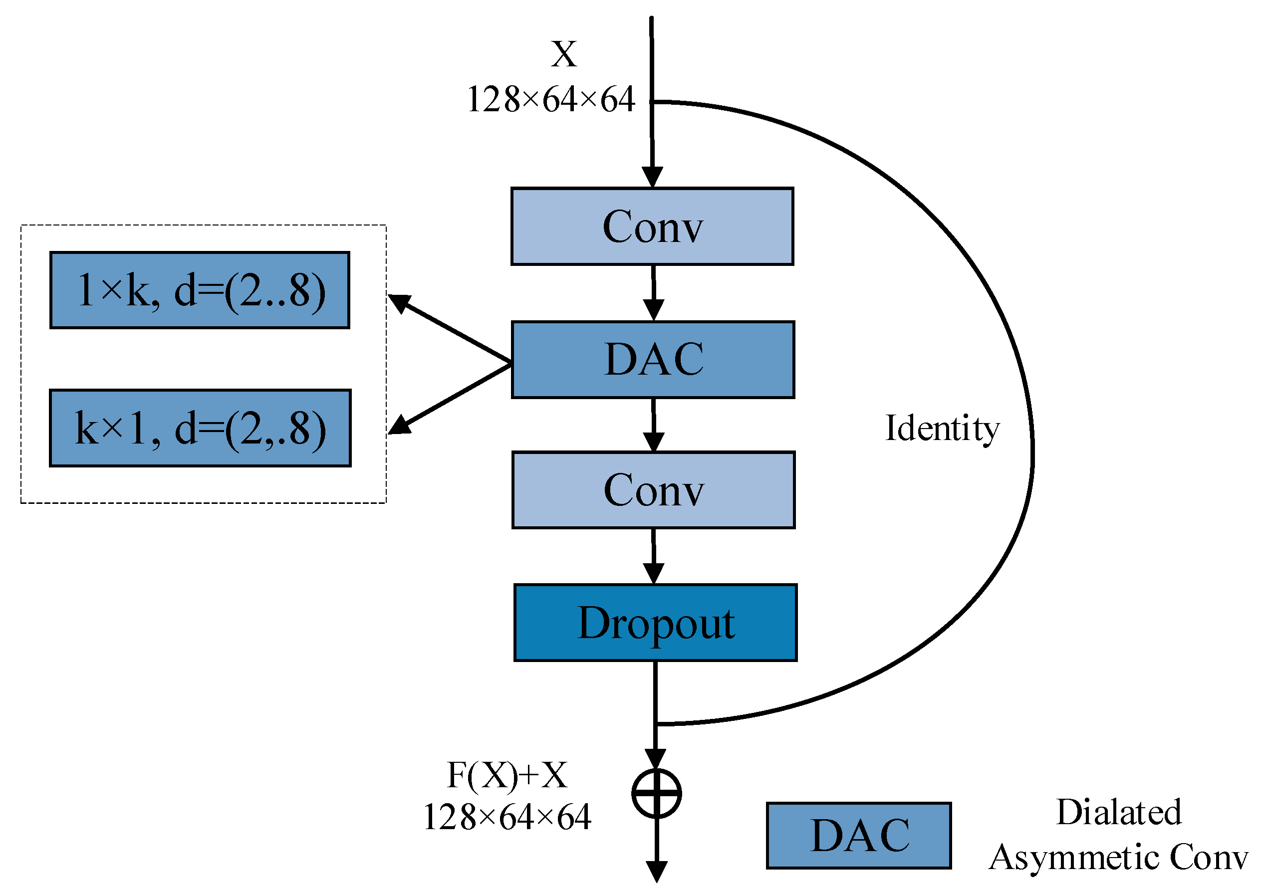
In the previous section, we pruned ENet and removed the third stage that duplicated the second stage, successfully lightweighting it. The ice-covered segmentation of transmission lines faces the challenge of distinguishing between the special shape structure and complex background of transmission lines, requiring a balance between context perception and detail preservation. Therefore, we restructured the bottleneck of ENet and proposed a DABM. By combining dilated convolution and asymmetric convolution, asymmetric convolution was used to improve the extraction of the morphological details of ice-covered transmission lines, and dilated convolution was used to expand the receptive field range of the model without increasing the number of parameters. Figure 1 presents a schematic diagram of the structure of the DABM.

Firstly, the image features are reduced in dimensionality through a 1 × 1 convolution block to reduce the computational complexity of the model. Then, the DAC convolution block is used to extract detailed information. The design of asymmetric convolution makes the model more friendly to slender objects such as transmission lines, and, by splitting the ordinary convolution, it further reduces the number of parameters in the convolution layer, which is conducive to deployment on edge terminals. Finally, the image dimension is restored to its original size through a 1 × 1 convolution block for subsequent calculations. The calculation formula for the DAC part is as follows:

$$X_{1\times k}\left(i,j,c\right)={\Sigma }_{t=0}^{k-1}X(i+p,j+t\times r+p,c)\times w_{1\times k}\left(t,c\right)$$

(1)

$$p={\displaystyle \frac{(k-1)\times r}{2}}$$

(2)

The input feature map is $X$, the spatial coordinates are $\left(i,j\right)$, the channel index is $c$, the dilation rate is $r$, and the convolution kernel size is $k$. $w_{1\times k}\left(t,c\right)$ is the weight of the $1\times k$ convolution kernel at position t and in channel c. $p$ is the padding value. First, a $1\times k$ dilated convolution is performed, and then a $k\times 1$ dilated convolution is performed on $X_{1\times k}$:

$$X_{dac}\left(i,j,c\right)={\Sigma }_{s=0}^{k-1}{X}_{1\times k}\left(i+s\times r+p,j+p,c\right)\times w_{k\times 1}\prime \left(s,c\right)$$

(3)

$w_{k\times 1}\prime (s,c)$ is the weight of the k × 1 convolution kernel at position $s$ and in channel $c$. We replace the last three bottlenecks in the first stage with the DABM. Through this operation, the underlying detailed information will be more fully excavated during feature extraction, laying the foundation for subsequent feature extraction. In addition, differentiated expansion rates of 2, 4, and 8 are designed in the three DABMs. By designing with different expansion rates, it is possible to finely capture the characteristics of ice-covered transmission lines at different scales. Convolution with small expansion rates has a strong ability to capture the detailed features of ice-covered transmission lines, while convolution with medium expansion rates has a moderate receptive field, which can capture both detailed information and local contextual information. Finally, the large expansion rate is used to obtain the overall characteristics of long-distance ice cover. In the second stage, we conduct re-planning by replacing bottlenecks 2.2, 2.4, 2.6, and 2.8 with DABMs.

We reconstruct the network model of ENet after pruning using the DABM, effectively improving the feature extraction ability of the model for ice-covered transmission line images. In the DABM, asymmetric convolution reduces the number of model parameters, while dilated convolution enhances the model’s perceptual ability without increasing the number of model parameters. Therefore, the reconstructed ENet does not significantly increase the number of model parameters.

3.4. Efficient Patial Conv Module (EPCM)

In the previous section, we replaced some of the convolutional blocks with DABMs, but there was still room for optimization in the remaining convolutional blocks. Therefore, in order to make the segmentation network more suitable for edge computing terminals, we introduced partial convolution (PConv) into the bottleneck, replacing the ordinary convolution in the bottleneck structure and reducing the number of model parameters and amount of computation. In addition, we designed an efficient partial convolution module based on PConv, introducing an adaptive filtering mechanism for selecting partial channels to further improve the accuracy of ice-covered segmentation.

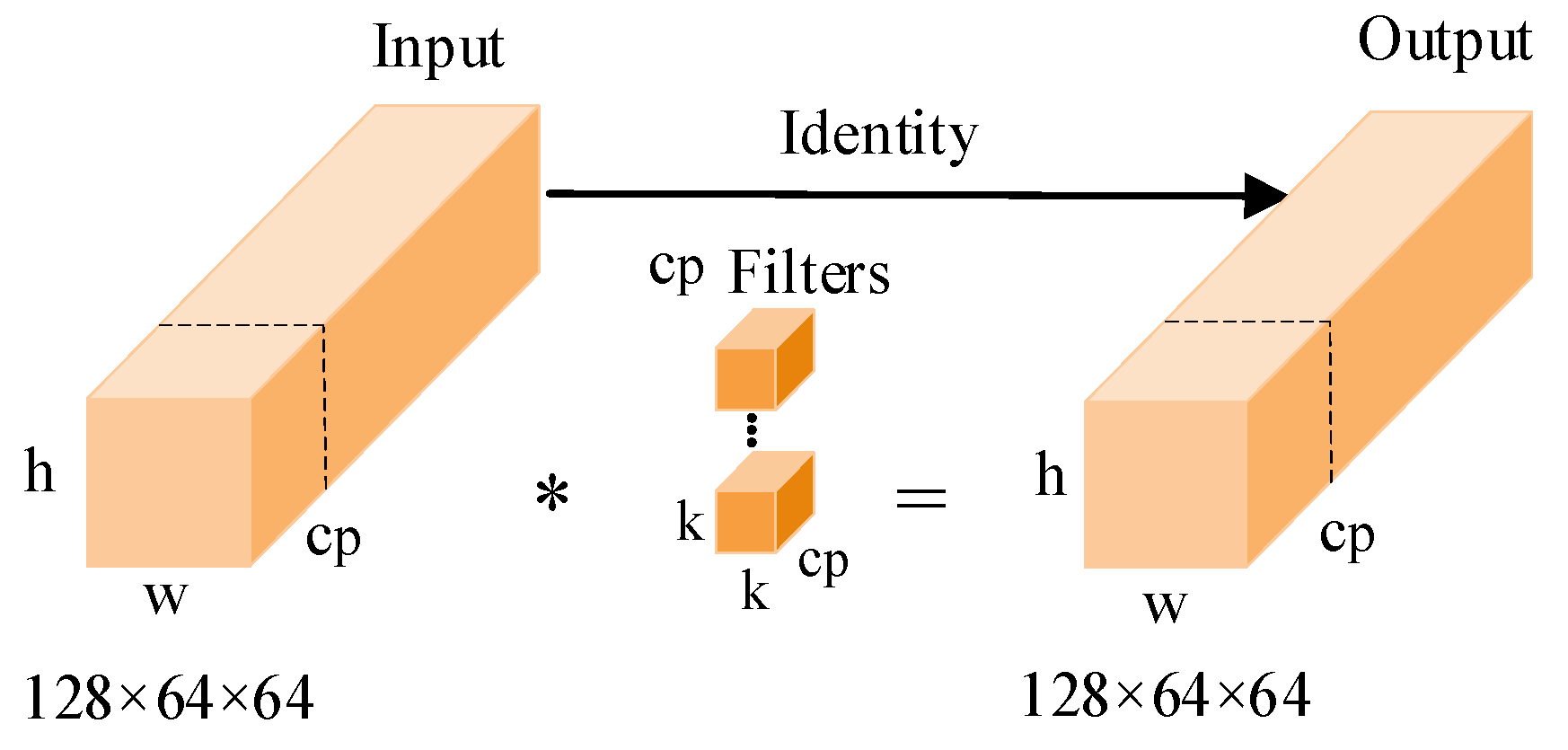
In convolution operations, different channels in the feature map have a high degree of similarity, and, inspired by this, partial convolution (PConv) was proposed. Partial convolution is an efficient convolution operator that partitions the channels of input features, only performing convolution calculations on some channels while keeping the remaining channels unchanged. This selective calculation can reduce computational redundancy in convolution calculations, improve computational efficiency, and extract image features more efficiently. A structural schematic of PConv is shown in Figure 2. The * in Figure 2 represents the convolution operation.

Usually, the convolutional channels involved in the calculation account for a quarter of the input channels. Partial convolution can reduce the FLOPS of ordinary convolution to one-sixteenth, effectively improving the performance of the model on edge devices. We apply partial convolutions to the bottleneck module of ENet, replacing ordinary convolutions with partial convolutions to improve the computational efficiency of the bottleneck module between the dimensionality reduction and enhancement of 1 × 1 convolutions.

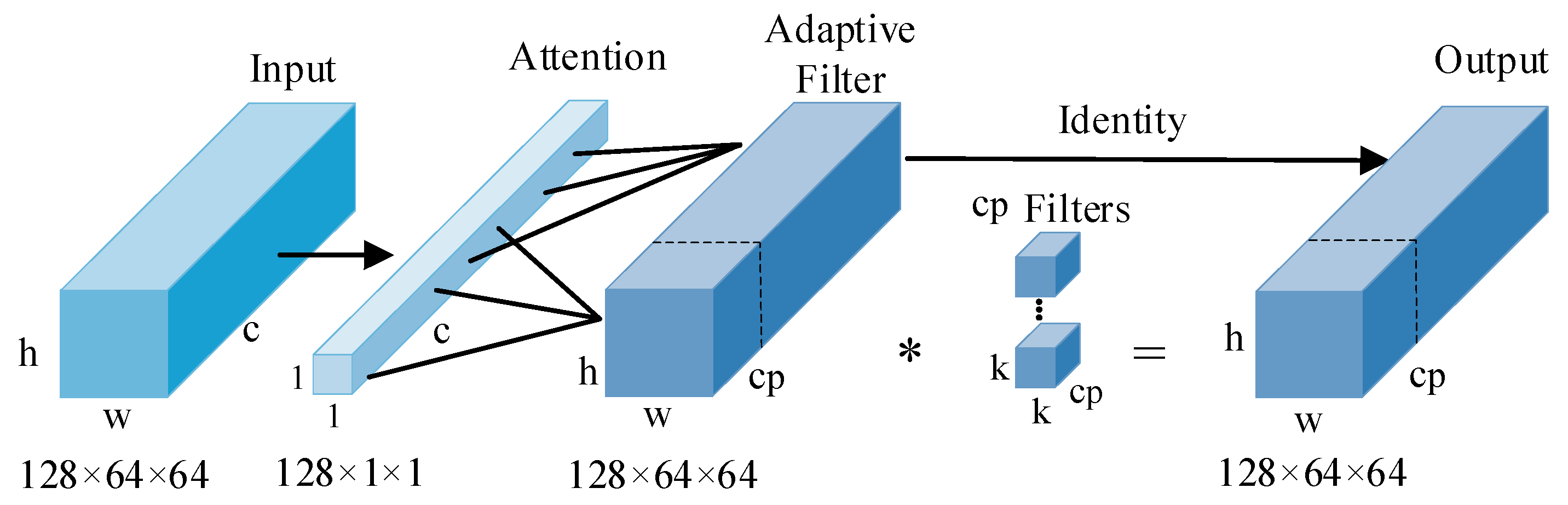
When PConv performs partial convolution channel partitioning, the selected channels are random, which may result in some unimportant channels also participating in the convolution operation, while channels that do not participate in the operation may contain features that are beneficial for the final segmentation. Therefore, achieving the effective filtering of some convolutional channels will be beneficial for the segmentation of ice-covered areas. Based on this, we propose an EPCM, which innovatively integrates partial convolutional (PConv) and the adaptive filtering mechanism. A schematic diagram of the EPCM structure is shown in Figure 3.

When image features are input, 1 × 1 convolutional blocks are still used to reduce the dimensionality in order to reduce the computational complexity of the feature extraction process. Then, an efficient attention ECA mechanism is introduced to automatically obtain the importance weight of each channel through the calculation of the ECA module. The ECA module is a lightweight channel attention mechanism that captures the dependencies between channels through one-dimensional convolution. Firstly, the input features are globally averaged pooled in the spatial dimension to obtain the pooled vectors of all channels. Then, one-dimensional convolution is used to process the pooled vectors, and, finally, the importance weights of each channel are obtained using the Sigmoid function. The calculation formula is as follows:

$$\alpha \left(c\right)=sigmoid\left({conv}_{1d}\right(F_{avg},W_{eca}\left)\right)$$

(4)

$F_{avg}$ is the feature vector after global average pooling, $W_{eca}$ is the weight of one-dimensional convolution, and the channel attention weight is obtained through the Sigmoid function. Based on the channel attention weights, the EPCM divides channels into important channels and unimportant channels. For important channels, convolution, normalization, and other operations are performed while keeping unimportant channels unchanged. Through this adaptive filtering mechanism, not only can unnecessary calculations be reduced and computational efficiency improved, but image features can also be effectively extracted, enhancing the model’s ability to extract key information. The calculation formula for partial convolution is as follows:

$$X_{pconv}\left(c\right)=\left\{\begin{array}{lll}Conv\left(X_1\left(c\right)\right)+b,& if \alpha \left(c\right)>\tau & \\ X_1\left(c\right), otherwise& & \end{array}\right.$$

(5)

Here, $\alpha \left(c\right)$ is the importance weight, and $\tau$ is the threshold. The EPCM can flexibly adjust the degree of control over channel screening by adjusting the threshold.

3.5. Calculation of Ice Thickness on Transmission Lines

After obtaining the ice-covered area from the ice image through EECNet, the total number of ice-covered pixels and background pixels is calculated by counting the ice-covered areas and non-ice-covered areas. The total sum of ice-covered pixels can represent the area of the ice-covered region, while the total sum of background pixels represents the area of the non-ice-covered region, which can be used to calculate the proportion of the ice-covered region in the entire image. Next, the proportion of the transmission line in the image without ice cover is calculated and combined with the known radius of the transmission line to determine the ice thickness on the transmission line. The specific calculation formula is as follows:

$${\displaystyle \frac{P_{line}}{P_{ice}}}={\displaystyle \frac{r}{r+d}}$$

(6)

The ice thickness $d$ is obtained by solving the following:

$$d=r( {\displaystyle \frac{P_{ice}}{P_{line}}}-1)$$

(7)

Here, r is the radius of the transmission line, and $P_{ice}$ is the proportion of the ice-covered area in the image, whose calculation formula is as follows:

$$P_{ice}=Count\left(N_{ice}\right)$$

(8)

$N_{ice}$ is the total number of pixels in the image of the ice-covered area, and $P_{line}$ is the proportion of the transmission line in the image without ice cover, whose calculation formula is as follows:

$$P_{line}=Count\left(N_{line}\right)$$

(9)

$N_{line}$ is the total number of pixels in the image for areas without ice cover.

3.6. EECNet

We propose EECNet by implementing a series of optimization and improvement measures on ENet. Firstly, the ENet model is pruned to remove the repetitive third stage, reducing the model’s parameter count and computational complexity. Secondly, the bottleneck of the second stage is reconstructed, and a DABM is proposed, which enhance the ability to extract the slender-shaped features of transmission lines and improve the model’s perception of image features at different scales. Finally, an EPCM is designed, innovatively combining partial convolution with adaptive filtering to enhance the model’s ability to extract key information. Figure 4 presents a schematic diagram of EECNet.

The entire model is divided into two parts: an encoder and a decoder. The encoder includes the initial stage, the first stage, and the second stage, while the decoder includes the third stage and the fourth stage. The encoder part consists of the DABM, EPCM, and downsampling module, while the decoder consists of the bottleneck module and upsampling module.

4. Experimental Results and Analysis

4.1. Experimental Dataset and Environment

Since there is currently no publicly available dataset for ice-covered transmission lines, we constructed a real transmission line in winter to capture images of ice-covered transmission lines. The dataset used in this experiment consists of two parts, most of which consists of real ice images captured outdoors when cables were successfully covered with ice and snow during winter snowfall. The other part consists of existing images of ice-covered transmission lines that were collected from the internet, filtered, downloaded, and organized. Finally, the images were organized and annotated, and data augmentation techniques such as affine transformation were used to obtain 1469 experimental images. All experimental samples were randomly divided into a training set and a testing set, with a ratio of 8:2. All experiments in this section were conducted in the same environment, and the experimental environment and hyperparameters are detailed in

Table 2. Experimental environment and hyperparameters.

Parameter	Parameter Settings
Operating System	Ubuntu20.04
Python Version	3.7.16
Deep Learning Framework	Pytorch1.13.1
GPU	RTX4090
Batch Size	36
Optimizer	SGD
Learning Rate	0.0001
Number of Iterations	1800
Random Invert	0.5
Random Rotation	−15–15°
Brightness	0.5–1.5

.

4.2. Evaluation

The metrics commonly used to evaluate model performance in image segmentation are the mIoU and F1-Score. The mIoU is the average ratio of the intersection and union between the predicted area and the real segmentation area, reflecting the overall overlap between the predicted area and the real area. The calculation formula is as follows:

$$mIoU={\displaystyle \frac{1}{N}}\Sigma {\displaystyle \frac{TP}{TP+FP+FN}}$$

(10)

The TP (True Positive) is the number of pixels correctly predicted as positive, the FP (False Positive) is the number of pixels incorrectly predicted as positive, and the FN (False Negative) is the number of pixels incorrectly predicted as negative. N is the number of predicted categories. The higher the value of mIoU, the more accurate the segmentation. A value of 1 indicates that the predicted result is consistent with the true label, and a value of 0 indicates that there is no overlap between the two. The F1-Score is the harmonic mean of precision and recall, reflecting the prediction accuracy of positive samples. Its calculation formula is as follows:

$$F1={\displaystyle \frac{P\times R\times 2}{P+R}}$$

(11)

where $P$ represents precision, and $R$ represents recall. Consistent with the mIoU, its value range is 0–1, with higher values indicating more accurate model predictions. In this part of the experiment, we selected these two parameters to evaluate the effectiveness of EECNet.

4.3. Ablation Experiment

In order to verify the effectiveness of the EECNet improvement module, in this section, we designed ablation experiments to evaluate the effectiveness of each module, with a total of four sets of experiments designed. Experiment 1 involved the original ENet, Experiment 2 involved the pruned ENet, Experiment 3 added the DABM to the pruned network, and Experiment 4 involved EECNet, with the EPCM integrated into the network model. The experiments were conducted on the ice-covered dataset of transmission lines, and the results are shown in

Table 3. Results of model ablation experiment.

Experiment	mIoU/%	F1-Score/%	Parameter /M	GFLOPS
Exp 1	91.8	95.7	0.36	2.35
Exp 2	91.1	95.3	0.21	1.73
Exp 3	92.0	95.8	0.21	1.76
EECNet	92.7	96.2	0.21	1.67

.

In Table 3, it can be seen that, compared with Experiment 1, Experiment 2 significantly reduced the number of parameters and GFLOPS, and the adverse effect of model lightweighting was a decrease in detection accuracy. Experiment 3 reconstructed the pruned model by integrating dilated convolution and asymmetric convolution, resulting in a 0.9% increase in the mIoU and a 0.5% increase in the F1-Score. The model parameters and computational complexity did not increase. Finally, the EPCM was added to the reconstructed model, and, with its adaptive selection convolution mechanism, the mIoU and F1-Score were further improved, reaching 92.7% and 96.2%, respectively. It is worth noting that, due to the addition of some convolutions, the computational complexity of the model also decreased. Table 1 clearly demonstrates the improvement of each improvement module on the final segmentation accuracy, and the experimental results also prove that EECNet effectively enhances the network’s feature extraction ability while lightweighting ENet. We conducted three independent experiments on EECNet and verified the stability of the model by setting different random seeds.

Table 4. Independent experimental results.

Experiment	mIoU/%	F1-Score/%
Exp 1	92.8	96.3
Exp 2	92.6	96.1
Exp 3	93.0	96.4
Mean value	92.8	96.2

shows the results of the Independent experiment. The statistical significance analysis is shown below.

By calculation, the mIoU mean $\overline{x}$ is 92.8%, the sample standard deviation $s$ is 0.2%, the sample size $n$ is 3, and the 95% confidence level corresponds to a value of 0.05 for $\alpha$. According to the t-distribution table, $t_{\alpha /2,df}$ = 4.303. The confidence interval is calculated according to the following formula:

$$\overline{x}\pm t_{\alpha /2,df}\times {\displaystyle \frac{s}{\sqrt{n}}}$$

(12)

The calculated confidence intervals are [92.3%, 93.3%], covering 92.7% of the reported data in the paper. Similarly, the F1-Score mean is 96.2%, and the calculated sample standard deviation s is 0.17%. After applying the formula, the 95% confidence interval is found to be approximately [95.8%, 96.6%], including the 96.2% reported in this paper. Through experimental verification, it is found that the model is controllable under the influence of random seeds, and the results are statistically significant.

4.4. Asymmetric Convolutional Kernel Experiment

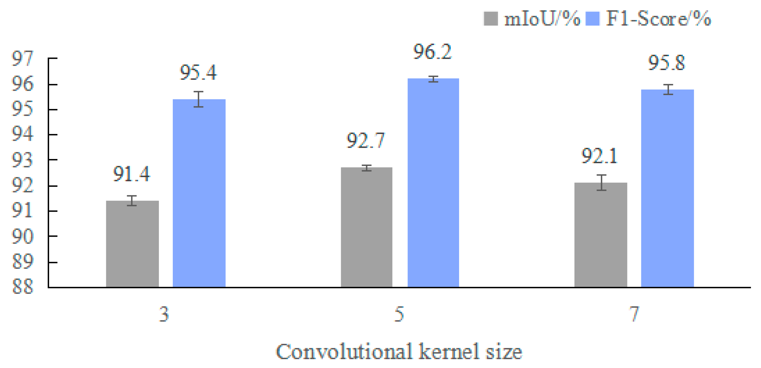
The asymmetric convolution in the DABM enhances the ability to extract ice features on transmission lines, where different convolution kernels correspond to different receptive field ranges. Therefore, an experimental analysis is conducted on the size of the convolution kernels to study the optimal parameters for asymmetric convolution. The experimental results are shown in Figure 5.

In Figure 5, it can be seen that, when the convolution kernel is set to 5, the mIoU and F1-Score of the model are the highest. When the convolution kernel is 3, the receptive field of the model is small and can only extract local features. When the size of the convolution kernel is 7, the range of feature extraction by the model becomes larger, ignoring detailed information. Therefore, setting the convolution kernel of asymmetric convolution to 5 is the most suitable, which can balance local detail information and obtain a larger receptive field range.

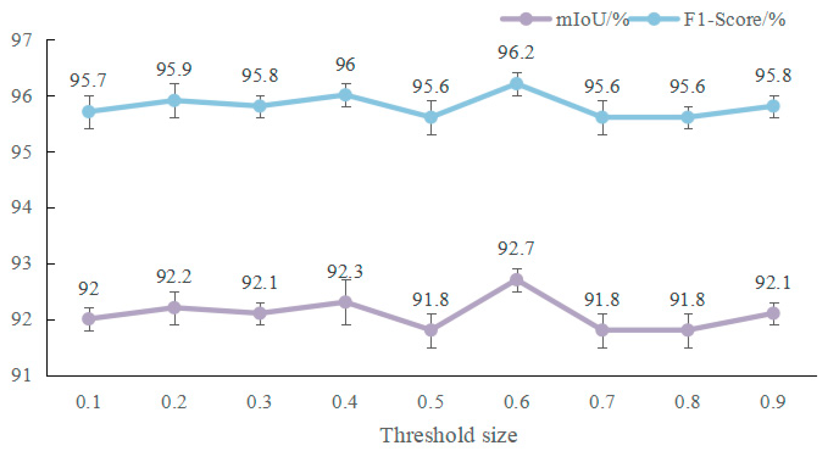
4.5. Adaptive Threshold Experiment

In the EPCM, we introduce an adaptive channel selection mechanism that divides the channels of image features into important and non-important channels, with the ratio of division determined by an adaptive threshold. Therefore, in this section, we conduct experiments on adaptive thresholding to find the optimal partition point. The experimental results are shown in Figure 6.

From the experimental results, it can be seen that, when the adaptive threshold is set to 0.6, the segmentation effect of EECNet is the best. At this time, the proportion of important channels to the entire channel is 0.6, indicating that the EPCM can filter out most of the information that is beneficial for the final segmentation. When the threshold is set too low, the proportion of features filtered by the EPCM is insufficient, so most channels do not participate in the operation. When the threshold is set too high, some non-important channels are mixed in, which has a negative impact on the final segmentation. Therefore, in subsequent experiments, we set all adaptive thresholds to 0.6.

4.6. Comparison Experiment with Other Algorithms

In order to compare the EECNet method with other segmentation algorithms, we conducted eight sets of comparative experiments involving ENet, DABNet, UNet, Segformer, FastSegFormer, DeepLabV3-Mobile [40], HRNet-W18s [41], and BiseNet. This included lightweight networks, segmentation networks with convolutional neural networks as the backbone, and Segformer using the Transformer architecture. The experimental results are shown in

Table 5. Comparison of experimental results with those of other algorithms.

Model	mIoU/%	F1-Score/%	Parameter /M	GFLOPS	FPS
ENet	91.8	95.7	0.36	2.35	11
DABNet	93.0	96.3	0.75	5.29	9
UNet	93.4	96.5	1.08	10.22	4
Segformer	86.9	92.8	7.71	13.10	1
FastSegFormer	92.7	96.1	14.87	2.70	1
DeepLabV3-Mobile	92.1	95.8	26.43	5.81	2
BiseNet	92.9	96.3	12.8	13.05	8
HRNet-W18s	93.5	96.6	4.0	10.2	2
EECNet	92.7	96.2	0.21	1.67	14

.

From the analysis in the table above, it can be seen that EECNet has the lowest parameter count and computational complexity. In terms of segmentation performance, DABNet, UNet, and BiseNet perform better than EECNet, but their real-time detection performance is not as good as that of EECNet, and the detection accuracy is not significantly different. Segformer is the only Transformer architecture model, but, due to its unique architecture, it does not show good performance in the task of ice-covered transmission line segmentation, and its model parameters do not provide advantages. Therefore, EECNet reduces the number of model parameters and computation while maintaining detection accuracy, improving detection speed. Figure 7 shows the detection comparison of the different algorithms, demonstrating the effectiveness of ice-covered area segmentation under different conditions. In Figure 7, it can be seen that, under a simple background, all algorithms can identify the ice-covered area. In complex backgrounds, ENet exhibits phenomena of missed and false detections. Among them, UNet performs the best, but its parameter count is much larger than that of EECNet. Segformer performs poorly and has the highest number of missed areas compared to the other algorithms in complex backgrounds, indicating that this type of algorithm is not suitable for the task in this paper. Our proposed EECNet can accurately recognize ice-covered images in both single scenes and complex backgrounds.

4.7. Ice Thickness Experiment on Transmission Lines

After obtaining the ice-covered segmentation image, the calculation of ice thickness can be carried out. According to the analysis of the ice-covered image, the entire image is divided into two parts. The white area, with a pixel value of 255, is the foreground part, and the black area, with a pixel value of 0, is the background part. By using the pre-measured actual diameter of the ice-free transmission line and the difference in pixel area between the images before and after the development of ice cover, the ice thickness can be derived. By quantifying the correspondence between image pixels and actual physical quantities, an accurate measurement of ice thickness can be achieved. When collecting ice-covered images, we use a vernier caliper to synchronously record the actual ice thickness, and we compare the predicted ice thickness with the collected actual ice thickness on the transmission line. The experimental results are shown in

Table 6. Ice thickness test for transmission lines.

Actual Thickness/mm	Test Method	Predicted Thickness/mm	Error/%
4.8	EECNet	4.7	2.1
	ENet	4.4	8.3
7.6	EECNet	7.8	2.6
	ENet	7.3	3.9
11.5	EECNet	12.0	3.4
	ENet	12.1	5.2

.

In Table 6, it can be seen that, compared with ENet, EECNet has a thickness recognition error of less than 3.4%, and the predicted value does not exceed the true value by 1mm. The experimental results demonstrate that the method proposed in this paper can accurately identify the ice thickness on transmission lines.

4.8. Edge Computing Terminal Deployment

Deploying EECNet on an edge computing terminal for transmission line ice thickness detection can improve the real-time performance of detection. Therefore, in this section, we conduct experiments on the detection speed of EECNet and ENet on OrangePi 5 Pro, Shenzhen Xunlong Software Co., Ltd., Shenzhen, China. The edge computing terminal uses an rk3588s chip and has 6Tops of NPU computing power, which can accelerate the reasoning of the deep learning model. The final experimental results are shown in

Table 7. Results of model deployment experiment.

Model	Time/ms	FPS
ENet	86	11
EECNet	69	14
ENet (quantization)	53	19
EECNet (quantization)	41	24

.

It can be seen in Table 7 that EECNet can achieve a 14FPS reasoning speed on the edge computing terminal, which is 3FPS higher than that of ENet, and the detection speed is 17ms lower. After quantifying EECNet, the detection speed can be optimized to 41ms, and the frame rate can be improved to 24FPS. The experimental results show that EECNet significantly improves the detection speed of ice thickness compared to ENet.

5. Conclusions

For the recognition of ice thickness on transmission lines, this paper proposes a network called EECNet, which is suitable for edge computing. Due to its lightweight and innovative design, the detection accuracy of the model did not decrease when reducing the number of model parameters. Firstly, ENet was pruned to remove redundant parts, significantly reducing the number of model parameters. Secondly, by restructuring the bottleneck and redesigning the DABM, the model’s ability to extract features from ice-covered areas improved. Finally, an EPCM was proposed, which enhances the ability to focus on important channels while reducing model computation by introducing an adaptive filtering mechanism. Experiments were conducted on an ice-covered transmission line dataset, and EECNet achieved an mIoU value of 92.7% and an F1-Score of 96.2%. Compared to ENet, the model parameters decreased by 41.7%, and the computational complexity decreased by 29%. The recognition speed on edge computing terminals increased by 3FPS. The experimental results show that EECNet can effectively improve the detection speed of edge devices and accurately identify ice thickness.

In the future, we will continue to research algorithms for identifying ice thickness on transmission lines and continuously improve our detection capabilities on edge devices. In addition, the combination of image information and meteorological information will be considered to enhance recognition accuracy through richer information sources.