Data-Driven Fault Detection for HVAC Control Systems in Pharmaceutical Manufacturing Workshops

Abstract

Large-scale heating, ventilation, and air conditioning (HVAC) control systems in pharmaceutical manufacturing are characterized by complex operational parameters, delayed and often challenging fault detection, and stringent regulatory compliance requirements. To address these issues, this study presents an innovative data-driven fault detection framework that integrates Principal Component Analysis (PCA) with Nonlinear State Estimation Technology (NSET), specifically tailored for highly regulated pharmaceutical production environments. A dataset comprising 13,198 operational records was collected from the SCADA system of a pharmaceutical facility in Zhejiang, China. The data underwent preprocessing and key parameter extraction, after which a nonlinear state estimation predictive model was constructed, with PCA applied for dimensionality reduction and sensitivity enhancement. Fault detection was performed by monitoring deviations in the mixing room temperature, identifying faults when the residuals between observed and predicted values exceeded a statistically determined threshold (mean ± three standard deviations), in accordance with the Laida criterion. The framework’s effectiveness was validated through comparative analysis before and after documented fault events, including temperature sensor drift and abnormal equipment operation. Experimental results demonstrate that the proposed PCA-NSET model enables timely and accurate detection of both gradual and abrupt faults, facilitating early intervention and reducing potential production downtime. Notably, this framework outperforms traditional fault detection methods by providing higher sensitivity and specificity, while also supporting continuous quality assurance and regulatory compliance in pharmaceutical HVAC applications. The findings underscore the practical value and novelty of the integrated PCA-NSET approach for robust, real-time fault detection in mission-critical industrial environments.

1. Introduction and Literature Review

1.1. Introduction

In pharmaceutical manufacturing, the environmental conditions of production workshops—including temperature, humidity, cleanliness, and pressure differentials—directly affect the quality and safety of pharmaceutical products [1,2]. Different types of pharmaceuticals impose distinct requirements on these environmental parameters. To ensure that production environments meet stringent regulatory standards, it is essential to employ reliable HVAC (heating, ventilation, and air conditioning) control systems to regulate the operation of all critical equipment [3]. Consequently, the adoption of effective monitoring and fault detection techniques is of great significance for maintaining high product quality and production yield.

Modern HVAC systems in pharmaceutical workshops typically regulate critical air-handling components—including chilled water valves, hot water valves, and humidification valves—to ensure environmental parameters such as temperature, humidity, and pressure remain within strictly controlled setpoints required by industry regulations [4]. Over the past decade, the widespread deployment of SCADA (Supervisory Control and Data Acquisition) platforms has enabled real-time, high-resolution data acquisition, providing a rich basis for advanced modeling and analysis in industrial environments [5]. By effectively utilizing this data, data-driven models can be constructed to predict system behavior under normal operating conditions, allowing for the detection of abnormal deviations through residual analysis [6].

Despite the proliferation of physical- and empirical-model-based fault detection methods, their practical application in complex, dynamic industrial HVAC systems remains limited by requirements for expert knowledge and difficulties in adapting to evolving operational modes [7,8]. For example, model-based approaches often rely on detailed physical modeling and accurate parameter identification, which are resource-intensive and may not generalize well to varying system configurations. Rule-based and threshold-based methods, though simple to implement, typically struggle with noisy data and are prone to false alarms or missed detections in dynamic environments. Data-driven approaches such as artificial neural networks and support vector machines have also been investigated; however, these methods frequently suffer from interpretability issues and require large labeled datasets for effective training. Common HVAC faults—such as sensor drift, actuator sticking or failure, fan or compressor degradation, valve misalignment, or filter clogging—often manifest gradually and may go unnoticed during routine operations. Early detection of such faults is critical in pharmaceutical manufacturing, where environmental control is directly linked to product stability, sterility, and overall quality assurance [9]. Proactive fault detection not only minimizes unplanned downtime and reduces maintenance costs but also enhances system reliability and regulatory compliance, which are essential in Good Manufacturing Practice (GMP)-regulated environments [10].

Recent studies have shown that data-driven approaches, such as those based on dimensionality reduction and nonlinear modeling, offer promising advantages in capturing system variability and enabling robust early fault detection in HVAC systems [11]. However, there is a notable lack of research specifically targeting the unique operational constraints and regulatory requirements of pharmaceutical manufacturing, especially in the context of complex mode-switching and dynamic behavior.

To address these challenges, this work proposes an integrated approach combining PCA with NSET [12]. The main idea is to utilize PCA for data cleaning and dimensionality reduction of SCADA-acquired datasets, thereby constructing a temperature prediction model for the HVAC system under normal operation [13]. PCA helps filter out noise and redundant variables, enhancing the subsequent nonlinear modeling process. This enables real-time and accurate fault detection, facilitating the timely identification of potential failures and the implementation of preventive maintenance strategies to ensure the reliable and safe operation of the system. Compared to existing model-based, rule-based, and black-box machine learning approaches, the proposed PCA-NSET framework offers a balance of interpretability, scalability, and adaptability to complex industrial datasets, making it particularly suited for regulated pharmaceutical manufacturing. It is hypothesized that this PCA-NSET framework can overcome key limitations of existing methods—including limited interpretability, scalability, and adaptability to complex industrial data—thus providing a robust solution tailored to the stringent and evolving operational requirements of pharmaceutical manufacturing workshops.

1.2. Literature Review

In recent years, significant progress has been made in applying advanced data-driven techniques to HVAC fault detection in pharmaceutical and cleanroom environments. For example, deep learning models and ensemble learning strategies have achieved notable success in detecting sensor failures, system anomalies, and subtle degradations [14,15]. Research has also explored the integration of domain knowledge and explainable AI to improve the interpretability and robustness of fault detection frameworks [16,17]. However, these methods often suffer from limited interpretability and require large, labeled datasets for effective training, which may not always be feasible in pharmaceutical applications. Despite these advances, the majority of recent studies have focused on large-scale commercial buildings or general industrial settings, and there is a relative lack of high-quality research specifically targeting pharmaceutical manufacturing environments, where the regulatory and operational constraints are especially stringent.

Artificial neural networks, particularly those employing backpropagation algorithms, have been widely applied in the fault detection and diagnosis of HVAC systems and related equipment. Some studies have integrated backpropagation neural networks with decision tree methods to enhance the detection and classification of both known and unknown faults [18]. The introduction of algorithms such as Round Robin Dithering (RDP) has further simplified neural network models for fault detection, improving diagnostic efficiency without sacrificing accuracy [19]. While neural networks possess powerful learning capabilities [20], their diagnostic performance heavily depends on the quality and quantity of training data, and the resulting models often lack interpretability and extensibility, limiting their practical application. In contrast, the integration of PCA and NSET offers a more transparent, interpretable framework, which is particularly beneficial in pharmaceutical contexts where explainability is required by regulators.

PCA is a widely used linear dimensionality reduction technique that can effectively capture dominant patterns in multivariate process data. However, its capacity to represent nonlinear relationships and subtle anomalies is inherently limited [21]. NSET is a data-driven, nonparametric, and nonlinear empirical modeling method. It has been successfully applied to early fault warning in wind turbine generators [22], and further improvements have been achieved by integrating additional fault detection algorithms to enhance prediction accuracy. However, the effectiveness of NSET relies on the selection of a representative process memory matrix constructed from historical data. This approach has notable limitations, including (i) expert-selected samples may lack representativeness, and (ii) selecting too many historical samples can result in an excessively large memory matrix [23]. Moreover, NSET models are sensitive to parameter settings and may struggle with generalizability under diverse or dynamic working conditions. In summary, although recent years have witnessed ongoing advancements in fault detection methods for pharmaceutical HVAC systems, there remains a lack of systematic benchmarking and critical comparison under strict regulatory constraints. Therefore, further efforts are needed to evaluate the suitability and performance of various advanced algorithms in this unique industrial context. The proposed PCA-NSET approach addresses these limitations by using PCA for effective data cleaning and dimensionality reduction prior to NSET modeling, thereby improving model robustness, reducing computational complexity, and enhancing fault sensitivity even under stringent regulatory constraints.

2. Materials and Methods

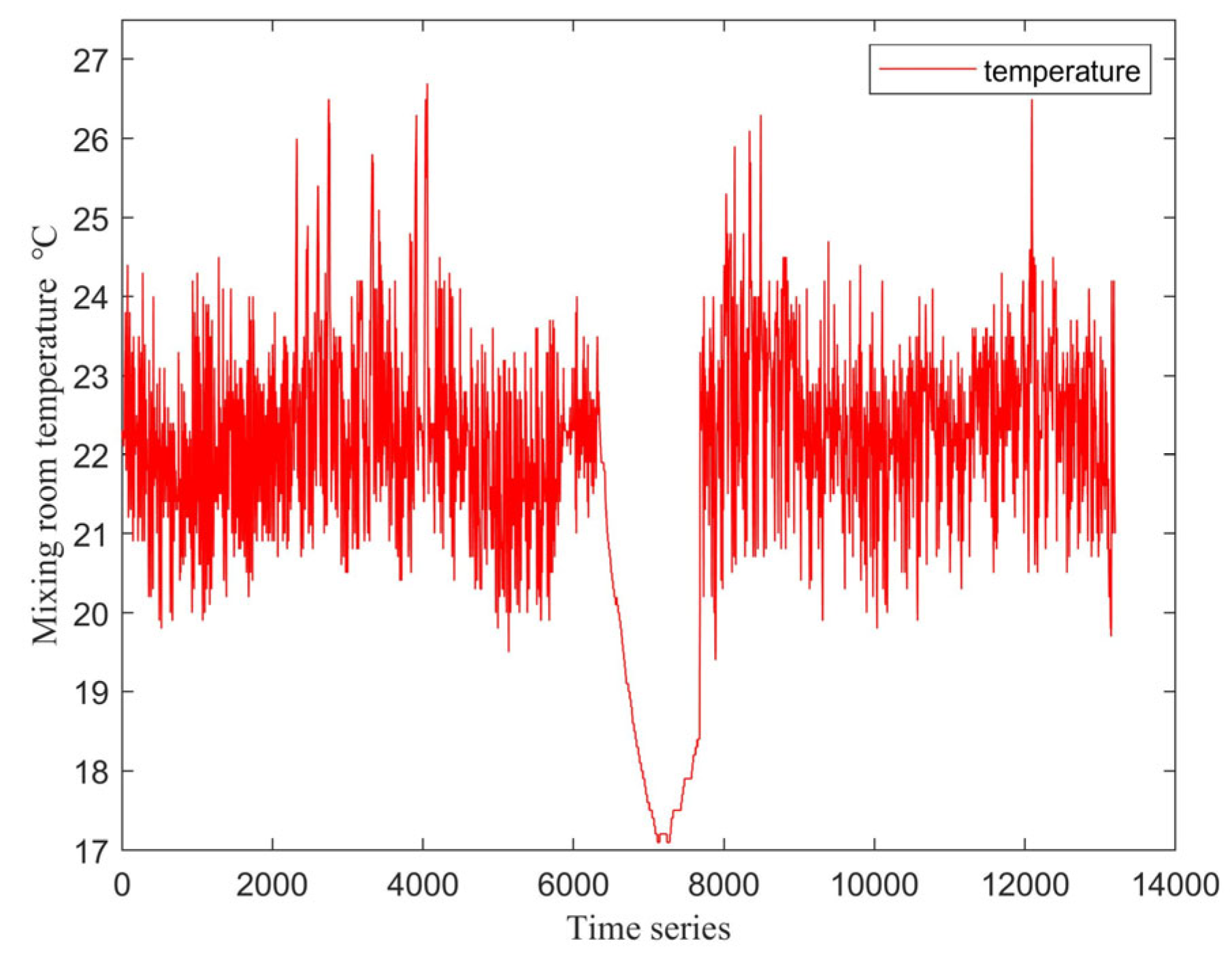
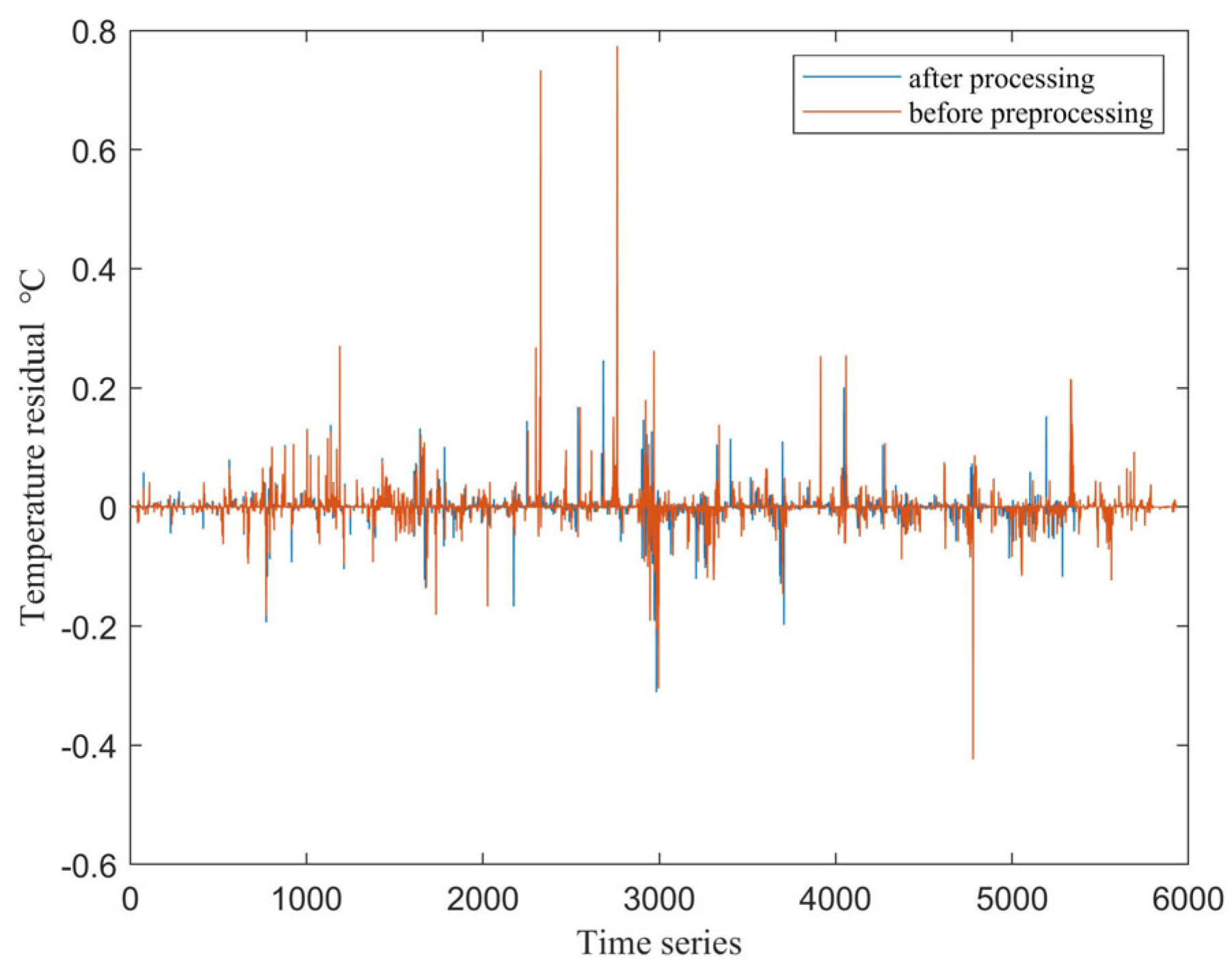
2.1. Data Preprocessing

When the number of measurements is sufficiently large, it can be assumed that the sample data follow a normal distribution [24]. Assuming the data contain only random errors, the standard deviation of the dataset can be calculated to define a confidence interval. Any measurement error that falls outside this interval is considered a gross error, which can be identified as an outlier or abnormal data point [25].

Let a set of measurements be denoted as $x_i\left(i=1,2,\cdots ,n\right)$, The mean $\overline{x}$ and deviation $v_i=x_i-\overline{x}$ of the dataset are calculated. If, for a particular data point $x_k$, the deviation $v_k$$\left(1\le k\le n\right)$ satisfies the following condition:

$$\left|v_k\right|=\left|x_k-\overline{x}\right|>3\sigma$$

(1)

then the data point $x_k$ is considered to be an outlier.

Raw data must be normalized before further processing to eliminate the influence of different units and scales [26]. Z-score normalization is a commonly used method for standardizing data. This approach standardizes the original data based on its mean and standard deviation, which alters the scale of the data but does not change the type of its distribution [16]. Z-score normalization is particularly suitable for situations where the maximum and minimum values of the dataset are unknown.

$$x_n{\left(m\right)}^{\prime }={\displaystyle \frac{x_n\left(m\right)-\mu }{\sigma }}$$

(2)

In Equation (2), $x_n{\left(m\right)}^{\prime }$ denotes the standardized data, $\mu$ represents the mean of the sample data, and $\sigma$ is the standard deviation of the sample data. After standardization, the processed data follow a distribution with a mean of 0 and a standard deviation of 1.

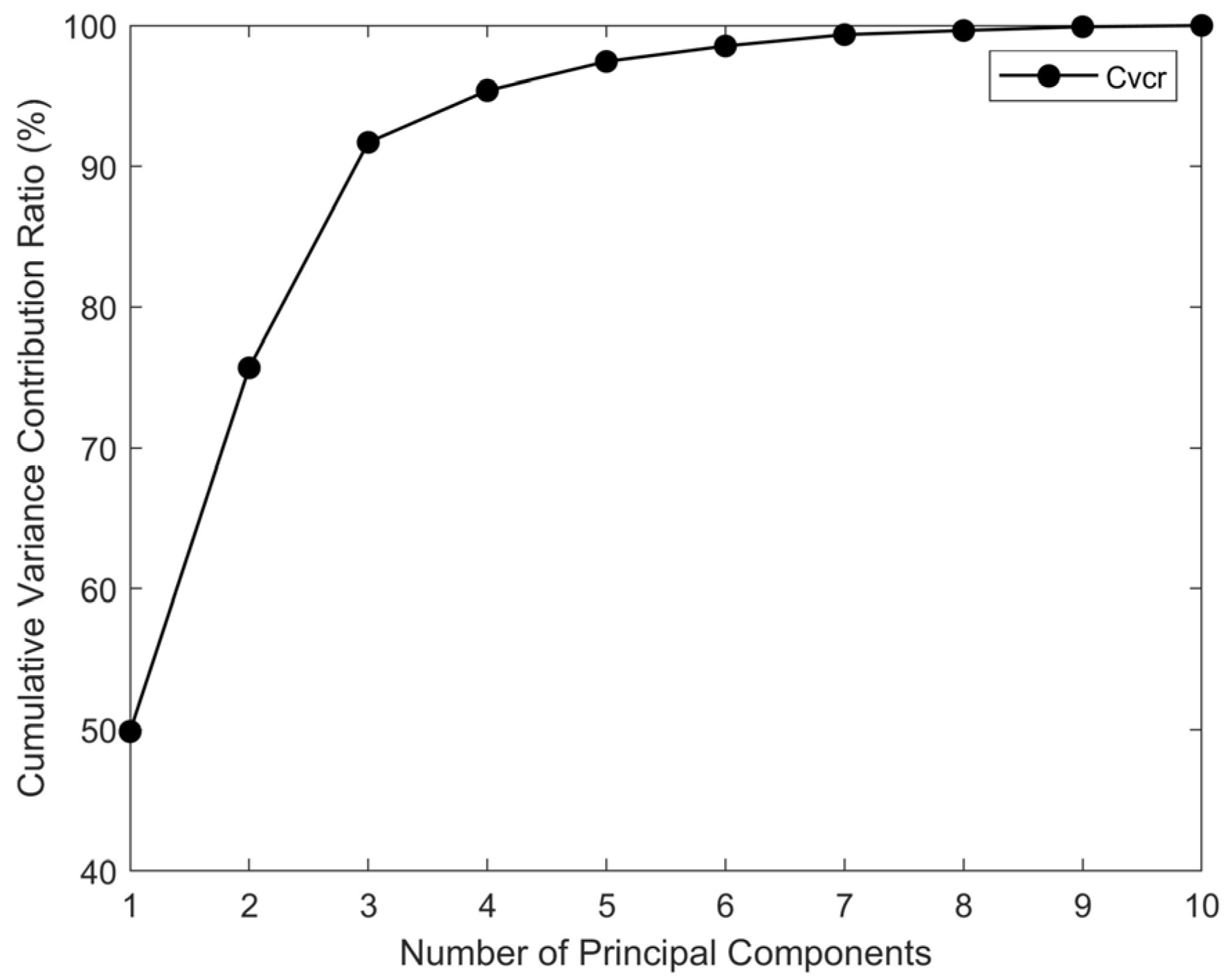
2.2. Feature Selection and Principal Component Analysis

The object of this study is the HVAC system of a pharmaceutical manufacturing facility located in Zhejiang Province, China. This system controls three separate rooms: the weighing room (w-room) for measuring raw materials, the preprocessing room (p-room) for preliminary handling of ingredients, and the mixing room (m-room) for final product manufacturing. To develop the NSET model for temperature prediction in the mixing room, it is necessary to identify the parameters in the SCADA system that are most closely related to the mixing room temperature [27,28]. The parameters recorded by the SCADA system, along with their Pearson correlation coefficients with the mixing room temperature and their respective operating ranges, are summarized in

Table 1. Operating parameter ranges and correlation analysis with mixing room temperature.

Parameter	Operating Range	Pearson Correlation Coefficient
Supply air duct humidity	[13.4, 73.2]	−0.280
Supply air duct flow rate	[4912, 11,687]	−0.167
Fan frequency	[34.8, 50]	−0.181
Workshop air flow rate	[57.5, 22,268]	−0.146
Mixing room temperature	[18.8, 26.7]	1
Mixing room humidity	[21, 68.1]	−0.191
Weighing room temperature	[18.8, 25.7]	0.831
Weighing room humidity	[22.1, 71.9]	−0.108
Preprocessing room temperature	[19, 26.4]	0.900
Preprocessing room humidity	[21.8, 70.6]	−0.280

All temperature values are in °C, humidity in %RH, flow rate in m³/h, frequency in Hz.

.

As shown in Table 1, the mixing room temperature exhibits a strong positive correlation with both the weighing room temperature and the preprocessing room temperature. This is primarily because all three rooms are regulated by the same HVAC system. However, it should be noted that the Pearson correlation coefficient has certain limitations. It is only suitable for describing linear relationships, is sensitive to outliers, and does not provide information about causal relationships [29]. Therefore, it is necessary to combine other methods for more robust and comprehensive variable selection in the modeling process.

PCA is a widely used dimensionality reduction algorithm [30]. The fundamental idea of PCA is to transform a set of correlated variables into a smaller number of uncorrelated composite variables, known as principal components, through linear combination. These principal components are designed to capture as much of the useful information from the original data as possible [31]. The specific steps for determining the principal components are as follows:

Suppose there are $n$ observed variables, denoted as $X_i=\left(x_{1i},x_{2i},\cdots ,x_{Ni}\right)$, $i=1,2,\cdots ,n$. Let the correlation coefficient between variables $X_s$ and $X_t$ $\left(s,t=1,2,\cdots ,n\right)$ be $r_{st}$. The principal steps for performing PCA are as follows:

• Data preprocessing. Prepare the raw data for analysis, typically involving normalization or standardization.
• Calculation of correlation coefficients. Compute the pairwise correlation coefficients among all variables to obtain the correlation coefficient matrix $R=\left(r_{st}\right),s,t=1,2,\cdots ,n$.
• Eigenvalue and eigenvector computation. Calculate the eigenvalues ${\lambda }_i$ and corresponding eigenvectors $e_i=\left(e_{i1},e_{i2},\cdots ,e_{ip}\right)$ of the correlation coefficient matrix $R$. The eigenvectors represent the directions of the principal components.
• Calculation of variance contribution rates. Determine the variance contribution rate $Vcr$ of each principal component, as well as the cumulative variance contribution rate $Cvcr$ of the first $l$ principal components.

  $$Vcr={\displaystyle \frac{{\lambda }_i}{{\displaystyle \sum _{i=1}^n{\lambda }_i}}},Cvcr={\displaystyle \frac{{\displaystyle \sum _{i=1}^l{\lambda }_i}}{{\displaystyle \sum _{i=1}^n{\lambda }_i}}}$$

  (3)

Principal Component Analysis was performed on the parameters recorded by the SCADA system using Equation (3). The contribution rates and cumulative contribution rates of all principal component vectors were calculated and then ranked in descending order of their contribution rates, as illustrated in Figure 1.

The variance contribution rates and cumulative variance contribution rates of the principal components for all operating parameters are systematically summarized in

Table 2. Principal component variance contribution rates.

Operating Parameter	Variance Contribution Rate	Cumulative Contribution Rate
Mixing room temperature	0.4986	0.4986
Preprocessing room temperature	0.2584	0.757
Weighing room temperature	0.1601	0.9171
Supply air duct humidity	0.0368	0.9536
Mixing room humidity	0.0204	0.974
Fan frequency	0.0110	0.984
Supply air duct flow rate	0.0081	0.9921
Preprocessing room humidity	0.0029	0.995
Workshop air flow rate	0.0030	0.998
Weighing room humidity	0.0020	1

PCA was performed on the SCADA system dataset collected from Zhejiang Lepu Pharmaceutical Co., Ltd., Taizhou, China to obtain the contribution rates.

. These values were calculated based on the results of the PCA conducted on the dataset acquired from the SCADA system [32]. As shown, each operating parameter exhibits a distinct contribution to the overall variance, and the cumulative contribution rates demonstrate how much of the total information from the original data is retained as additional components are included. This comprehensive summary provides an essential foundation for subsequent variable selection and model construction in this study.

As shown in Table 2, the cumulative variance explained by the first six principal components reaches 98.4%. Therefore, retaining these six principal components ensures that the majority of the original information is preserved while substantially reducing data dimensionality and maintaining computational efficiency. This threshold is consistent with common practice in multivariate statistical process monitoring, where a cumulative variance contribution exceeding 95% is generally considered sufficient to capture the essential characteristics of the data [33].

Based on the above analysis, the variables selected for model construction are as follows: mixing room temperature, preprocessing room temperature, weighing room temperature, supply air duct humidity, mixing room humidity, and fan frequency [34].

The temperature of the air conditioning system is significantly influenced by seasonal variations; therefore, the modeling period should be appropriately selected to capture representative environmental dynamics without introducing excessive heterogeneity. In this study, operational data spanning a three-month period—from 00:50 on 22 December 2023 to 16:20 on 22 March 2024—were utilized for model development. This period corresponds to the spring season, during which temperature and humidity exhibit substantial variability due to seasonal transitions, making it particularly suitable for robust fault detection and system characterization. The dataset consists of 13,198 records with a 10-min sampling interval. This approach is consistent with established practices in HVAC system analysis, where the inclusion of data reflecting typical seasonal conditions is recommended to ensure model validity and relevance [35].

The variation in the mixing room temperature during this period is illustrated in Figure 2.

As shown in Figure 2, the mixing room temperature is noticeably lower during the period corresponding to data points 6420 to 7676 compared to other times. This is because the HVAC system was not in operation during this interval, resulting in the room temperature reflecting the ambient (uncontrolled) conditions. This observation is further supported by the variation in the supply fan frequency of the HVAC system, as depicted in Figure 3.

In addition to the non-operational period between data points 6420 and 7676, there are also isolated instances at other times where the supply fan frequency is zero. These data points are considered abnormal and are treated as outliers. Therefore, thorough data preprocessing is required before constructing the temperature prediction model for the air conditioning system [21].

Currently, this study focuses on data-driven modeling and fault detection for the primary steady-state operational mode of the HVAC system. During data preprocessing, segments corresponding to equipment startup, shutdown, or partial/standby operation were systematically identified and excluded in order to ensure consistency and improve model reliability. This approach is justified by the fact that most pharmaceutical HVAC system operation time is spent in stable, regulated conditions, which is also the most critical period for environmental control.

Nonetheless, it is well recognized that real-world industrial HVAC systems frequently encounter multiple discrete operational modes (e.g., transitions between idle, startup, shutdown, and various part-load states), and these mode transitions are often accompanied by pronounced changes in system dynamics and data distributions. The current approach does not explicitly model these transitions or the associated nonstationary behavior.

To address these limitations, future research should integrate robust mode recognition techniques—such as logic-based segmentation, state-machine modeling, or unsupervised clustering—to automatically identify operational modes and transitions within the SCADA data. This would enable the development of mode-dependent or adaptive predictive models capable of capturing the full complexity of HVAC operation in pharmaceutical manufacturing. Such extensions would further enhance the robustness and generalizability of fault detection across all operational scenarios.

2.3. Nonlinear State Estimation Modeling

In this study, the NSET method is employed to develop a temperature prediction model for the air conditioning system under normal operating conditions [36]. The established model is then used to predict the system’s output, and the residuals—defined as the differences between the measured and predicted values—are analyzed. The magnitude, range, and variation of these residuals provide important information for assessing the operational status of the HVAC unit [37]. When the system experiences an abnormal condition, its dynamic characteristics deviate from those observed during normal operation, resulting in increased residuals. This forms the basis for early fault detection and warning for the HVAC system or related equipment.

At a specific time $n$, the HVAC system collects $i$ interrelated variables, which are represented as an observation vector [38].

$$X=\left[x_1,x_2,\cdots ,x_n\right]$$

(4)

The system observation matrix $P_{n\times m}$ can thus be expressed as follows:

$$P_{n\times m}=\left[X\left(1\right),X\left(2\right),\cdots ,X\left(m\right)\right]$$

(5)

In Equation (5), $m$ denotes the number of observation vectors, and $n$ represents the number of variables in each observation vector.

The process memory matrix $D$ serves as a memory and representation of the system’s normal operating conditions [39]. In this study, after removing outliers and filling missing values by interpolation, a total of 12,652 historical observation vectors were selected from the verified normal operation period (22 December 2023 to 22 March 2024), with a sampling interval of 10 min. All data correspond to periods when the equipment was operating under stable and fault-free conditions; as such, no extreme or abnormal operating scenarios are present in the matrix, and no artificial window length restriction was imposed.

The value of $k$ = 12,652 was chosen to ensure comprehensive coverage of the typical seasonal and operational variability in the HVAC system, particularly given the significant influence of seasonality on temperature and humidity. Selecting a memory matrix that is too large can increase computational complexity and risk overfitting, while a matrix that is too small may fail to capture the full range of normal operating states. Therefore, this approach achieves a balance between representativeness and computational efficiency, supporting both the accuracy and generalizability of the NSET model and ensuring the reproducibility of the experimental procedure.

$$D=\left[\begin{array}{cccc}{x}_{11}& x_{12}& \cdots & x_{1k}\\ x_{21}& x_{22}& \cdots & x_{2k}\\ ⋮& ⋮& ⋮& ⋮\\ x_{n1}& x_{n2}& \cdots & x_{nk}\end{array}\right]$$

(6)

Each column of the process memory matrix $D$ represents an observation vector corresponding to a specific normal operating condition of the system. Therefore, it is essential to carefully select the data before constructing the matrix, ensuring that the $k$ historical observation vectors used in $D$ adequately represent the full range of normal operating scenarios [40]. Ideally, the process memory matrix $D$ should encompass all typical normal operating states of the air conditioning system.

The input to the NSET model is an observation vector $X_{obs}$ at a given time, and the output is the corresponding predicted vector $X_{est}$. For any input observation vector $X_{obs}$, the NSET model generates a $k$-dimensional weight vector $W$ [41]. The vector $W$ is a column vector whose dimension is equal to the number of components in the input observation vector $X$.

$$W={\left[\begin{array}{cccc}{\omega }_1& {\omega }_2& \cdots & {\omega }_k\end{array}\right]}^{\mathsf{{\rm T}}}$$

(7)

The predicted vector $X_{est}$ can be expressed as follows:

$$X_{est}=D\cdot W={\omega }_1\cdot X\left(1\right)+\cdots +{\omega }_k\cdot X\left(k\right)$$

(8)

The weight vector $W$ is obtained by minimizing the residual between the predicted vector $X_{est}$ and the observation vector $X_{obs}$ [35]:

$$W={\left(D^{\mathsf{{\rm T}}}\otimes D\right)}^{-1}\cdot \left(D^{\mathsf{{\rm T}}}\otimes X_{obs}\right)$$

(9)

In Equation (9), $\otimes$ denotes a nonlinear that measures the similarity between vectors. Various distance metrics can be employed in this context, such as Euclidean, Mahalanobis, and Manhattan distances. The Mahalanobis distance can account for correlations among variables and is sometimes preferred in cases with significant covariance structures, while the Manhattan distance may offer greater robustness to outliers. In this study, the Euclidean distance between $D^{\mathsf{{\rm T}}}$ and $D$ is adopted due to its widespread use and proven effectiveness in process monitoring and state estimation applications [21]. Previous studies have also demonstrated its effectiveness in similar HVAC and process system modeling tasks. Although alternative distance metrics are theoretically applicable, a systematic comparison is beyond the present scope and will be explored in future work. The Euclidean distance used in the NSET modeling was calculated with the built-in function in MATLAB R2023a, which ensures computational accuracy and replicability. The Euclidean distance is defined as follows:

$$\otimes \left(X,Y\right)=\sqrt{{\displaystyle \sum _{i=1}^n{\left(x_i-y_i\right)}^2}}$$

(10)

By substituting Equation (9) into Equation (8), the prediction vector of the NSET model can be obtained as follows:

$$X_{est}=D\cdot {\left(D^{\mathsf{{\rm T}}}\otimes D\right)}^{-1}\left(D\otimes X_{obs}\right)$$

(11)

Using Equation (11), the predicted value of the current input data can be obtained from historical data, which ultimately provides diagnostic information regarding potential faults in the system [42].

3. Results and Discussion

3.1. Data Preprocessing Effects

The NSET model prediction residual for the mixing room temperature is given by:

$$\epsilon =x_t-{\widehat{x}}_t$$

(12)

In Equation (12), $x_t$ represents the mixing room temperature component in the input observation vector for the NSET model, while ${\widehat{x}}_t$ denotes the corresponding predicted value of the mixing room temperature. In the training set, the residuals of the NSET models for the mixing room temperature are compared for both the raw (unprocessed) data and the preprocessed data. The comparison results are shown in Figure 4.

As shown in Figure 4, except for a few time points, the residuals of the mixing room temperature predicted by the model built with preprocessed data are generally smaller than those obtained with unprocessed data. This demonstrates that data preprocessing is both necessary and effective for improving the model’s prediction accuracy.

The reduction in residuals can be attributed to the removal of outliers and the normalization of data distributions, which minimize the influence of anomalous measurements and enhance the stability of the model parameters. By mitigating the effects of measurement noise and data variability, preprocessing enables the PCA-NSET model to more accurately capture the underlying process dynamics. This improvement is particularly important for early fault detection, as it increases the sensitivity and reliability of distinguishing between normal and abnormal operating conditions. These findings are consistent with prior research, which highlights the critical role of data preprocessing in multivariate process monitoring and fault detection applications [8].

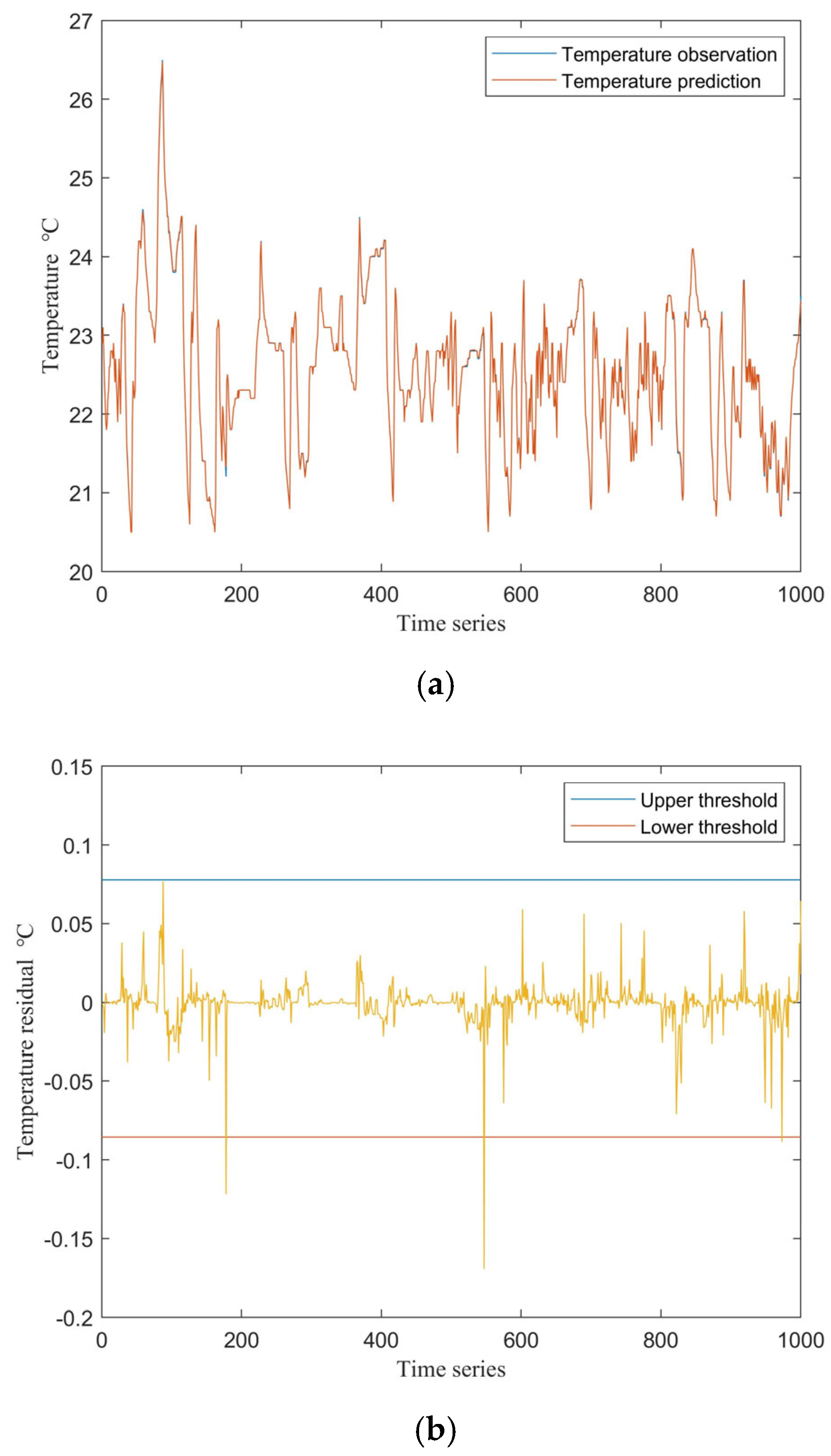
3.2. Model Comparison and Fault Detection Performance

Experimental data from one week in March were selected to evaluate the performance of the air conditioning control system models. A comparison between the conventional NSET model and the proposed PCA-NSET model clearly demonstrates the superior accuracy of the latter, as illustrated in Figure 5. As shown, the residuals and error fluctuations of the PCA-NSET model are significantly smaller than those of the conventional NSET model, indicating that the PCA-NSET model achieves higher prediction accuracy and better overall performance.

Although Figure 5 visually demonstrates the consistent reduction in residuals and volatility for the PCA-NSET model, detailed quantitative metrics such as mean residual or root mean square error (RMSE) were not calculated in this study due to current limitations in accessing the original numerical dataset. To further enhance the robustness of the results, future work will prioritize obtaining the complete dataset to enable calculation and reporting of key quantitative metrics, including RMSE and MAE, which are widely used in model performance evaluation. Nevertheless, the observed trend in the plotted results provides strong qualitative evidence of the superior performance of the PCA-NSET approach. Moreover, we have updated the figure captions in this section to provide more descriptive information on the key trends, thresholds, and practical implications, in order to better guide readers’ interpretation. Future work will include comprehensive quantitative comparisons as soon as the underlying data become available.

Experimental validation was conducted using data from 14 March to 22 March. During this eight-day period, the HVAC system operated normally for the first seven days, while a fault occurred on the eighth day. The established PCA-NSET model was applied to perform fault analysis on this dataset. For residual-based fault detection, the threshold was determined using the Laida criterion as described in Section 2.1. Specifically, for each monitored variable, the threshold was calculated as the mean plus or minus three standard deviations of the corresponding residuals under verified normal operating conditions. This ±3σ criterion was applied consistently across all analyses. In Figure 6 and Figure 7, the blue line indicates the upper threshold limit and the red line represents the lower threshold limit, both derived from the Laida criterion. This statistical approach provides an objective and reproducible standard for distinguishing between normal fluctuations and abnormal deviations. The predicted mixing room temperature and the corresponding temperature residuals for both the normal and fault periods are shown in Figure 6 and Figure 7, respectively.

As shown in Figure 6, when the air conditioning control system is operating normally, the model’s predicted values closely match the observed values, with residuals remaining within the threshold except for a few isolated points. In contrast, Figure 7 demonstrates that when a fault occurs in the system, there is a significant deviation between the predicted and observed values. The residuals increase sharply and consistently remain above the threshold. Therefore, by monitoring the residuals, effective fault prediction can be achieved; specifically, frequent exceedance of the threshold by the residuals can serve as an early warning indicator for system faults.

While the PCA-NSET model demonstrated perfect fault detection accuracy in this study, it is important to recognize that this result is closely related to the characteristics of the available dataset and the single fault scenario analyzed. In more complex or untested operational conditions, such as those involving multiple or overlapping faults, dynamic mode transitions, or greater environmental variability, the model’s performance and generalizability may be affected.

In addition, PCA is inherently a linear dimensionality reduction technique and may not fully capture nonlinear interactions present in some HVAC systems, potentially limiting the model’s applicability under highly nonlinear or rapidly changing process conditions. The NSET model’s accuracy and robustness are also sensitive to the selection and size of the process memory matrix: a large matrix can increase computational cost and risk overfitting, while a small matrix may reduce the model’s ability to represent the full spectrum of normal operational states.

Although this work cites alternative approaches—such as neural networks and various thresholding strategies—comprehensive quantitative comparisons with state-of-the-art benchmarks (e.g., [8,22]) were not conducted due to differences in datasets, evaluation metrics, and practical constraints. Despite these limitations, we have qualitatively compared our approach with representative literature and discussed the main advantages and disadvantages. Future research will aim to conduct systematic benchmarking studies using standardized datasets and evaluation protocols to enable direct, quantitative comparison with other advanced fault detection methods. Future research should focus on broader validation involving multiple fault types and diverse operating scenarios, as well as systematic benchmarking against other advanced fault detection methods to further substantiate the advantages and limitations of the proposed PCA-NSET framework.

4. Conclusions

This study investigated the operational status and fault detection of HVAC systems based on SCADA monitoring data. While most previous works focused on large-scale commercial or general industrial settings, this study demonstrates the applicability and benefits of PCA-NSET in the more stringent and regulated pharmaceutical manufacturing environment. After comprehensive data preprocessing, a predictive model was developed using a combination of PCA and NSET, and its performance was compared with that of the conventional NSET model. The results demonstrate that the PCA-NSET model achieves higher accuracy than the conventional NSET model, verifying the effectiveness of the proposed approach. Further analysis of SCADA data shows that, under normal operating conditions, the model’s residuals remain within a reasonable range, whereas during a fault, the residuals consistently exceed the threshold. These findings confirm that the proposed PCA-NSET model provides excellent performance in detecting faults in air conditioning control systems.

It should be noted, however, that this study did not quantify specific practical impacts such as downtime reduction or cost savings, as long-term operational and economic data were not available. The theoretical advancements of integrating PCA with NSET are promising, but require further benchmarking against a broader range of literature-reported methods to fully establish their generalizability and comparative advantage. Experimental validation in this work was limited to a one-week period containing a single real-world fault event, due to the rarity of faults and constraints of available industrial data. While this scenario provides a valuable demonstration of practical applicability, broader validation across multiple fault types, operational periods, and diverse datasets would further enhance the robustness and impact of the proposed approach. Future research will focus on addressing these limitations, including a comprehensive evaluation of practical benefits and systematic comparisons with alternative methods, as additional data become available.

The present study primarily focuses on fault detection during steady-state operation, as both PCA and NSET are most effective under quasi-stationary conditions. We acknowledge that system dynamics during equipment startup, shutdown, or mode transitions can significantly alter process variables and degrade the performance of conventional data-driven methods, potentially leading to false alarms or missed detections. Addressing these challenges requires either segmenting dynamic periods for separate analysis or developing advanced modeling techniques capable of capturing transient system behavior (e.g., using time-series analysis, recurrent neural networks, or adaptive thresholding). Future work will aim to extend the proposed methodology to explicitly account for such dynamic operating scenarios, thereby improving the comprehensiveness and robustness of the fault detection framework.

References

1. Dong, J.; Li, D.; Wei, Y.; Peng, K. A Novel Process Monitoring and Root Cause Diagnosis Strategy Based on Knowledge-Data-Integrated Causal Digraph for Complex Industrial Processes. IEEE Trans. Instrum. Meas. 2025, 74, 1–12. [Google Scholar] [CrossRef]
2. Luo, L.; Xie, L.; Su, H. Deep Learning with Tensor Factorization Layers for Sequential Fault Diagnosis and Industrial Process Monitoring. IEEE Access 2020, 8, 105494–105506. [Google Scholar] [CrossRef]
3. Simani, S.; Patton, R.J. Fault diagnosis of an industrial gas turbine prototype using a system identification approach. Control Eng. Pract. 2008, 16, 796–808. [Google Scholar] [CrossRef]
4. Uidhir, T.M.; Rogan, F.; Collins, M.; Curtis, J.; Gallachóir, B.P.Ó. Improving energy savings from a residential retrofit policy: A new model to inform better retrofit decisions. Energy Build. 2020, 209, 109656. [Google Scholar] [CrossRef]
5. Babayigit, B.; Abubaker, M. Industrial Internet of Things: A Review of Improvements Over Traditional SCADA Systems for Industrial Automation. IEEE Syst. J. 2024, 18, 120–133. [Google Scholar] [CrossRef]
6. West, S.R.; Ward, J.K.; Wall, J. Trial results from a model predictive control and optimisation system for commercial building HVAC. Energy Build. 2014, 72, 271–279. [Google Scholar] [CrossRef]
7. Es-sakali, N.; Zoubir, Z.; Idrissi Kaitouni, S.; Mghazli, M.O.; Cherkaoui, M.; Pfafferott, J. Advanced predictive maintenance and fault diagnosis strategy for enhanced HVAC efficiency in buildings. Appl. Therm. Eng. 2024, 254, 123910. [Google Scholar] [CrossRef]
8. Tun, W.; Wong, J.K.; Ling, S. Hybrid Random Forest and Support Vector Machine Modeling for HVAC Fault Detection and Diagnosis. Sensors 2021, 21, 8163. [Google Scholar] [CrossRef]
9. Taqvi, S.A.A.; Zabiri, H.; Tufa, L.D.; Uddin, F.; Fatima, S.A.; Maulud, A.S. A Review on Data-Driven Learning Approaches for Fault Detection and Diagnosis in Chemical Processes. ChemBioEng Rev. 2021, 8, 239–259. [Google Scholar] [CrossRef]
10. Venkatasubramanian, V.; Rengaswamy, R.; Yin, K.; Kavuri, S.N. A review of process fault detection and diagnosis: Part I: Quantitative model-based methods. Comput. Chem. Eng. 2003, 27, 293–311. [Google Scholar] [CrossRef]
11. Liu, L.; Huang, Y. HVAC Design Optimization for Pharmaceutical Facilities with BIM and CFD. Buildings 2024, 14, 1627. [Google Scholar] [CrossRef]
12. Smalls-Mantey, L.; Montalto, F. The seasonal microclimate trends of a large scale extensive green roof. Build. Environ. 2021, 197, 107792. [Google Scholar] [CrossRef]
13. Wang, S.; Zhang, Z.; Wang, P.; Tian, Y. Failure warning of gearbox for wind turbine based on 3σ-median criterion and NSET. Energy Rep. 2021, 7, 1182–1197. [Google Scholar] [CrossRef]
14. Aghili, S.A.; Khanzadi, M.; Haji Mohammad Rezaei, A.; Rahbar, M. Data-driven approach to fault detection for hospital HVAC system, Smart Sustain. Built Environ. 2024. ahead-of-print. [Google Scholar] [CrossRef]
15. Gao, Y.; Zhao, Y.; Hu, S.; Tahir, M.; Yuan, W.; Yang, J. A three-stage adjustable robust optimization framework for energy base leveraging transfer learning. Energy 2025, 319, 135037. [Google Scholar] [CrossRef]
16. Mirnaghi, M.S.; Haghighat, F. Fault detection and diagnosis of large-scale HVAC systems in buildings using data-driven methods: A comprehensive review. Energy Build. 2020, 229, 110492. [Google Scholar] [CrossRef]
17. Dey, M.; Rana, S.P.; Dudley, S. Smart building creation in large scale HVAC environments through automated fault detection and diagnosis. Future Gener. Comput. Syst. 2020, 108, 950–966. [Google Scholar] [CrossRef]
18. Qin, S.J. Statistical process monitoring: Basics and beyond. J. Chemom. 2003, 17, 480–502. [Google Scholar] [CrossRef]
19. Martínez, S.; Eguía, P.; Granada, E.; Moazami, A.; Hamdy, M. A performance comparison of multi-objective optimization-based approaches for calibrating white-box building energy models. Energy Build. 2020, 216, 109942. [Google Scholar] [CrossRef]
20. Somu, N.; Raman, G.M.R.; Ramamritham, K. A deep learning framework for building energy consumption forecast. Renew. Sustain. Energy Rev. 2021, 137, 110591. [Google Scholar] [CrossRef]
21. Kaib, M.T.H.; Kouadri, A.; Harkat, M.; Bensmail, A.; Mansouri, M. Improvement of Kernel Principal Component Analysis-Based Approach for Nonlinear Process Monitoring by Data Set Size Reduction Using Class Interval. IEEE Access 2024, 12, 11470–11480. [Google Scholar] [CrossRef]
22. Shittu, E.; Stojceska, V.; Gratton, P.; Kolokotroni, M. Environmental impact of cool roof paint: Case-study of house retrofit in two hot islands. Energy Build. 2020, 219, 110007. [Google Scholar] [CrossRef]
23. Afroz, Z.; Higgins, G.; Shafiullah, G.M.; Urmee, T. Evaluation of real-life demand-controlled ventilation from the perception of indoor air quality with probable implications. Energy Build. 2020, 219, 110018. [Google Scholar] [CrossRef]
24. Yuan, X.; Ma, C.; Chen, S. Research on Equipment Parameter Early Warning Based on GMM and NSET Optimization Algorithm. Kongzhi Gongcheng = Control Eng. China 2022, 29, 1058–1064. [Google Scholar] [CrossRef]
25. Bonvini, M.; Sohn, M.D.; Granderson, J.; Wetter, M.; Piette, M.A. Robust on-line fault detection diagnosis for HVAC components based on nonlinear state estimation techniques. Appl. Energy 2014, 124, 156–166. [Google Scholar] [CrossRef]
26. Kim, D.; Lee, J.; Do, S.; Mago, P.J.; Lee, K.H.; Cho, H. Energy Modeling and Model Predictive Control for HVAC in Buildings: A Review of Current Research Trends. Energies 2022, 15, 7231. [Google Scholar] [CrossRef]
27. Kazemi, H.; Yazdizadeh, A. Optimal state estimation and fault diagnosis for a class of nonlinear systems. IEEE/CAA J. Autom. Sin. 2020, 7, 517–526. [Google Scholar] [CrossRef]
28. Matetić, I.; Štajduhar, I.; Wolf, I.; Ljubic, S. A review of data-driven approaches and techniques for fault detection and diagnosis in HVAC systems. Sensors 2022, 23, 1. [Google Scholar] [CrossRef]
29. Ma, Y.; Borrelli, F.; Hencey, B.; Coffey, B.; Bengea, S.; Haves, P. Model predictive control for the operation of building cooling systems. IEEE Trans. Control Syst. Technol. 2012, 20, 796–803. [Google Scholar] [CrossRef]
30. Li, D.; Hu, G.; Spanos, C.J. A data-driven strategy for detection and diagnosis of building chiller faults using linear discriminant analysis. Energy Build. 2016, 128, 519–529. [Google Scholar] [CrossRef]
31. Na, W.; Zan, Q.; Gao, Y.; Guo, S.; Wang, Z. Real-time diagnosis and fault-tolerant control of a sensor single fault based on a data-driven feedforward-feedback control system. Processes 2022, 10, 1237. [Google Scholar] [CrossRef]
32. Toumi, R.; Kourd, Y.; Lefebvre, D. A novel fault detection approach based on multilinear sparse PCA: Application on the semiconductor manufacturing processes. Elektr. Turk. J. Electr. Eng. Comput. Sci. 2022, 30, 1586–1599. [Google Scholar] [CrossRef]
33. Windmann, S. Data-driven fault detection in industrial batch processes based on a stochastic hybrid process model. IEEE Trans. Autom. Sci. Eng. 2022, 19, 3888–3902. [Google Scholar] [CrossRef]
34. Tao, Y.; Shi, H.; Song, B.; Tan, S. A novel dynamic weight principal component analysis method and hierarchical monitoring strategy for process fault detection and diagnosis. IEEE Trans. Ind. Electron. 2020, 67, 7994–8004. [Google Scholar] [CrossRef]
35. Hamza, M.; Bafail, O.; Alidrisi, H. HVAC Systems Evaluation and Selection for Sustainable Office Buildings: An Integrated MCDM Approach. Buildings 2023, 13, 1847. [Google Scholar] [CrossRef]
36. Venkatasubramanian, V.; Rengaswamy, R.; Kavuri, S.N. A review of process fault detection and diagnosis: Part II: Qualitative models and search strategies. Comput. Chem. Eng. 2003, 27, 313–326. [Google Scholar] [CrossRef]
37. Lu, L.; Gao, X.; Shahnam, M.; Rogers, W.A. Open source implementation of glued sphere discrete element method and nonspherical biomass fast pyrolysis simulation. AIChE J. 2021, 67, e17211. [Google Scholar] [CrossRef]
38. Ali, U.; Shamsi, M.H.; Hoare, C.; Mangina, E.; O’Donnell, J. Review of urban building energy modeling (UBEM) approaches, methods and tools using qualitative and quantitative analysis. Energy Build. 2021, 246, 111073. [Google Scholar] [CrossRef]
39. Alghanmi, A.; Yunusa-Kaltungo, A. A whole-building data-driven fault detection and diagnosis approach for public buildings in hot climate regions. Energy Built Environ. 2024, 5, 911–932. [Google Scholar] [CrossRef]
40. Yun, W.; Hong, W.; Seo, H. A data-driven fault detection and diagnosis scheme for air handling units in building HVAC systems considering undefined states. J. Build. Eng. 2021, 35, 102111. [Google Scholar] [CrossRef]
41. Li, T.; Zhao, Y.; Zhang, C.; Luo, J.; Zhang, X. A knowledge-guided and data-driven method for building HVAC systems fault diagnosis. Build. Environ. 2021, 198, 107850. [Google Scholar] [CrossRef]
42. Ajagekar, A.; You, F. Quantum computing assisted deep learning for fault detection and diagnosis in industrial process systems. Comput. Chem. Eng. 2020, 143, 107119. [Google Scholar] [CrossRef]
Figure 1. Cumulative variance contribution rates of the principal components derived from SCADA system parameters.
Processes 13 02015 g001
Figure 2. Temperature variation curve of the mixing room during the study period.
Processes 13 02015 g002
Figure 3. Variation curve of the supply fan frequency during the study period.
Processes 13 02015 g003
Figure 4. Variation curves of residuals before and after data preprocessing.
Processes 13 02015 g004
Figure 5. Comparison of residuals between the conventional NSET model and the proposed PCA-NSET model.
Processes 13 02015 g005
Figure 6. Predicted mixing room temperature and residuals during the first seven days of operation: (a) Predicted and actual mixing room temperatures; (b) Residuals of the predicted mixing room temperature.
Processes 13 02015 g006
Figure 7. Predicted mixing room temperature and residuals on the eighth day of operation: (a) Predicted and actual mixing room temperatures; (b) Residuals of the predicted mixing room temperature.
Processes 13 02015 g007aProcesses 13 02015 g007b