Research on Cuttings Transport Behavior in the 32-Inch Borehole of a 10,000-Meter-Deep Well

Abstract

During the drilling processes of a 10,000-meter-deep well, cutting removal becomes difficult in the 32-inch borehole, which significantly increases downhole risks and affects drilling efficiency. To address this, a numerical simulation method based on the Eulerian two-fluid model was established for cuttings transport simulation in ultra-large boreholes. This method revealed the cuttings transport behavior in the 32-inch borehole of the SDCK1 well, analyzed the actual return velocity and the critical return velocity required for cuttings transport, and examined the cuttings transport characteristics near the bottom stabilizer. The results show that under the maximum flow rate of 160 L/s, the actual return velocity in the annulus is only 0.32 m/s, while the critical return velocity for 10 mm cutting particles is 0.57 m/s. Except for the stabilizer position, the actual return velocity throughout the entire well section is lower than the critical return velocity required for 10 mm cutting particles transport, which is one of the main reasons for the poor cutting removal in the wellbore. Near the bottom stabilizer, the annular flow is altered by the large outer diameter of the stabilizer, causing drilling fluid backflow and resulting in cuttings accumulation. The cuttings backflow and accumulation are more pronounced with the double stabilizer tool combination compared to the triple stabilizer tool combination. The small annular gap near the stabilizers makes it difficult for large cuttings to pass through, leading to blockages. A low annular return velocity and cuttings accumulation near the stabilizer are the primary reasons for poor cuttings removal in the 32-inch borehole.

1. Introduction

Deep reservoirs, characterized by abundant reserves and high productivity [1,2], have became one of the major oil and gas resources following deepwater [3,4] and unconventional resources [5,6]. China has actively devoted its efforts to deep oil and gas exploration, successfully developing ultra-deep oil and gas fields with an annual production capacity exceeding 10 million tons in the Tarim Basin [7,8] and Sichuan Basin [9]. To further explore the geological structures and development potential in ultra-deep formations, China has drilled two ultra-deep wells with vertical depths exceeding 10,000 m: SDTK1 in the Tarim Basin [10] and SDCK1 in the Sichuan Basin [11]. Drilling ultra-deep wells beyond 10,000 m poses enormous engineering and technical challenges. In particular, SDCK1 faces significantly complex formation pressure distributions [12,13]. SDCK1 is expected to encounter 14 different pressure gradients, with the maximum difference in adjacent formation pore pressure coefficients reaching 0.9, and it will penetrate 18 hydrocarbon-bearing formations with varying pressure coefficients. Consequently, a six-section, six-casing wellbore structure was adopted for SDCK1, with the upper second section featuring a 32″ borehole.

The borehole diameter has a remarkable impact on the drilling fluid flow behavior [14,15], which is directly reflected in the cutting transport. At the same flow rate, the annular return velocity of the drilling fluid in large-diameter boreholes decreases significantly, making it difficult for cuttings to return to the surface. A more severe challenge arises from the larger size of cuttings generated during large-diameter drilling, further complicating the upward transport of cuttings. During the drilling of the 32″ borehole in the second section of SDCK1, frequent cuttings transport inefficiencies led to sudden surges in standpipe pressure. Additionally, a large volume of cuttings was circulated out during shutdown periods, highlighting severe wellbore cleaning issues. A failure to remove cuttings promptly can lead to downhole incidents such as stuck pipe and formation fracture due to pressure surges [16,17]. Moreover, cuttings retained in the wellbore may undergo repeated fragmentation, generating excessive heat that poses a significant threat to downhole safety and reduces drilling efficiency [18,19,20].

However, current research on cuttings transport mechanisms and wellbore cleaning techniques mainly focuses on horizontal wells [21,22,23]. In terms of transport mechanisms, Nguyen and Rahman [24] proposed a three-layer model to predict cuttings transport states under high-declined and horizontal well conditions, categorizing cuttings into suspension, transition, and cuttings bed layers. Guan et al. [25] developed an optimization method for cuttings transport parameters in horizontal wells based on the multi-dimensional ant colony algorithm. Lu et al. [26] proposed a method for calculating the hydraulic extension length of horizontal sections based on the wellbore cleaning degree and analyzed the effects of related parameters. Zhang and Islam [27] established a real-time monitoring method for wellbore cleaning using a multi-point data-driven approach. Wang et al. [28] conducted experimental tests to establish the drag coefficient and settling velocity of irregular shale cuttings in horizontal wells. Yao et al. [29] investigated the relationship between the shale cuttings concentration and the risk of sticking in horizontal wells, suggesting that an optimal drill pipe rotation speed can improve wellbore cleaning and reduce sticking risks. As the wellbore depth and borehole size increase, renewed attention is being given to cuttings transport in vertical wellbores. For instance, Xu et al. [30] quantified the contributions of shear viscosity and fluid elasticity to terminal settling velocity and established the relationship between elastic drag coefficients and particle Reynolds numbers. Sun et al. [31] investigated cuttings transport in enlarged boreholes, emphasizing the need for specialized wellbore cleaning tools to enhance cuttings transport efficiency. However, research on cuttings transport in large-diameter vertical wellbores remains insufficient to fully elucidate the transport mechanisms and optimize wellbore cleaning efficiency.

In recent years, numerical simulations have become an essential tool for studying the cuttings transport mechanisms. This method can reveal the microscopic flow characteristics within complex fluid systems while also incorporating macroscopic trends derived from experimental data, thus providing a solid foundation for the validation of theoretical models and the improvement of empirical models. Currently, numerical simulation methods are primarily categorized into two types: the Eulerian–Eulerian method and the Eulerian–Lagrangian method [32]. The Eulerian–Eulerian method treats both the fluid phase and the particle phase as interpenetrating continuous media and simultaneously studies the motion of both phases within a Eulerian coordinate system. The Euler–Lagrange method, returning to the physical essence of the particle phase as a single discrete particle, determines the fluid phase by solving the Navier–Stokes equations. Prior studies have successfully validated this modeling framework for dense particle-laden flows in annular geometries, supporting its relevance to the current study [33,34]. While DEM-CFD coupling offers detailed particle-scale resolution, its computational cost is significantly higher. Given the focus on macroscopic flow behavior and engineering-scale analysis, the Eulerian–Eulerian model remains a suitable and widely accepted approach for this type of simulation.

To address this gap, this study employs computational fluid dynamics (CFD) numerical simulations to investigate the real-time cuttings transport behavior in the 32″ borehole of SDCK1, aiming to identify the key factors influencing cuttings transport efficiency and provide a theoretical basis for developing high-efficiency wellbore cleaning techniques for large-diameter boreholes.

2. Materials and Methods

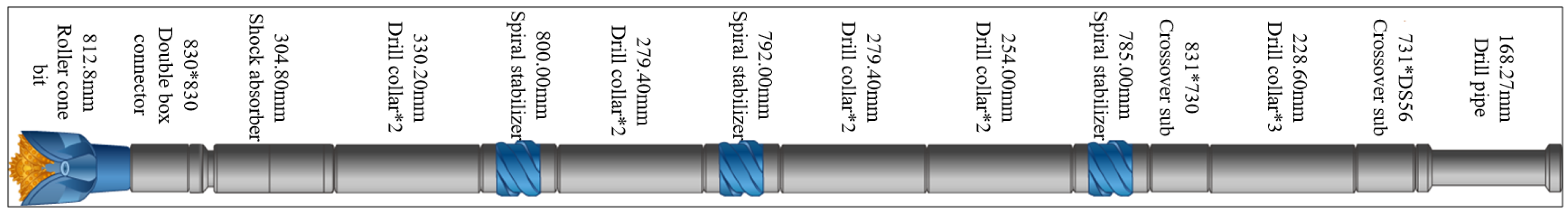
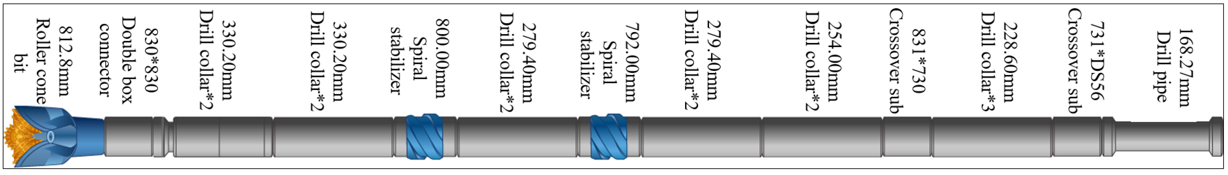
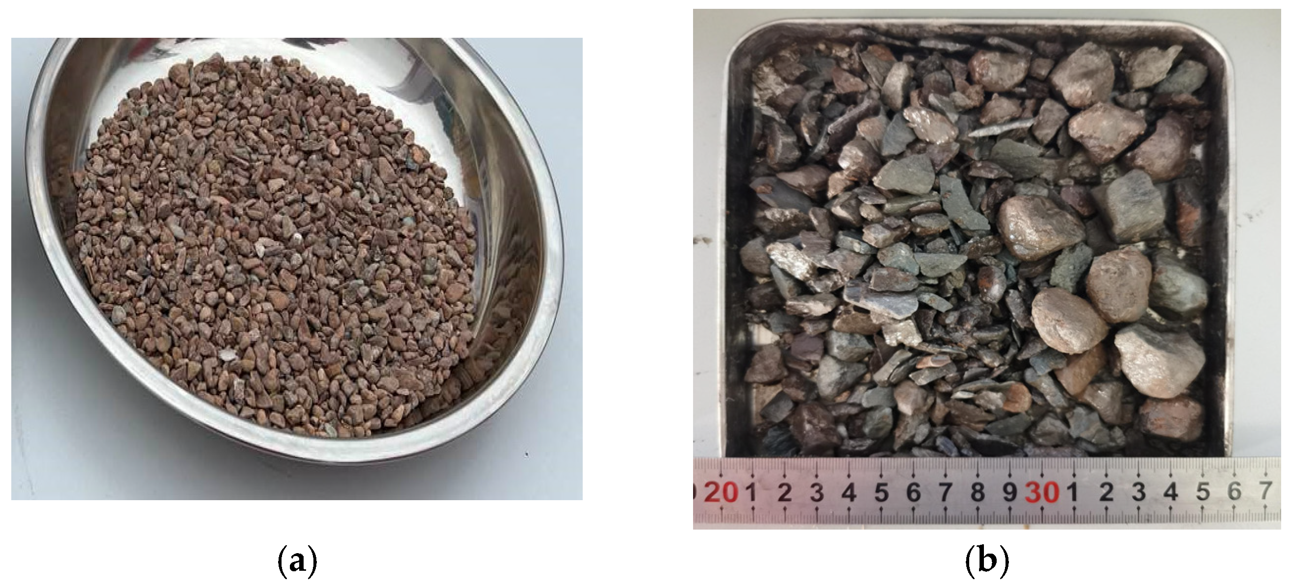
2.1. Description and Basic Parameters of Wellbore Cleaning in the 32-Inch Borehole

The SDCK1 well is an ultra-deep well in China, designed to reach a vertical depth of over 10,000 m, with the upper wellbore diameter reaching 32 inches. The SDCK1 well is drilled by a drilling rig equipped with a five-cylinder drilling pump, as shown in

Table 1. Specifications of the -Five-Cylinder Drilling Pump.

Cylinder Liner Diameter, mm	Max Stroke Rate, r/min	Maximum Discharge Pressure, MPa	Maximum Displacement, L/s
φ130	166	51.9	55.08
φ140	154	44.7	59.27
φ150	144	39.0	63.62
φ160	135	34.2	67.86
φ170	127	30.3	72.07
φ180	120	27.0	76.34

. During the drilling of the 32″ borehole, the maximum actual flow rate reaches 160 L/s. The actual drilling fluid density ranges from 1.10 to 1.27 g/cm³, the plastic viscosity ranges from 10 to 30 mPa·s, and the top drive rotational speed ranges from 55 to 95 r/min.

It is crucial to prevent wellbore deviation and ensure a straight trajectory in large-diameter upper sections. However, there are no available vertical drilling tools for the 32″ borehole. As a result, a combination of anti-deviation tools is used to control wellbore inclination. In the initial drilling stage, a three-stabilizer tower drilling tool combination is employed (as shown in Figure 1), with spiral stabilizers having outer diameters of Φ800 mm, Φ792 mm, and Φ785 mm. Due to poor cuttings removal, a dual-stabilizer drilling tool combination is adopted in the later drilling stage (as shown in Figure 2), with spiral stabilizers having outer diameters of Φ800 mm and Φ792 mm. Despite this, wellbore cleaning remains a significant issue during drilling.

The cuttings back to surface is shown in Figure 3. Under a 150 L/s flow rate, uniform and fine cutting particles are successfully circulated out. However, when the drilling mud has a heavy density and high consistency, a large number of uneven large-sized cutting particles are returned. Poor cuttings removal in the 32″ borehole severely increases downhole risks and affects drilling efficiency. On one hand, poor cutting removal repeatedly causes the riser pressure to spike to 25–26 MPa, significantly raising the risks of pipe stuck and wellbore loss. On the other hand, inadequate cuttings removal increases the number of tripping operations. The difficulty in returning cutting led to nine additional tripping operations. For a section of 470 m, the circulating time was 77.2 h, resulting in a circulation efficiency of only 10.8%, leading to low drilling efficiency.

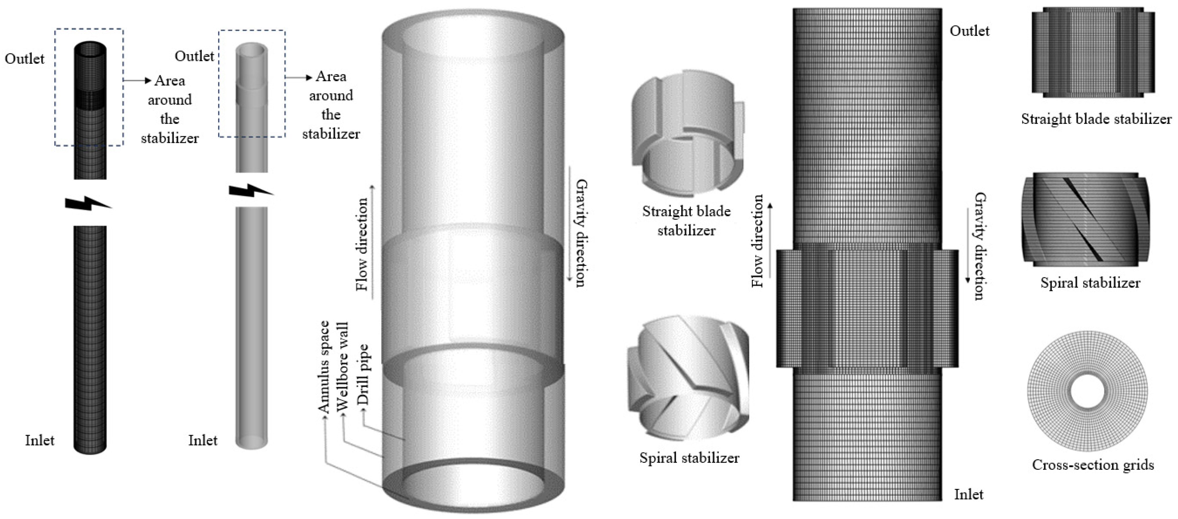
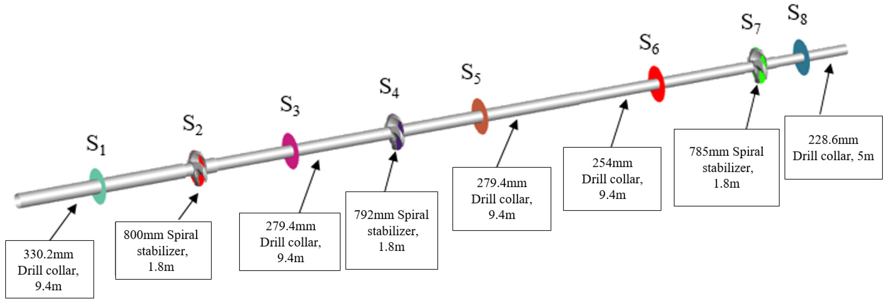
2.2. Geometric Model, Boundary Conditions, and Mesh Generation

A geometric model was established based on the real drilling data from the SDCK1 well, with the model representing a concentric annulus formed by different drill string combinations and the wellbore. Figure 4 shows the geometric model and grid division for the case of a double stabilizer drill string combination. The geometric parameters and numerical simulation parameters are shown in

Table 2. Geometric Parameters and Numerical Simulation Parameters.

No	Parameters	Value
1	Stabilizer Outer Diameter, mm	800/792
2	Well deviation angle, deg	0
3	Outer diameter of the drill string, mm	168.3
4	Inner diameter of the wellbore, mm	812.8/819.2
5	Drilling fluid density, kg/m3	1270
6	Fluid inlet velocity, m/s	0.20/0.26/0.32/0.38
7	Cuttings particle size, mm	2.0
8	Drilling fluid flow rate, L/s	100/130/160/190
9	Cuttings density, kg/m3	2500
10	Length of a single stabilizer, m	1.8
11	Stabilizer flow area, %	30/40/50/60
12	Apparent viscosity of drilling fluid, mPa·s	20
13	Inlet cuttings volume fraction % (corresponding to ROP 1.3 m/h)	3.6

. To reveal the cutting transport behavior near the bottom hole, numerical simulation contour plots were taken from the region near the stabilizers for analysis. For the boundary conditions at the entrance of the computational domain, a velocity inlet was selected, while a pressure outlet was chosen for the exit. The wall boundary condition was set as a no-slip wall. The SIMPLE algorithm was used with the pressure-coupled equation for semi-implicit methods. A second-order implicit scheme was applied for the transient equations. Additionally, the spatial discretization was set based on the least-squares gradient method, second-order pressure, and second-order upwind for momentum, and the modified turbulence viscosity was also set with a second-order upwind scheme.

Due to significant differences in the numerical simulation results caused by different grid sizes, four different grid sizes were selected for grid independence testing. The results are shown in

Table 3. Mesh Independence Test.

No	Model Grid Number	Rock Cuttings Volume Fraction	Relative Error
1	219,852	11.83%	-
2	294,195	10.99%	7.10%
3	347,340	10.51%	4.37%
4	467,512	10.43%	0.76%

. The initial value for the grid independence test was chosen as a grid number of 219,852. The relative error between the grid with 467,512 cells and the grid with 347,340 cells was 0.76%, indicating that the simulation results showed almost no change with grid numbers. Therefore, in this study, a hexahedral mesh with 340,000 cells was used to simulate the annular flow field during cutting transport. The annulus was discretized using a structured hexahedral mesh, and a local refinement technique was applied near the drill string and wellbore wall.

2.3. Governing Equations

In this study, a Eulerian–Eulerian two-fluid model was employed to describe the fluid–solid interactions in the numerical simulations. For the drilling fluid and cuttings in the annulus, continuity and momentum equations were established. The continuity equation is as follows [35,36]:

$${\displaystyle \frac{\partial \left({\alpha }_1{\rho }_1\right)}{\partial t}}+\nabla \cdot \left({\alpha }_1{\rho }_1{\mathit{u}}_1\right)=0$$

(1)

$${\displaystyle \frac{\partial \left({\alpha }_s{\rho }_s\right)}{\partial t}}+\nabla \cdot \left({\alpha }_s{\rho }_s{\mathit{u}}_s\right)=0$$

(2)

The momentum equation for the drilling fluid and cuttings in the annulus can be expressed as follows:

$${\displaystyle \frac{\partial \left({\alpha }_1{\rho }_1{\mathit{u}}_1\right)}{\partial t}}+\nabla \cdot \left({\alpha }_1{\rho }_1{\mathit{u}}_1{\mathit{u}}_1\right)=-{\alpha }_1\nabla p+\nabla \cdot \left({\alpha }_1\mathit{\tau }\right)+{\alpha }_1{\rho }_1\mathit{g}-\beta \left(v_1-v_s\right)$$

(3)

$${\displaystyle \frac{\partial \left({\alpha }_s{\rho }_s{\mathit{u}}_s\right)}{\partial t}}+\nabla \cdot \left({\alpha }_s{\rho }_s{\mathit{u}}_s{\mathit{u}}_s\right)=-{\alpha }_s\nabla p-\nabla p_s+\nabla \cdot \left({\alpha }_s\mathit{\tau }\right)+{\alpha }_s{\rho }_{s}g+\beta \left(v_1-v_s\right)$$

(4)

where the subscripts 1 and s represent the drilling fluid and cuttings, respectively; α is volume fraction,%; ρ is the density, g/cm³; u is the velocity vector, m/s; p is the pressure, Pa; p_s is the solid-phase pressure, kg/(m∙s²); τ is the stress tensor, Pa; g is the gravitational acceleration, Pa; and β is the interphase momentum transfer coefficient, Pa∙s/m².

The expression for the solid-phase pressure is as follows [37]:

$$p_s={\alpha }_s{\rho }_s{\Theta }_s+2{\rho }_s\left(1+e_{ss}\right){\alpha }_s^2{g}_{0,ss}{\Theta }_s$$

(5)

where e_ss is the coefficient of restitution for particle collisions; Θ_s is the granular temperature, m²/s²; and g_0,ss is the radial distribution function.

The radial distribution function can be expressed by the following equation [38]:

$$g_{0,ss}={\left[1-{\left({\displaystyle \frac{{\alpha }_s}{{\alpha }_{s,\max }}}\right)}^{{\displaystyle \frac{1}{3}}}\right]}^{-1}$$

(6)

where α_s,max is the packing limit, and α_s,max = 0.63.

The granular temperature can be expressed by the following equation [38]:

$${\Theta }_s={\displaystyle \frac{1}{3}}{u}_{s,i}{u}_{s,i}$$

(7)

In the two-fluid model, the solid-phase viscosity consists of collision viscosity, kinetic viscosity, and frictional viscosity, as expressed by Equation (8):

$${\mu }_s={\mu }_{s,\mathit{col}}+{\mu }_{s,\mathit{kin}}+{\mu }_{s,fr}$$

(8)

The expressions for collision viscosity, kinetic viscosity, and frictional viscosity are as follows [39]:

$${\mu }_{s,\mathit{col}}={\displaystyle \frac{4}{5}}{\alpha }_s{\rho }_s{d}_s{g}_{0,ss}\left(1+e_{ss}\right){\left[{\displaystyle \frac{{\Theta }_s}{\pi }}\right]}^{1/2}{\alpha }_s$$

(9)

$${\mu }_{s,\mathit{kin}}={\displaystyle \frac{10{\rho }_s{d}_s\sqrt{{\Theta }_s\pi }}{96{\alpha }_s\left(1+e_{ss}\right)g_{0,ss}}}{\left[1+{\displaystyle \frac{4}{5}}{g}_{0,ss}{\alpha }_s\left(1+e_{ss}\right)\right]}^2{\alpha }_s$$

(10)

$${\mu }_{s,fr}={\displaystyle \frac{p_s\sin \varphi }{2\sqrt{I_{2D}}}}$$

(11)

where d_s is the particle diameter, m; I_2D is the second invariant of the deviatoric stress tensor, m⁻⁴∙s⁻²; and Φ is the angle of internal friction, in degrees.

The volumetric viscosity refers to the resistance of particles to compression and expansion during flow [37], as expressed by Equation (12):

$${\lambda }_S={\displaystyle \frac{4}{3}}{\alpha }_S^2{\rho }_S{d}_s{g}_{0,ss}\left(1+e_{ss}\right){\left[{\displaystyle \frac{{\Theta }_S}{\pi }}\right]}^{1/2}$$

(12)

The momentum exchange coefficient between the solid and liquid phases is calculated using the Huilin–Gidaspow [40] model, which is a combination of the Ergun [41] model and the Wen & Yu [42] model. The equation is as follows:

$${\beta }_{\mathit{Huilin}-\mathit{Gidaspow}}=\phi {\beta }_{\mathit{Ergun}}+(1-\phi ){\beta }_{\mathit{Wen}\&\mathit{Yu}}$$

(13)

$$\varphi =\frac{\arctan [262.5\left({\alpha }_s-0.2\right)]}{\pi }+0.5$$

(14)

When α₁ ≤ 0.8,

$${\beta }_{\mathit{Ergun} }=150{\displaystyle \frac{{\alpha }_s\left(1-{\alpha }_1\right){\mu }_1}{{\alpha }_1{d}_s^2}}+1.75{\displaystyle \frac{{\rho }_1{\alpha }_s\left|\overrightarrow{u_s}-\overrightarrow{u_1}\right|}{d_s}}$$

(15)

When α₁ > 0.8,

$${\beta }_{\mathit{Wen}\&\mathit{Yu}}={\displaystyle \frac{3}{4}}{C}_D{\displaystyle \frac{{\alpha }_s{\alpha }_1{\rho }_1\left|\overrightarrow{u_s}-\overrightarrow{u_1}\right|}{d_s}}{\alpha }_1^{-2.65}$$

(16)

where C_D is the drag coefficient, which is dimensionless.

The calculation method of the drag coefficient is as follows:

$$C_D=\left\{\begin{array}{l}{\displaystyle \frac{24}{{\mathrm{Re}}_s}}\left(1+0.15{\mathrm{Re}}_s^{0.687}\right), {\mathrm{Re}}_s\le 1000\\ 0.44 ,{\mathrm{Re}}_s>1000\end{array}\right.$$

(17)

where Re_s is the particle Reynolds number, which is dimensionless.

The particle Reynolds number can be defined as Equation (18):

$$R{e}_s={\displaystyle \frac{{\rho }_1{d}_s\left|\overrightarrow{u_s}-\overrightarrow{u_1}\right|}{{\mu }_1}}$$

(18)

where d_s is the particle diameter, m.

The stress tensor for the cuttings and drilling fluid can be expressed as follows:

$$\overline{\overline{{\tau }_1}}={\mu }_1\left\{\left[\nabla \overrightarrow{u_1}+{\left(\nabla \overrightarrow{u_1}\right)}^T\right]-{\displaystyle \frac{2}{3}}\left(\nabla \cdot \overrightarrow{u_1}\right)\overline{\overline{I}}\right\}$$

(19)

$$\overline{\overline{{\tau }_s}}={\mu }_s\left[\nabla \overrightarrow{u_s}+{\left(\nabla \overrightarrow{u_s}\right)}^T\right]+\left({\lambda }_s-{\displaystyle \frac{2}{3}}{\mu }_s\right)\left(\nabla \cdot \overrightarrow{u_s}\right)\overline{\overline{I}}$$

(20)

where $\overline{\overline{I}}$ is the unit vector; μ₁ and μ_s are the viscosities of the fluid and solid phases, respectively, Pa·s; and λ_s is the solid-phase volumetric viscosity, Pa·s.

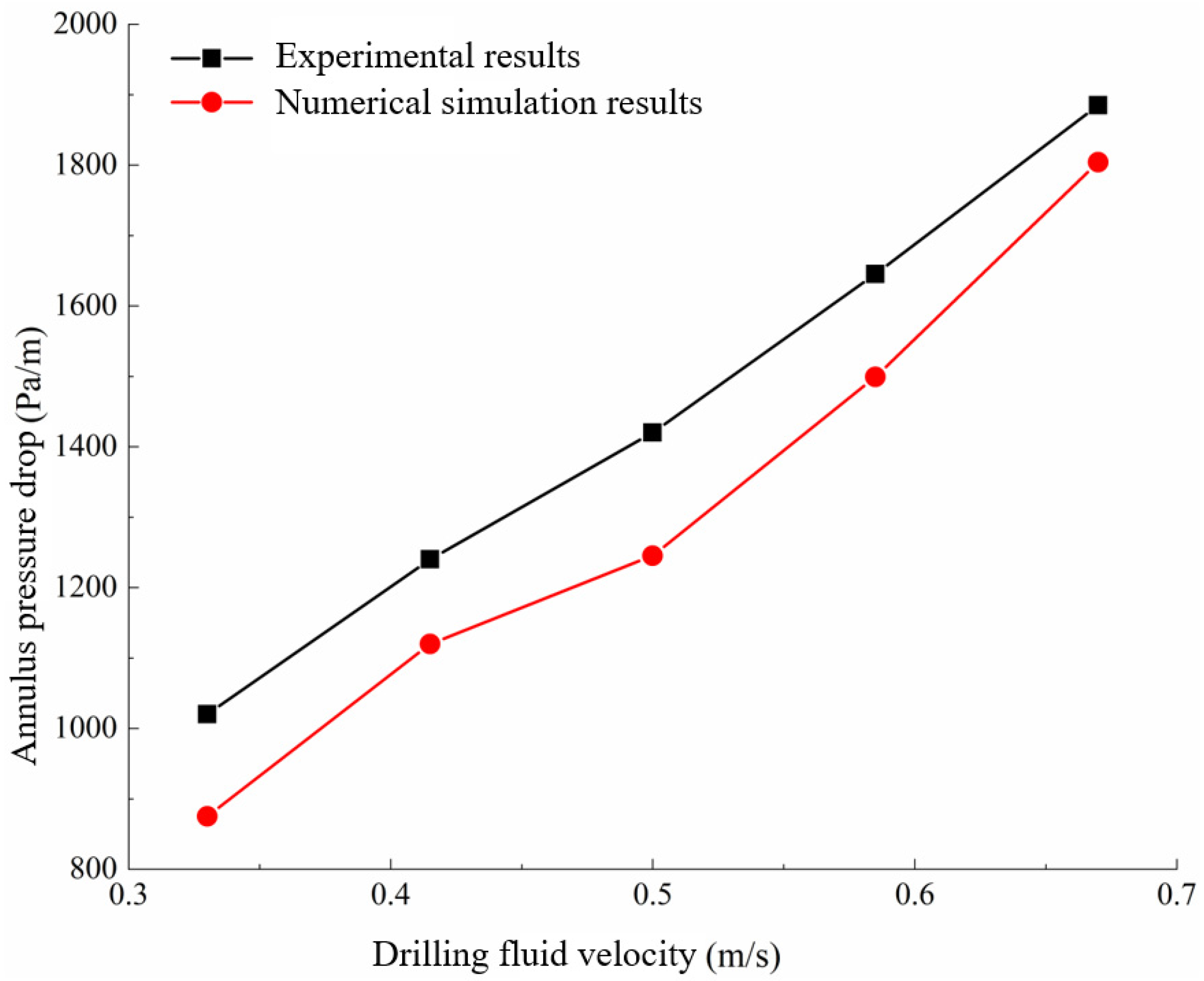
2.4. Model Validation

To ensure the validity of the numerical simulation results, the model’s prediction results were compared with experimental data. Due to the lack of experimental data on cuttings transport in large wellbores in the existing literature, the numerical model was validated using parameters identical to those in the reference experiment, which involved an annular inner diameter of 30 mm and an outer diameter of 44 mm. Figure 5 presents a comparison between the numerical simulation results for annular pressure drop at various drilling fluid flow rates under Eulerian two-fluid conditions. The experimental results are from Han [43]. An average error of 9.87% is between the numerical results and the experimental data, indicating a strong agreement. This confirms that the model can accurately predict cuttings transport under Eulerian two-fluid conditions.

3. Results and Discussion

3.1. Actual Annular Return Velocity and Critical Rock Carrying Return Velocity

To analyze whether the pump conditions and drilling fluid performance for the 32″ wellbore can meet the requirements for cuttings transport, the actual return speed and the critical return speed for cuttings under different particle sizes were analyzed. The critical annular return speed for cuttings transport in the drilling fluid is defined as the minimum return speed that can maintain the continuous upward movement of the cutting particles, as expressed by Equation (21) [44]:

$$u_{\min }={\displaystyle \frac{ROP}{\pounds \left[1-{\left(D_i/D_o\right)}^2\right]}}+k{u}_s$$

(21)

where, u_min is the critical return speed required for cuttings transport, m/s; ROP is the rate of penetration, taken as 1.3 m/h (the actual mechanical drilling speed for the 32″ wellbore); £ is the critical annular cutting volume fraction, set at 5%; D_o is the outer diameter of the drill string, mm; D_i is the inner diameter of the wellbore, with the upper casing section being 819.15 mm and the lower open hole section being 812.8 mm; K is the flow velocity correction factor, which is dimensionless and taken as 1.25; and u_s is the cuttings settling velocity, which is taken as 0.58 m/s based on actual measured cuttings data.

Using the model, the annular return velocity in the 32″ wellbore was calculated under a maximum flow rate of 160 L/s. Figure 6 presents a comparison between the calculated return velocity and the critical return velocity required for cuttings transport with particle sizes of 10 mm, 15 mm, 20 mm, and 25 mm. Numerical simulations were conducted to determine the minimum flow velocity required to transport cuttings of different sizes. The critical return velocity for cuttings transport was defined as the drilling fluid circulation velocity when the cuttings volume concentration in the wellbore reached 2%. The results indicate that variations in annular clearance lead to differences between the actual return velocity and the critical velocity required for cuttings transport for different particle sizes. In the upper casing section (0–60 m), where the annular clearance is the largest, the actual return velocity is at its minimum, reaching only 0.32 m/s. The critical return velocities required for cuttings transport in this section are 0.57 m/s, 0.73 m/s, 0.88 m/s, and 1.00 m/s for cuttings sizes of 10 mm, 15 mm, 20 mm, and 25 mm, respectively. Throughout the wellbore, except at the stabilizer location, the actual return velocity remains lower than the critical velocity required to transport 10 mm cuttings. This insufficient annular return velocity in the 32″ wellbore is one of the primary reasons for the poor cuttings removal.

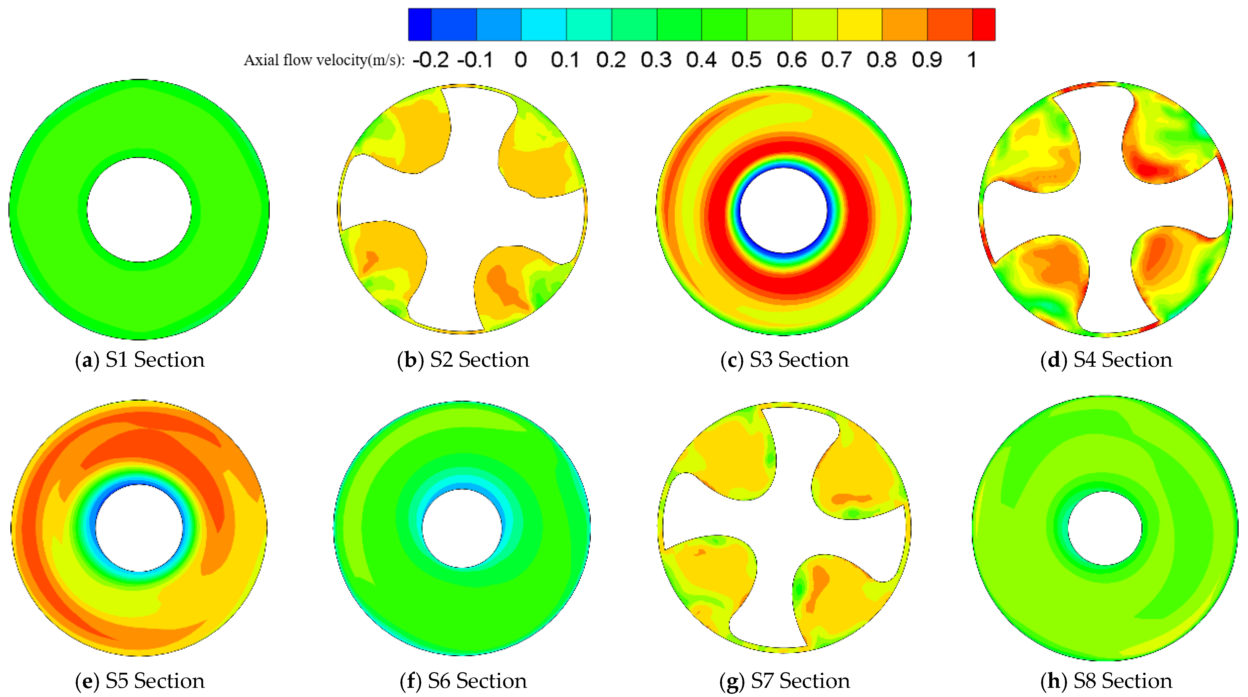
3.2. Cuttings Transport Characteristics near the Wellbore Bottom with a Three-Stabilizer BHA Configuration

To investigate the cuttings accumulation mechanism near the helical stabilizers, numerical simulations were conducted to analyze cuttings transport under two different bottom-hole assembly (BHA) configurations: a three-stabilizer assembly and a two-stabilizer assembly. The focus was on the axial velocity distribution in the annulus around the BHA. The simulation conditions were set based on field data: a laminar flow model, a drilling fluid density of 1.27 g/cm³, a cuttings density of 1.2 g/cm³, an initial cuttings concentration of 0.5%, a drilling fluid flow rate of 150 L/s, and a rotary speed of 90 r/min. Axial velocity analysis was conducted at eight different cross-sections along the bottom-hole assembly (Figure 7). The effective flow area at key locations, including the drill collars of varying diameters and three stabilizers, was examined to interpret the simulation results.

As shown in Figure 8, the presence of large-diameter helical stabilizers causes multiple abrupt changes in the annular flow area near the wellbore bottom, resulting in complex axial fluid velocity variations. The axial velocity remains relatively stable below the bottom stabilizer (0.34 m/s at Section S1) and above the top stabilizer (0.58 m/s at Section S8), with the return velocity being higher in the upper annulus compared to the lower section. At the stabilizer cross-sections, the reduced flow area leads to increased axial velocity, reaching approximately 0.8 m/s. The middle stabilizer experiences higher axial velocity compared to the other two stabilizers, but the velocity distribution remains non-uniform. In the annular space between adjacent stabilizers, the velocity distribution is also irregular, and reverse flow occurs near the drill string, particularly in the annular region near the middle stabilizer (Sections S3 and S5), where backflow is more pronounced. The analysis indicates that poor cuttings transport near the wellbore bottom in the three-stabilizer BHA configuration is primarily caused by two factors. First, the large-diameter stabilizers significantly alter the drilling fluid flow field, inducing backflow that leads to cuttings accumulation. Secondly, the narrow annular clearance around the stabilizers (as small as 6.4 mm in some regions) prevents the passage of large cuttings, resulting in cuttings blockage.

3.3. Cuttings Transport Characteristics near the Wellbore Bottom with a Two-Stabilizer BHA Configuration

Axial velocity analysis was conducted at seven different cross-sections along the bottom-hole assembly (Figure 9). The effective flow area was examined at key locations, including drill collars of varying diameters and two stabilizers, to interpret the simulation results.

As shown in Figure 10, although the two-stabilizer BHA has fewer abrupt diameter transitions compared to the three-stabilizer configuration, the axial fluid velocity distribution in the annulus still remains complex. Below the bottom stabilizer (Section S1, average velocity of 0.34 m/s) and above the top stabilizer (Sections S6 and S7, with average velocities of 0.44 m/s and 0.37 m/s, respectively), the axial velocity remains stable. The return velocity above the upper stabilizer is higher than that below the lower stabilizer, following a trend similar to the three-stabilizer configuration. At the stabilizer cross-sections, the reduced flow area leads to an increase in axial velocity, reaching approximately 0.8 m/s. The velocity at the upper stabilizer is higher than that at the lower stabilizer, but the distribution remains non-uniform. Due to the flow constriction caused by the stabilizers, the axial velocity near them exhibits extreme variation, with high-velocity jet regions (greater than 1.2 m/s) in the middle of the annulus, while reverse flow occurs near both the wellbore wall and the drill string. This backflow is particularly significant in the annular region near the upper stabilizer (Sections S3 and S5), where a large eccentric recirculation zone is observed. The analysis indicates that cuttings transport characteristics in the two-stabilizer BHA configuration are similar to those in the three-stabilizer configuration. However, the recirculation region near the upper stabilizer is larger, intensifying cuttings accumulation due to backflow.

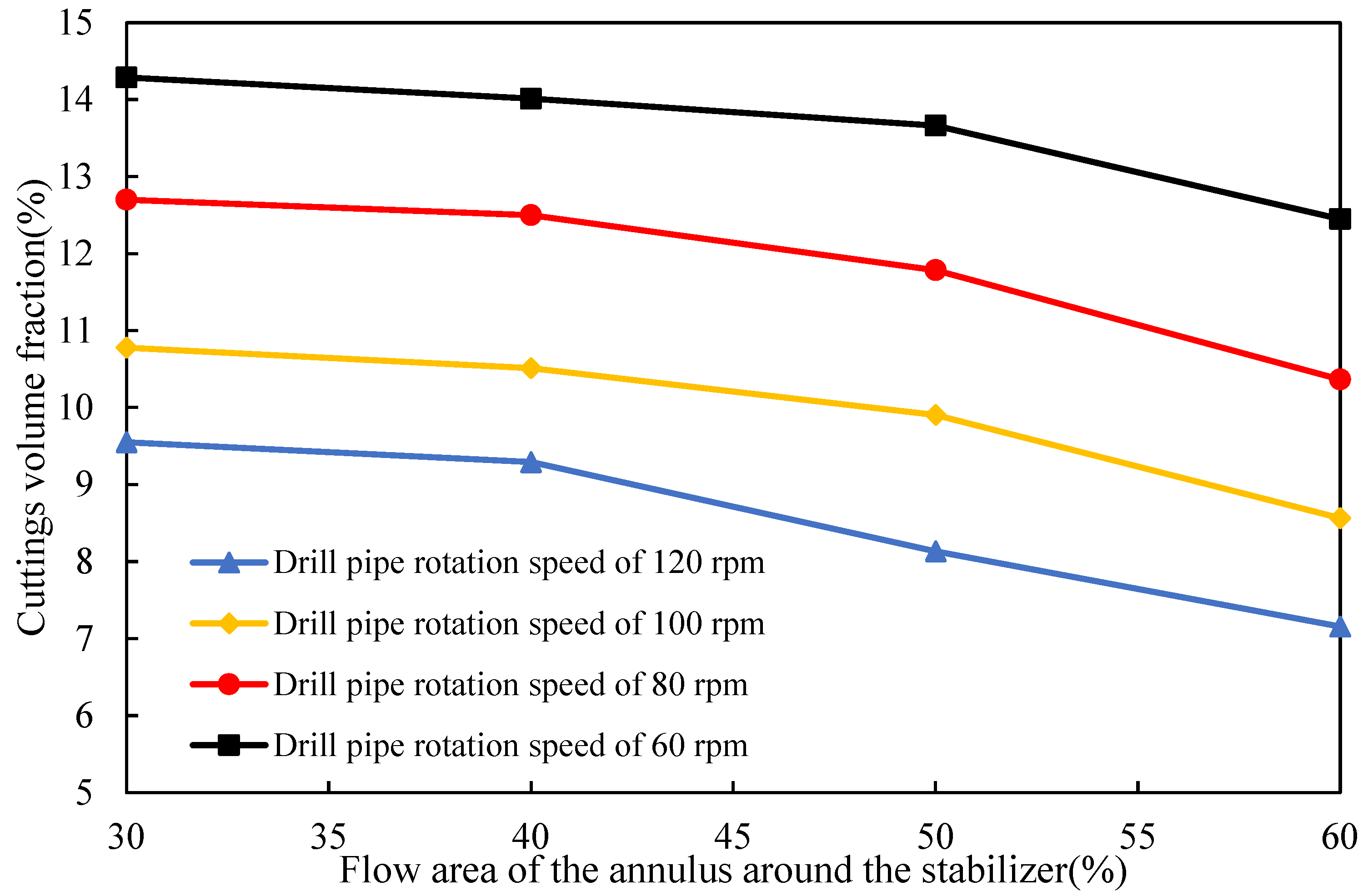
3.4. Impact of Stabilizers with Different Flow Areas

The flow area ratio of a stabilizer is defined as the proportion of the annular space between the stabilizer outer diameter and the wellbore inner diameter that allows fluid flow relative to the total annular space. Figure 11 illustrates the relationship between the stabilizer flow area ratio and cuttings volume fraction under different drill string rotational speeds. In general, as the stabilizer flow area increases, the drilling fluid velocity decreases, with the peak velocity occurring at the center of the stabilizer. When the stabilizer flow area ratio increases from 30% to 60%, the cuttings volume fraction decreases by 25.06% at drill string rotational speeds of 60 rpm. It is 20.53% at 80 rpm, 18.37% at 100 rpm, and 12.87% at 120 rpm, respectively. This indicates that a larger flow area allows cuttings to pass through the stabilizer region more easily, promoting their transport to the surface. However, increasing the stabilizer flow area weakens its functions in vertical hole deviation prevention and trajectory control. Moreover, an excessive flow area reduces the fluid velocity in the stabilizer region, weakening the lift force exerted on cuttings and slowing their transport. Therefore, selecting an appropriate stabilizer flow area requires a balance between effective hole cleaning and maintaining wellbore stability. When the stabilizer flow area ratio is 50%, the cuttings volume fractions at 60 rpm, 80 rpm, 100 rpm, and 120 rpm are 13.66%, 11.78%, 9.9%, and 8.13%, respectively. This demonstrates that, under identical conditions, the hole cleaning efficiency in ultra-deep large-diameter wells deteriorates significantly as the drill string rotational speed increases. However, the improvement in cuttings transport diminishes at higher rotational speeds. The rotational motion of the stabilizer blades transfers mechanical energy to the fluid, enhancing its tangential kinetic energy. Nevertheless, when the drill string rotational speed becomes too high, the incremental gain in vortex intensity caused by further speed increases diminishes.

4. Conclusions

(1)

A 32″ large-diameter borehole was used in the upper section of a 10,000-meter-deep well. During the drilling processes, severe hole-cleaning challenges emerged, significantly increasing the risks of pipe stuck and circulation lost. A numerical simulation method for cuttings transport in ultra-large boreholes was developed based on the Eulerian two-fluid model. This method effectively reproduces the cuttings transport process in a 32″ borehole of a 10,000-meter-deep well.

(2)

One of the primary reasons for inefficient cuttings transport in the 32″ borehole annulus is that the actual annular return velocity is lower than the critical velocity required for cuttings transport. The large-diameter stabilizers in the 32″ borehole annulus significantly alter the drilling fluid flow field, inducing fluid recirculation and causing cuttings accumulation near the wellbore bottom. This recirculation effect is more pronounced in the dual-stabilizer BHA configuration compared to the triple-stabilizer configuration.

(3)

To improve the cuttings transport efficiency in the 32″ wellbore, measures should be implemented simultaneously in three aspects: enhancing drilling parameters, optimizing drilling fluid properties, and refining the structure of helical stabilizers. At the same time, increasing the top drive speed can improve cuttings transport efficiency. The helical stabilizer alters the drilling fluid flow field, which is a major cause of cuttings accumulation near the wellbore bottom.

References

1. Xu, H.-L.; Xiang, S.-L.; Pei, D.-D.; Wu, X.-D.; Zhang, Z. Transient Collapse Failure Prediction of Production Casing After Packer Unsetting in High-Pressure and High-Temperature Deep Oil Wells. Processes 2025, 13, 839. [Google Scholar] [CrossRef]
2. Shen, W.; Ma, T.; Li, X.; Sun, B.; Hu, Y.; Xu, J. Fully coupled modeling of two-phase fluid flow and geomechanics in ultra-deep natural gas reservoirs. Phys. Fluids 2022, 34, 043101. [Google Scholar] [CrossRef]
3. Xie, R.; Zhang, L. A New Prediction Model of Annular Pressure Buildup for Offshore Wells. Appl. Sci. 2024, 14, 9768. [Google Scholar] [CrossRef]
4. Wang, C.; Cai, B.; Shao, X.; Zhao, L.; Sui, Z.; Liu, K.; Khan, J.A.; Gao, L. Dynamic risk assessment methodology of operation process for deepwater oil and gas equipment. Reliab. Eng. Syst. Saf. 2023, 239, 109538. [Google Scholar] [CrossRef]
5. Chen, Y.; Li, W.; Wang, X.; Wang, Y.; Fu, L.; Wu, P.; Wang, Z. Research and Application of Geomechanics Using 3D Model of Deep Shale Gas in Luzhou Block, Sichuan Basin, Southwest China. Geosciences 2025, 15, 65. [Google Scholar] [CrossRef]
6. Sheng, J.J. Critical review of field EOR projects in shale and tight reservoirs. J. Petrol. Sci. Eng. 2017, 159, 654–665. [Google Scholar] [CrossRef]
7. Jiao, S.; Li, W.; Li, Z.; Gai, J.; Zou, L.; Su, Y. Hybrid physics-machine learning models for predicting rate of penetration in the Halahatang oil field, Tarim Basin. Sci. Rep. 2024, 14, 5957. [Google Scholar] [CrossRef]
8. Jing, Y.; Wang, T.; Zhang, B.; Zheng, Y.; Li, X.; Lu, N. Safety Risk Analysis of Well Control for wellbore with sustained annular pressure and Prospects for Technological Development. Chem. Tech. Fuels Oil 2025, 61, 1676–1685. [Google Scholar] [CrossRef]
9. Zhang, D. Development prospect of natural gas industry in the Sichuan Basin in the next decade. Nat. Gas. Ind. B 2022, 9, 119–131. [Google Scholar] [CrossRef]
10. Wang, C.; Ming, C.; Chen, J.; Qu, H.; Wang, W.; Di, Q. Analysis of secondary makeup characteristics of drill collar joint and prediction of downhole equivalent impact torque of Well SDTK1. Petrol. Explor. Devel 2024, 51, 697–705. [Google Scholar] [CrossRef]
11. Zhu, X.; Li, K.; Li, W.; He, M.; She, C.; Tan, B. Drill string mechanical behaviors of large-size borehole in the upper section of a 10,000 m deep well. Nat. Gas. Ind. 2024, 44, 49–57. [Google Scholar]
12. Ou, C.; Li, C.; Huang, S.; Sheng, J.J. Remigration and leakage from continuous shale reservoirs: Insights from the Sichuan Basin and its periphery, China. AAPG Bull. 2019, 103, 2009–2030. [Google Scholar] [CrossRef]
13. Song, D.; Luo, X.; He, M. Development and Application of 812.8 mm PDC Bit for Myriameter Ultradeep Wells. China Petrol. Mach. 2025, 53, 31–36. [Google Scholar]
14. Mohammadzadeh, K.; Akbari, S.; Hashemabadi, S.H. Parametric study of cutting transport in vertical, deviated, and horizontal wellbore using CFD simulations. Pet. Sci. Technol. 2021, 39, 31–48. [Google Scholar] [CrossRef]
15. Erge, O.; Ozbayoglu, E.M.; Miska, S.Z.; Yu, M.; Takach, N.; Saasen, A.; May, R. Laminar to turbulent transition of yield power law fluids in annuli. J. Petrol. Sci. Eng. 2015, 128, 128–139. [Google Scholar] [CrossRef]
16. Cai, M.; He, M.; Tan, L.; Mao, D.; Xiao, J. Failure analysis of large-size drilling tools in the oil and gas industry. J. Energy Resour. Technol. 2024, 146, 073201. [Google Scholar]
17. Zhu, N.; Huang, W.; Gao, D. Numerical analysis of the stuck pipe mechanism related to the cutting bed under various drilling operations. J. Petrol. Sci. Eng. 2022, 208, 109783. [Google Scholar] [CrossRef]
18. Dehvedar, M.; Moarefvand, P.; Kiyani, A.R.; Mansouri, A.R. Using an experimental drilling simulator to study operational parameters in drilled-cutting transport efficiency. J. Min. Environ. 2019, 10, 417–428. [Google Scholar]
19. Mansoury, A.; Kiani, A.; Dehvedar, M.; Ameri, H. Well annulus cleaning while using stabilizer with an experimental flow loop and its cfd model. Arab. J. Sci. Eng. 2023, 48, 9413–9427. [Google Scholar] [CrossRef]
20. Sun, X.; Yan, T.; Li, W.; Wu, Y. Study on Cuttings Transport Efficiency Affected by Stabilizer’s Blade Shape in Vertical Wells. Open Petrol. Eng. J. 2013, 6, 7–11. [Google Scholar]
21. Li, X.; Gao, D.; Zhou, Y.; Zhang, H. Study on open-hole extended-reach limit model analysis for horizontal drilling in shales. J. Nat. Gas. Sci. Eng. 2016, 34, 520–533. [Google Scholar] [CrossRef]
22. Li, Z.; Yao, C.; Hu, K. Research and practice of horizontal wellbore cleaning technology. Xinjiang Oil Gas. 2022, 18, 48–53. [Google Scholar]
23. Chen, Y.F.; Zhang, H.; Wu, W.X.; Li, J.; Ouyang, Y.; Lu, Z.Y.; Dong, Z.X. Simulation study on cuttings transport of the backreaming operation for long horizontal section wells. Petrol. Sci. 2024, 21, 1149–1170. [Google Scholar] [CrossRef]
24. Nguyen, D.; Rahman, S.S. A three-layer hydraulic program for effective cuttings transport and hole cleaning in highly deviated and horizontal wells. SPE Drill. Complet. 1998, 13, 182–189. [Google Scholar] [CrossRef]
25. Guan, Z.; Liu, Y.M.; Liu, Y.W.; Xu, Y. Hole cleaning optimization of horizontal wells with the multi-dimensional ant colony algorithm. J. Nat. Gas. Sci. Eng. 2016, 28, 347–355. [Google Scholar] [CrossRef]
26. Lu, N.; Zhang, B.; Wang, T.; Fu, Q. Modeling research on the extreme hydraulic extension length of horizontal well: Impact of formation properties, drilling bit and cutting parameters. J. Pet. Explor. Prod. Tech. 2021, 11, 1211–1222. [Google Scholar] [CrossRef]
27. Zhang, F.; Islam, A. A pressure-driven hole cleaning model and its application in real-time monitoring with along-string pressure measurements. SPE J. 2023, 28, 1–18. [Google Scholar] [CrossRef]
28. Wang, Q.; Zhang, J.; Bi, C.; Liu, X.; Ji, G.; Yu, J. Study on settling characteristics of rock cuttings from terrestrial high clay shale in power-law fluid. Front. Energy Res. 2024, 12, 1370803. [Google Scholar] [CrossRef]
29. Yao, D.; Sun, X.; Zhang, H.; Qu, J. Experimental Study on Blocky Cuttings Transport in Shale Gas Horizontal Wells. Water 2025, 17, 1016. [Google Scholar] [CrossRef]
30. Xu, Z.; Song, X.; Zhu, Z. Development of elastic drag coefficient model and explicit terminal settling velocity equation for particles in viscoelastic fluids. SPE J. 2020, 25, 2962–2983. [Google Scholar] [CrossRef]
31. Sun, X.; Tao, L.; Qu, J.; Yao, D.; Hu, Q. Evaluating the effectiveness of cleaning tools for enhanced efficiency in reamed wellbore operations. Geoenergy Sci. Eng. 2025, 246, 213620. [Google Scholar] [CrossRef]
32. Yan, T.; Qu, J.; Sun, X.; Chen, Y.; Hu, Q.; Li, W.; Zhang, H. Numerical investigation on horizontal wellbore hole cleaning with a four-lobed drill pipe using CFD-DEM method. Powder Technol. 2020, 375, 249–261. [Google Scholar] [CrossRef]
33. Pang, B.; Wang, S.; Wang, Q.; Yang, K.; Lu, H.; Hassan, M.; Jiang, X. Numerical prediction of cuttings transport behavior in well drilling using kinetic theory of granular flow. J. Pet. Sci. Eng. 2018, 161, 190–203. [Google Scholar] [CrossRef]
34. Pang, B.; Wang, S.; Liu, G.; Jiang, X.; Lu, H.; Li, Z. Numerical prediction of flow behavior of cuttings carried by Herschel-Bulkley fluids in horizontal well using kinetic theory of granular flow. Powder Technol. 2018, 329, 386–398. [Google Scholar] [CrossRef]
35. Minakov, A.V.; Zhigarev, V.A.; Mikhienkova, E.I.; Neverov, A.L.; Buryukin, F.A.; Guzei, D.V. The effect of nanoparticles additives in the drilling fluid on pressure loss and cutting transport efficiency in the vertical boreholes. J. Pet. Sci. Eng. 2018, 171, 1149–1158. [Google Scholar] [CrossRef]
36. Yan, T.; Qu, J.; Sun, X.; Li, Z.; Li, W. Investigation on horizontal and deviated wellbore cleanout by hole cleaning device using CFD approach. Energy Sci. Eng. 2019, 7, 1292–1305. [Google Scholar] [CrossRef]
37. Lun, C.K.; Savage, S.B.; Jeffrey, D.J.; Chepurniy, N. Kinetic theories for granular flow: Inelastic particles in Couette flow and slightly inelastic particles in a general flowfield. J. Fluid. Mech. 1984, 140, 223–256. [Google Scholar] [CrossRef]
38. Ding, J.; Gidaspow, D. A Bubbling Fluidization Model Using Kinetic Theory of Granular Flow. AIChE J. 1990, 36, 523–538. [Google Scholar] [CrossRef]
39. Wolfshtein, M. The velocity and temperature distribution in one-dimensional flow with turbulence augmentation and pressure gradient. Int. J. Heat Mass Transfe 1969, 12, 301–318. [Google Scholar] [CrossRef]
40. Huilin, L.; Gidaspow, D.; Bouillard, J.; Wentie, L. Hydrodynamic simulation of gas–solid flow in a riser using kinetic theory of granular flow. Chem. Eng. J. 2003, 95, 1–13. [Google Scholar] [CrossRef]
41. Ergun, S. Fluid flow through packed columns. Chem. Eng. Prog. 1952, 48, 89–94. [Google Scholar]
42. Wen, C.Y. Mechanics of fluidization. Chem. Eng. Prog. 1966, 62, 100–111. [Google Scholar]
43. Han, S.M.; Hwang, Y.K.; Woo, N.S.; Kim, Y.J. Solid–liquid hydrodynamics in a slim hole drilling annulus. J. Petro Sci. Eng. 2010, 70, 308–319. [Google Scholar] [CrossRef]
44. Epelle, E.I.; Gerogiorgis, D.I. Transient and steady state analysis of drill cuttings transport phenomena under turbulent conditions. Chem. Eng. Res. Des. 2018, 131, 520–544. [Google Scholar] [CrossRef]
Figure 1. Three-Stabilizer Bottomhole Assembly in the Early Stage of 32″ Borehole Drilling.
Processes 13 02003 g001
Figure 2. 32″ Borehole Drilling Later Stage Dual-Stabilizer BHA Configuration.
Processes 13 02003 g002
Figure 3. Cuttings Returned from a 32″ Borehole During Actual Drilling: (a) Cuttings Returned at a 150 L/s Flow Rate; (b) Cuttings Return with Heavy High-Density Slurry Suspension.
Processes 13 02003 g003
Figure 4. Geometric Model and Mesh Generation.
Processes 13 02003 g004
Figure 5. Numerical Model Validation Results.
Processes 13 02003 g005
Figure 6. Return Velocity in the 32″ Wellbore Annulus at 160 L/s and Critical Return Velocity for Rock Cuttings of Different Sizes: (a) Three-Stabilizer Drill String Configuration; (b) Two-Stabilizer Drill String Configuration.
Processes 13 02003 g006
Figure 7. Selection of Cross-Sections for Axial Flow Velocity Analysis in the Annulus Near the Bottom of the Well with a Three-Stabilizer Tool Assembly.
Processes 13 02003 g007
Figure 8. Simulated results of axial fluid flow velocity at different annular cross-sections near the bottom of the well with a three-stabilizer tool assembly: (a) S1 Section; (b) S2 Section; (c) S3 Section; (d) S4 Section; (e) S5 Section; (f) S6 Section; (g) S7 Section; (h) S8 Section.
Processes 13 02003 g008
Figure 9. Selection of axial flow velocity analysis sections in the near-bottom annular space under the dual-stabilizer tool combination.
Processes 13 02003 g009
Figure 10. Simulation results of axial fluid flow velocity at different annular sections near the bottom with a dual-stabilizer tool combination: (a) S1 Section; (b) S2 Section; (c)S3 Section; (d) S4 Section; (e) S5 Section; (f) S6 Section; (g) S7 Section.
Processes 13 02003 g010
Figure 11. Relationship between stabilizer flow area and rock chip volume fraction at different drill string speeds.
Processes 13 02003 g011