Multi-Level Progressive Parameter Optimization Method for the Complex Process Industry

Abstract

The optimization of process parameters in the process industry usually faces challenges such as computational complexity caused by high-dimensional parameters. It is difficult for existing optimization methods to balance optimization accuracy with efficiency. Therefore, a multi-level progressive parameter optimization method for the complex process industry is proposed. Firstly, the importance evaluation method of parameters is constructed based on correlation analysis. By analyzing the correlation between process parameters and quality indicators, the importance rank of process parameters is realized. Then, a hierarchical method of process parameters based on importance evaluation is proposed. This method uses the sorted process parameters to divide the hierarchy, which lays a foundation for the subsequent multi-level progressive optimization. On this basis, a multi-level progressive modeling strategy is adopted to establish the nonlinear mapping relationship between process parameters and quality indicators layer by layer, and the optimal combination of process parameters is obtained with the improved particle swarm optimization. Finally, the data of a process production line is used for experimental verification. The verification results show that the proposed method can not only ensure the optimization accuracy but also significantly reduce the consumption of computing resources, which provides an efficient parameter optimization solution for the practical application of process industry.

1. Introduction

The process industry is an important part of the manufacturing industry, covering many key industries such as petrochemicals, metallurgy, building materials, light industry, and electric power [1]. These industries are not only the pillar of the national economy but also the key force to promote social development [2]. The technical process in the process industry is usually very complex, involving multi-dimensional process parameter coupling and interaction [3], which increases the complexity and difficulty of process parameter optimization. For example, small changes in any key process parameters in the process industry may lead to significant fluctuations in the reaction rate and product quality [4], thus affecting the stability of the entire production process [5]. Therefore, the optimization of process parameters in the process industry not only faces the challenge of multi-dimensional parameter adjustment but also needs to strike a balance between optimization accuracy and optimization efficiency. Above all, the construction of more efficient optimization methods [6] becomes urgent to improve production efficiency and achieve sustainable development [7].

In recent years, many experts and scholars have conducted in-depth research on the optimization of process parameters in the process industry. The main methods include the optimization method of extracting key parameters [8] and the overall optimization method considering global optimization [9]. Specifically, the optimization method of extracting key parameters is mainly to identify the key parameters with high correlation with quality indicators from many process parameters, thereby reducing the training cost of the prediction model. For example, Stanković et al. [10] emphasized the importance of key parameter extraction in process parameter optimization and introduced an intelligent initialization and greedy search strategy based on the suffix tree. These methods not only accelerate the convergence speed of the algorithm but also reduce the number of parameters that the operator needs to adjust, thereby significantly improving the efficiency of the manufacturing process and product quality. Jin et al. [11] rapidly screened and optimized the aluminum alloy deposition process parameters by using ultrasonic elastography technology, which greatly reduced the complexity and time cost of the experiment. This method allows efficient and suitable process parameter combinations to be obtained with a small sample size, thereby reducing the complexity of the optimization process parameters while improving efficiency. Ni et al. [12] developed a walnut shell-kernel separation device based on machine vision and improved efficiency and accuracy by optimizing key parameters. The improved YOLOv8n algorithm was used to enhance the recognition of small targets. The key parameters, such as air pressure, injection angle, and sorting height, were optimized by the Box-Behnken experimental design method, and the separation effect was improved by an artificial neural network. This method simplifies the experimental design, reduces the computational burden, and ensures the efficiency and accuracy of the separation process. Yin et al. [13] adopted the key parameter extraction strategy to simplify the training process of the prediction model for the optimization of the photothermoelectric effect of thermoelectric materials. This study analyzes the effects of carrier concentration and resonance wavelength and identifies the significant effects of these key parameters on the photothermal effect, thereby reducing the complexity of the parameter space in the optimization process. This method not only improves the photothermoelectric properties of the material but also effectively reduces the cost of model training and makes the experimental design more efficient. Wu et al. [14] proposed a multi-stage optimization framework combining artificial neural networks and computational fluid dynamics to improve the energy efficiency and mixing uniformity of the mixing tank. They extracted key parameters such as stirring speed and impeller diameter and optimized the model structure and initial weight by genetic algorithm, thereby improving the prediction accuracy and reducing the training cost. This method simplifies the parameter space and significantly improves the overall performance of the equipment. Song et al. [15] studied the fiber orientation and distribution optimization of ultra-high-performance fiber-reinforced concrete and analyzed the influence of key parameters such as pouring length, pouring height, and mixture viscosity on fiber behavior. By adjusting these key parameters, the parameter complexity in the concrete flow process can be reduced while maintaining the uniformity of fiber distribution. Fu et al. [16] studied the key process parameters of the CrAlSiWN coating. By extracting and optimizing the key parameters such as current, voltage, rotation speed, and duty cycle, the stability and wear resistance of the coating at high temperature were effectively improved. This optimization strategy not only improves the accuracy of the prediction model but also reduces the complexity and cost of model training by focusing on the key parameters affecting the coating performance. Although the optimization methods of extracting key parameters perform well in improving the prediction accuracy, there are still some limitations in practical applications. Since the key parameters extracted cannot completely replace the entire process data, some process parameters that have a sub-important impact on the quality indicators may be ignored. Therefore, these methods sacrifice optimization accuracy to improve optimization speed.

The overall optimization method considering global optimization is mainly to adapt to the complexity of process parameters and reduce their influence on the parameter optimization process by introducing more powerful prediction models or optimization methods. For example, Pfrommer et al. [17] used deep neural networks as surrogate models in their research and continuously optimized the model by iteratively introducing new data. This method can quickly identify potential optimal parameter combinations in high-dimensional parameter space, effectively reduce the influence of parameter complexity on the optimization process in the manufacturing process, and significantly improve optimization efficiency. By introducing the reinforcement learning algorithm based on Q-learning and the digital twin model of the Eagar-Tsai formula, Dharmadhikari et al. [18] proposed a new method to optimize the laser power and scanning speed parameters in the process of metal additive manufacturing. This study demonstrates how to reduce the influence of parameter complexity on the optimization process by improving the prediction model, thereby improving the efficiency and accuracy of process parameter optimization in the additive manufacturing process. By combining physical analysis and data-driven methods, Horr, A.M. [19], introduced machine learning-assisted hybrid techniques to optimize material process parameters in the production chain. This study demonstrates how to optimize analysis techniques through genetic algorithm symbolic regression and neural network training, thereby effectively reducing the impact of parameter complexity on the optimization process. In his research, Ge et al. [20] proposed a mathematical modeling and process parameter optimization method for carbon emissions of laser welding units. By establishing a mathematical model of carbon emissions of laser welding units and combining the Culture Algorithm and Ant Colony Algorithm to optimize process parameters, this study improves the methods of both predicting and optimizing process parameters, thereby reducing the influence of parameter complexity on the optimization process. Zhou et al. [21] constructed a surface roughness prediction model by using the response surface method and used the cuckoo search algorithm to optimize the multi-objective and multi-constrained cutting parameters. This method reduces dependence on parameter complexity when optimizing high-efficiency cutting process parameters, thereby ensuring processing quality and improving production efficiency. Xie et al. [22] proposed an improved optimization method combining a genetic algorithm and a BP neural network to improve the efficiency and accuracy of stamping process parameter optimization. This method improves the convergence speed and stability of the model by improving the selection, mutation, and crossover probability of the genetic algorithm and then enhances the overall optimization ability. The experimental results show that this optimization method effectively improves the forming quality and reduces the influence of parameter complexity on the optimization process. Zhu et al. [23] used the GWO-BPNN model based on grey wolf optimization and BP neural network to optimize process parameters. This method significantly improves the accuracy of predicting membrane separation performance and effectively reduces the influence of parameter complexity on experimental cost and uncertainty in the optimization process by reducing the number of experiments. Although the above-mentioned methods can deal with a large number of process parameters more effectively while maintaining the prediction accuracy so as to achieve more stable and efficient optimization results, these methods are apt to lead to high computational complexity when dealing with high-dimensional parameters, thereby prolonging the training time, making it difficult to meet the needs of rapid response in actual production.

In view of the above problems, this paper proposes a multi-level progressive parameter optimization method for complex process industries. Firstly, the importance of the parameters is sorted according to the correlation degree between the process parameters and the quality indicators, and then the sorted parameters are stratified by the random forest regression model. Based on this, a multi-level progressive modeling strategy is adopted to establish the nonlinear mapping relationship between process parameters and quality indicators layer by layer, and the optimal process parameter combination of each layer is obtained by combining the improved particle swarm optimization. In the process of constructing the mapping model, the optimal parameter combination obtained from the optimization of each layer is input as a constant to the next layer so as to realize the multi-level progressive optimization of process parameters. This method not only effectively reduces the influence of redundant parameters but also improves the optimization efficiency and accuracy. Finally, the data collected from a process production line is taken as an example for verification. The results show that the proposed method achieves a better balance between optimization accuracy and computational complexity. Compared with the existing optimization methods for extracting key parameters, the mean absolute error ($MAE$) and root mean square error ($RMSE$) of the proposed method are reduced by 42.05% and 42.71%, respectively, and the goodness of fit ($R^2$) is increased by 8.15%. Compared with the overall optimization method, the calculation time and the number of iterations of the proposed method are reduced by 63% and 49%, respectively. It provides an efficient parameter optimization solution for the practical application of the process industry.

2. Multi-Level Progressive Parameter Optimization Method for the Complex Process Industry

Aiming at the computational complexity caused by high-dimensional parameter optimization in the process industry, this paper proposes a multi-level progressive parameter optimization method for the complex process industry. The overall framework is shown in Figure 1. The method includes two main parts: a hierarchical model of process parameters based on importance evaluation and a multi-level progressive optimization model based on improved particle swarm optimization. Firstly, based on the pretreatment of process data, the correlation degree analysis method is used to calculate the correlation degree between process parameters and quality indicators, and the importance of process parameters is sorted accordingly. Subsequently, the random forest regression model was used to hierarchically process the sorted process parameters. Based on this, a multi-level progressive modeling strategy is adopted to establish the mapping model of each layer of process parameters and quality indicators layer by layer, and the optimal parameter combination is searched by combining the improved particle swarm optimization. In the process of constructing the mapping model, the optimal parameter combination obtained from the optimization of each layer is input as a constant to the next layer so as to realize the multi-level progressive optimization of process parameters.

(1) Parameter importance evaluation method based on correlation analysis: By quantitatively calculating the correlation between each process parameter and the quality index, the influence of each parameter on the quality index is systematically evaluated, and its importance is sorted. This method provides a scientific basis and decision support for the subsequent parameter stratification and optimization, thereby improving the stability of the process and product quality.

(2) Hierarchical model of process parameters based on importance evaluation: Based on the importance ranking results, the random forest regression model is used to stratify the process parameters. By analyzing the comprehensive evaluation index of the stability of the model, the process parameters are divided into different levels to reduce the impact of the complexity of the parameter dimension and improve the optimization efficiency.

(3) Multi-level progressive optimization model based on improved particle swarm optimization algorithm: The multi-level progressive modeling strategy is adopted to establish the mapping model of each layer of process parameters and quality indicators layer by layer, and the improved particle swarm optimization is used to search for the optimal combination of process parameters. In the process of constructing the prediction model, the optimal parameter combination of each layer is transmitted to the next layer as a fixed input so as to realize the multi-level progressive optimization of process parameters.

2.1. Hierarchical Model of Process Parameters Based on Importance Evaluation

2.1.1. Process Parameter Importance Evaluation Method Based on Correlation Analysis

Due to the significant difference in the influence of process parameters on quality indicators, it is very important to reasonably evaluate the importance of each process parameter to achieve effective quality control and process optimization. Therefore, this paper adopts the importance evaluation method of process parameters based on correlation analysis. This method systematically evaluates the influence of each parameter on the quality index by calculating the correlation between the process parameters and the quality index. Since the Pearson correlation coefficient can effectively reveal the correlation between the two [24], this study uses this coefficient to quantitatively analyze the correlation between process parameters and quality indicators. The Pearson correlation coefficient expression is as follows:

$$P\left(X,Y\right)={\displaystyle \frac{\sum _{I=1}^n\left(X_I-\overline{X}\right)\left(Y_I-\overline{Y}\right)}{\sqrt{\sum _{I=1}^n{\left(X_I-\overline{X}\right)}^2}\sqrt{{\left(Y_I-\overline{Y}\right)}^2}}}$$

(1)

In the formula, $X$ and $Y$ represent process parameters and quality indicators, respectively; $\overline{X}$ and $\overline{Y}$ represent the mean value of process parameters $X$ and quality indicators $Y$ respectively; and $P\left(X,Y\right)$ represents the correlation between them. The calculated correlation coefficient, $P\left(X,Y\right)$ reflects the correlation strength between the two, and its value range is $\left[-\mathrm{1,1}\right]$. The closer the value is to 1 or −1, the stronger the correlation is.

On the basis of calculating the correlation of each process parameter to the quality index, all the process parameters are sorted in descending order according to the correlation. The sorting process is as follows:

$$\left\{X_{\left(1\right)},X_{\left(2\right)},\cdots ,X_{\left(m\right)}\right\}=Sort\left\{P\left(X_1,Y\right),P\left(X_2,Y\right),\cdots ,P\left(X_m,Y\right)\right\}$$

(2)

In the formula, $X_{\left(1\right)}$ represents the process parameter with the strongest correlation with the quality index $Y$, and $X_{\left(m\right)}$ is the process parameter with the weakest correlation.

The sorted set of process parameters $\left\{X_{\left(1\right)},X_{\left(2\right)},\cdots ,X_{\left(m\right)}\right\}$ can lay the foundation for the subsequent hierarchical operation of process parameters according to its correlation with quality indicators.

2.1.2. Hierarchical Model of Process Parameters for High-Dimensional Processes

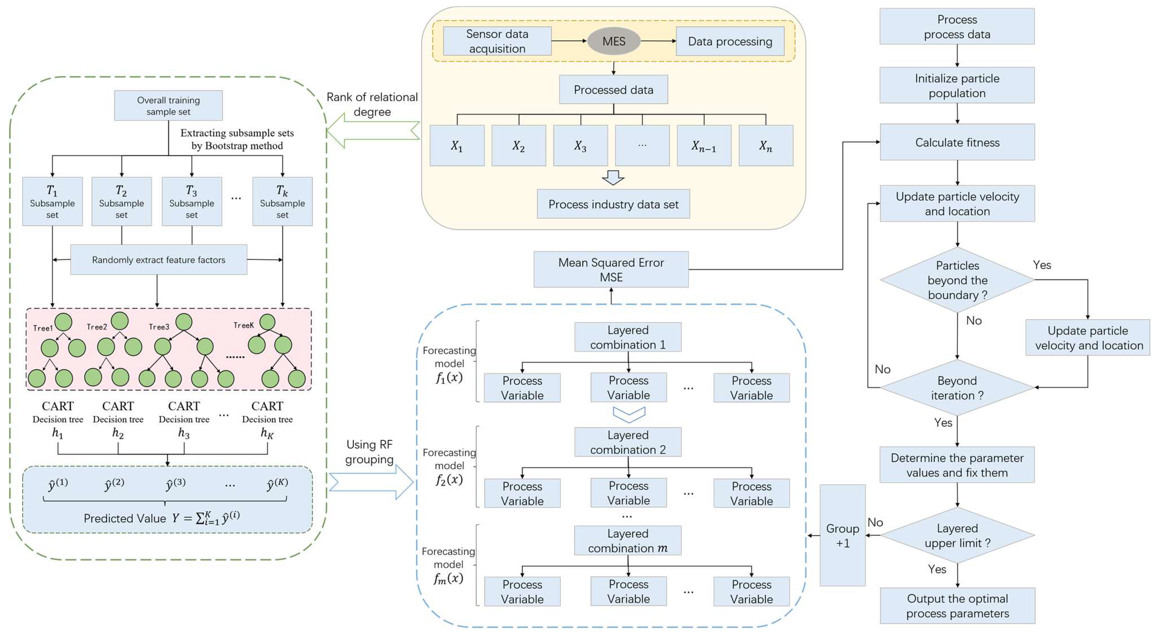
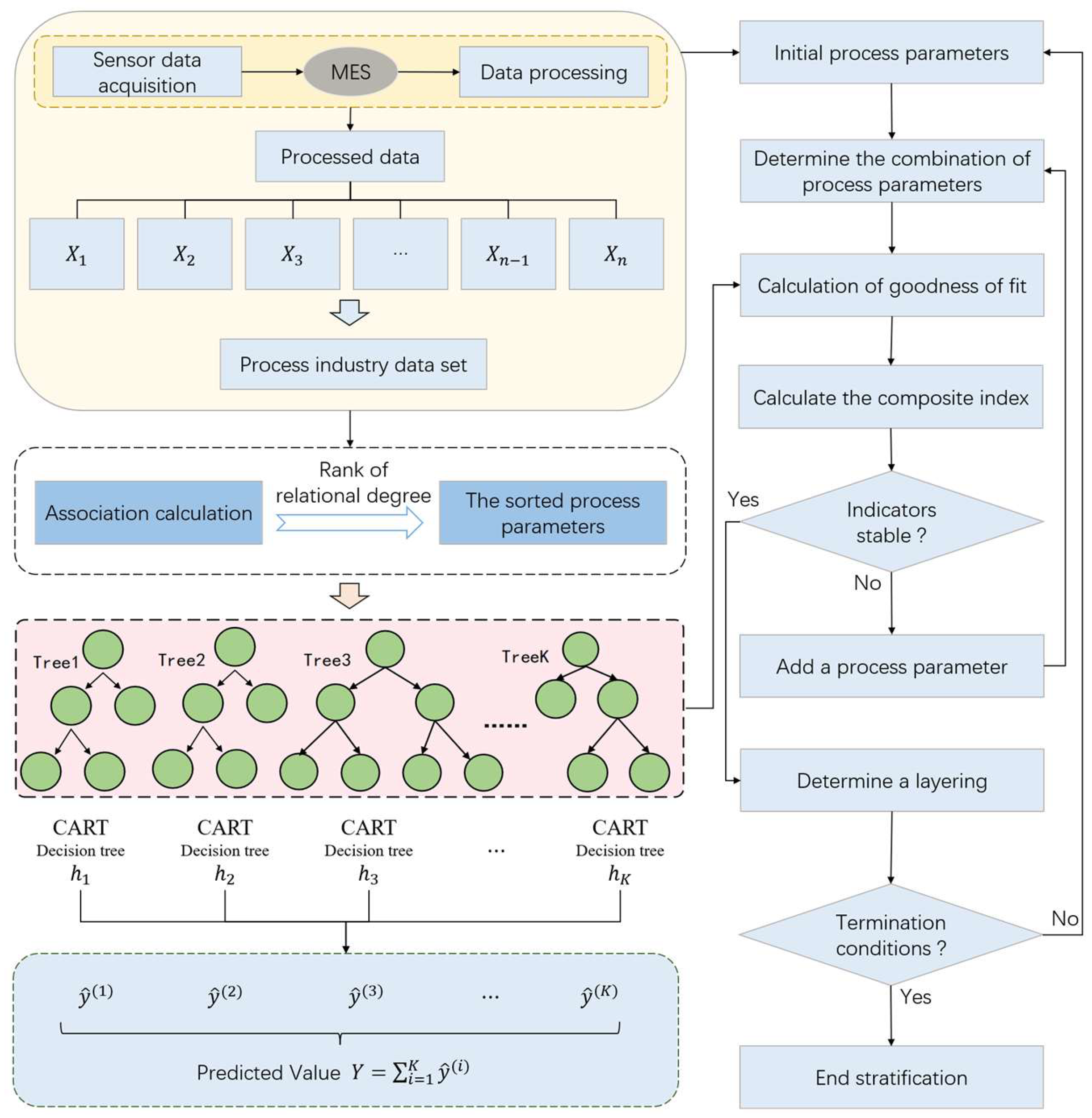
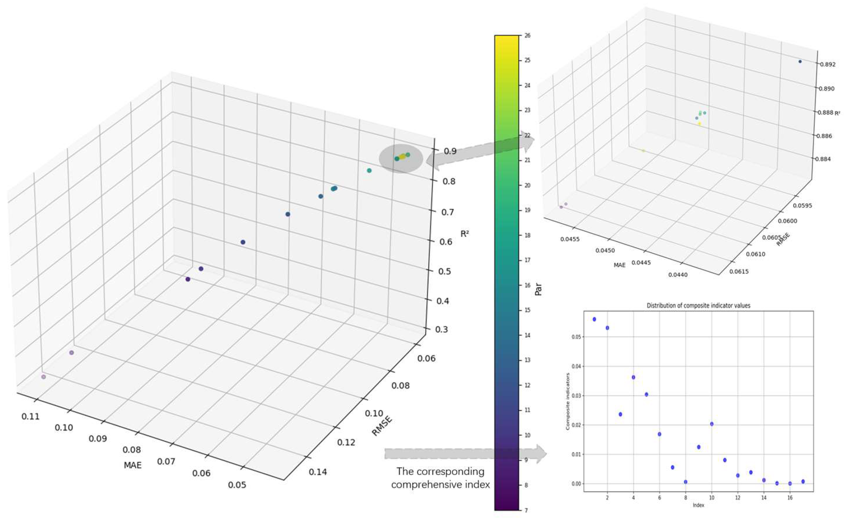
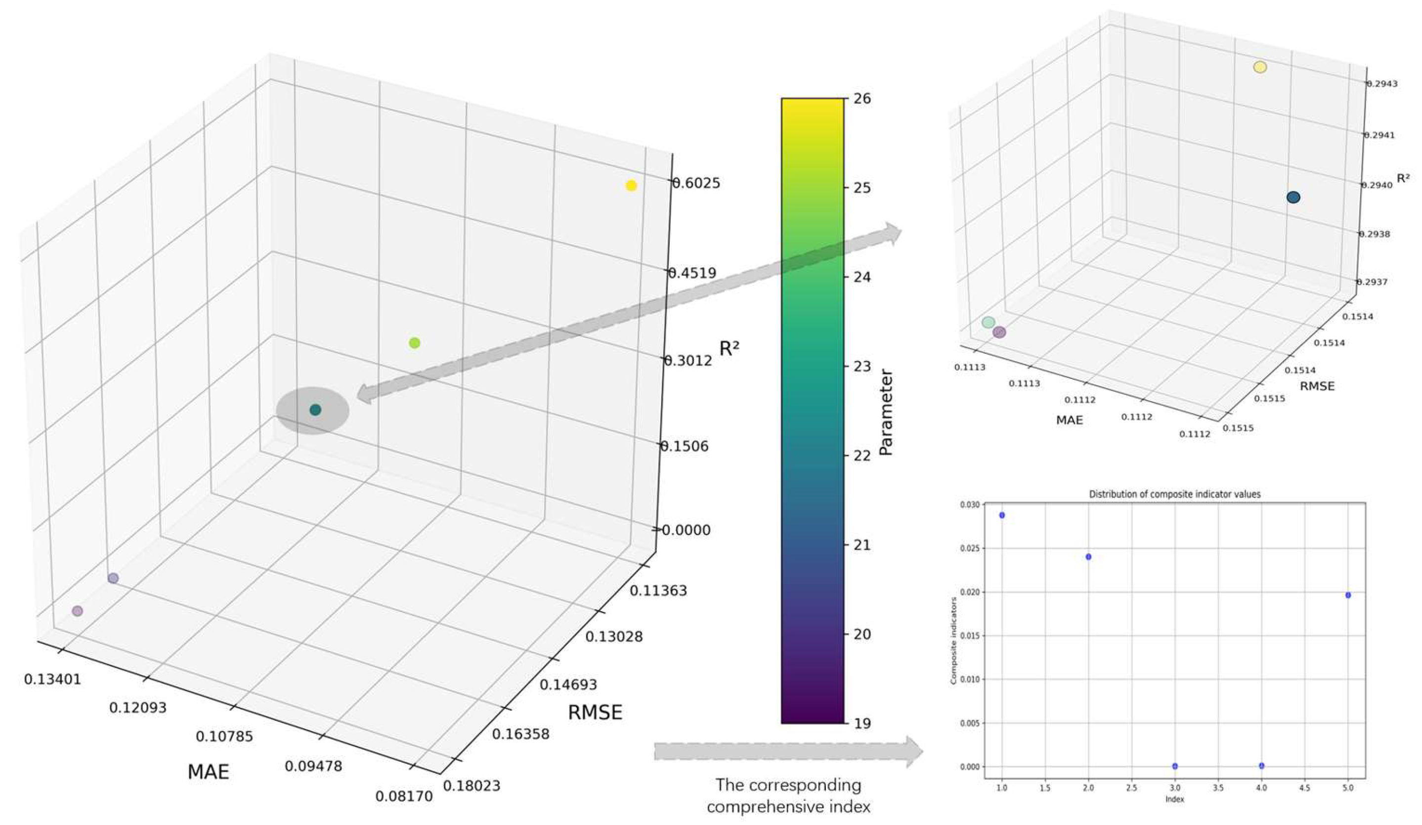
Since the dimension of process parameters is often high, the direct use of all sorted parameters for modeling or optimization will face significant computational complexity problems [25]. In order to effectively reduce the complexity of the model and improve the computational efficiency, a hierarchical model of process parameters based on importance evaluation is constructed. Firstly, the correlation degree between each process parameter and quality index is calculated by correlation degree analysis, and the process parameters are sorted according to the degree of correlation. Subsequently, the random forest regression model was used to hierarchically process the sorted process parameters. Among them, the process parameter stratification method is shown in Figure 2.

The specific processes are as follows:

(1) Data input: The process data set is composed of process parameters $X$ and quality index $Y$, which can be expressed as $D=\left\{X_{mn},Y_n\right\}$, where $X_{mn}$ represents the process parameters, $Y_n$ represents the quality index, $m$ represents the number of process parameters, and $n$ represents the number of samples in the process data set. On the basis of preprocessing the original data, $X_{mn}$ and $Y_n$ are used as the input of the hierarchical model of process parameters.

(2) Parameter importance assessment: The correlation degree between process parameters $X$ and quality index $Y$ is calculated so as to realize the sorting of process parameters according to the correlation degree. Its calculation is publicized as follows:

(3) Determine the initial process parameters: The process parameters with the largest correlation degree are selected as the initial process parameters, and the selected process parameters are temporarily divided into one layer.

(4) Model selection: Random forests can effectively capture complex nonlinear relationships and have excellent stability and robustness [26]. Therefore, this paper uses the random forest regression model to stratify the process parameters. Among them, the expression of the random forest objective function is

$${Obj}^{\left(k\right)}=\sum _{i=1}^{n}L\left(y_i,\widehat{y_i}\right)+\sum _{i=1}^n\Omega \left(f_k\right)$$

(3)

In the formula, $n$ represents the total number of samples, $y_i$ represents the true value, $\widehat{y_i}$ represents the model prediction value, $L\left(y_i,\widehat{y_i}\right)$ represents the loss function, $f_k$ represents the $k$-th tree, $\Omega \left(f_k\right)$ represents the regular term, the loss function, and the regular term are expressed as follows:

$$L\left(y_i,\widehat{y_i}\right)={\left(y_i-\widehat{y_i}\right)}^2$$

(4)

$$\Omega \left(f_k\right)=\gamma T+{\displaystyle \frac{1}{2}}\lambda \sum _{j=1}^T{\omega }_j^2$$

(5)

In the formula, $\gamma$ and $\lambda$ are penalty coefficients, $T$ is the number of leaf nodes, and $\omega$ is the weight of leaf nodes. Among them, the sum of the prediction results of the $k$-th decision tree is the prediction results of the random forest model. The calculation of the model prediction results is publicized according to Formula (5):

$${\widehat{y}}_i^{\left(k\right)}={\widehat{y}}_i^{\left(k-1\right)}+f_k\left(x_i\right)$$

(6)

In the formula, $x_i$ represents the $i$-th sample, $k$ represents the number of iterations, and $f_k\left(x_i\right)$ represents the weight of the $i$-th sample at the leaf nodes of the $k$-th decision tree.

(5) The calculation of goodness of fit ($R^2$): $R^2$ is used to measure the fitting ability of the model to the data [27]. The value of $R^2$ is between 0 and 1, and the closer to 1, the stronger the explanatory ability of the process parameters to the quality index.

$$R^2=1-{\displaystyle \frac{\sum _{j=1}^s{\left(y_{1,j}-y_{2,j}\right)}^2}{\sum _{j=1}^s{\left(y_{1,j}-\overline{y_2}\right)}^2}}$$

(7)

(6) Stability evaluation: In the process of model training, when adding a process parameter, it is necessary to directly observe the influence of the process parameters on the accuracy of the model. By analyzing the changes in the model accuracy under different parameter settings, it can be judged whether the model accuracy reaches a stable state within a certain range during the process of parameter increase. If not stabilized, then continue to increase the process parameters, and then repeat steps (3)~(6). If it has stabilized, the current process parameter combination is determined as a layer. Among them, in the stability judgment, the slope change rate is used as the main index to evaluate the change range of the model accuracy under the setting of adjacent parameters. When the number of process parameters is greater than 4, the calculation formula is as follows:

$$S_i=\left|{\displaystyle \frac{\left|E_{i+1}-E_i\right|-\left|E_{i+2}-E_{i+1}\right|}{E_i+E_{i+1}+E_{i+2}}}\right|$$

(8)

Here, $E_i$ represents the value of the accuracy of the i-th model, that is, the $R^2$ value representing the $i$-th. However, due to the possible correlation between some parameters during the model training process, the model accuracy fluctuates, which can be understood as a sudden change. In order to more effectively identify the stability of the trend, this paper introduces the mutation rate as an auxiliary index to measure the degree of mutation under different parameter levels. Its calculation formula is

$$M_i=\left|{\displaystyle \frac{E_i+E_{i+1}+E_{i+2}}{E_{i+3}}}\right|$$

(9)

Therefore, based on the above two indicators, the stability comprehensive index is introduced, and the overall stability of the model is quantitatively evaluated by the product of the slope change rate and the mutation rate. The calculation formula is as follows:

$$C_i=S_i·M_i$$

(10)

The stability of the model is judged by observing that the comprehensive index $C_i$ is less than 0.003 for the first time, and all subsequent values are always kept within 0.003. When this condition is satisfied, the model is considered to have reached a stable state. If the comprehensive index fails to remain below 0.003, skip this point and continue to observe the next point less than 0.003, and only when all the indicators remain within 0.003 after this point is the model judged to be stable. The selection of 0.003 as the threshold is based on in-depth analysis of experimental data and multiple experimental observations.

(7) Terminate condition checking: Determine whether the given termination condition is satisfied and determine the stratification result. If it is not satisfied, the process parameters that have completed the layering are deleted, and (3)~(7) is repeated.

2.2. Multi-Level Progressive Optimization Model of Process Parameters Based on Improved Particle Swarm Optimization Algorithm

Because the complex relationship between process parameters and quality indicators of each layer is still difficult to directly judge [28], it is impossible to directly construct the functional relationship model between them [29], so it is impossible to directly solve the optimal process parameter combination of each layer. In addition, considering the huge amount of process data in the process industry, it is impractical to use the exhaustive method to optimize the calculation.

Suppose that the process parameters are recorded as $x$, the number of process parameters is $X$, and the amount of data for each process parameter is $n$, that is:

$$x=\left\{x_1^n,x_2^n,\cdots ,x_X^n\right\}$$

(11)

$$x_X^n=\left\{x_X^1,x_X^2,\cdots ,x_X^n\right\}$$

(12)

It is assumed that the exhaustive method is used to optimize the whole process parameters directly. If the optimization combination is $G$ and the number of combinations is $N$, the combination and quantity formulas are as follows:

$$G=\left\{x_1^q,x_2^w,\cdots ,x_X^e\right\}$$

(13)

$$N=\prod \left(x_1^q,x_2^w,\cdots ,x_M^e\right)$$

(14)

$$q,w,\cdots ,e\in \left(\mathrm{1,2},\cdots ,n\right)$$

(15)

It can be seen from the above publicity that even if the values of $X$ and $n$ are extremely small, the calculation amount of process parameter optimization is also extremely large. Therefore, this paper introduces a hierarchical optimization strategy to reduce the computational burden. Assuming that the grouping is $M$, the process parameters are optimized hierarchically. The formula is as follows:

$$M=\left\{\begin{array}{c}{m}_1\\ m_2\\ ⋮\\ m_j\end{array}\right\}=\left\{\begin{array}{c}{x}_1^n,x_2^n,\cdots ,x_t^n\\ x_{t+1}^n,x_{t+2}^n,\cdots ,x_o^n\\ ⋮\\ x_{o+1}^n,x_{o+2}^n,\cdots ,x_M^n\end{array}\right\}$$

(16)

Among them, $m_1,m_2,\cdots ,m_j$ represent the process parameter group, $j$ represents the number of groups, $t$, $o-t$, $M-o$ represent the number of process parameters contained in different levels. The corresponding combination $G^{\prime }$ and number $N^{\prime }$ formulas are as follows:

$$G^{\prime }=\left\{\begin{array}{c}{x}_1^a,x_2^b,\cdots ,x_t^c\\ x_{t+1}^d,x_{t+2}^f,\cdots ,x_o^g\\ ⋮\\ x_{o+1}^h,x_{o+2}^k,\cdots ,x_M^l\end{array}\right\}$$

(17)

$$N^{\prime }=\prod \left(x_1^a,x_2^b,\cdots ,x_t^c\right)+\prod \left(x_{t+1}^d,x_{t+2}^f,\cdots ,x_o^g\right)+\prod \left(x_{o+1}^h,x_{o+2}^k,\cdots ,x_M^l\right)$$

(18)

$$\left\{\begin{array}{c}a,b,\cdots ,c\\ d,f,\cdots ,g\\ h,k,\cdots ,l\end{array}\right.\in \left(\mathrm{1,2},\cdots ,n\right)$$

(19)

Through the above analysis, the number of combinations is changed from the original multiplication to the accumulation of layers, so that the combination value is significantly reduced compared with $N$. This shows that the hierarchical optimization strategy can effectively reduce the complexity of optimization calculation and further proves the necessity of this method.

Although $N^{\prime }$ has been significantly reduced compared to $N$, it still has a huge amount of calculation, and direct use of exhaustive optimization will consume a lot of time and resources. Therefore, this paper introduces the particle swarm optimization algorithm [30] to search for the optimal parameter combination of each layer and accelerate the optimization process. In addition, in order to solve the problem that the optimization algorithm is difficult to take the accuracy of the algorithm into account while pursuing the convergence speed [31], the particle swarm optimization algorithm is improved as follows:

(1) The linear decreasing strategy of inertia weight is introduced to improve the convergence efficiency of the particle swarm optimization algorithm.

In the particle swarm optimization algorithm, the inertia weight $\omega$ s usually a fixed constant, which is used to control the search range of the particles. The larger inertia weight enables the particles to carry out extensive exploration in the search space, while the smaller inertia weight enhances the dependence of the particles on the historical optimal solution, thereby improving the local search accuracy. However, fixed inertia weight may lead to too scattered a search in the early stage and too concentrated a search in the later stage, which ultimately affects convergence efficiency. To this end, a linear decreasing strategy of inertia weight is introduced. The inertia weight $\omega$ is defined as

$${\omega }^{\left(s\right)}={\omega }_{max}-{\displaystyle \frac{{\omega }_{max}-{\omega }_{min}}{S}}\times s$$

(20)

In the formula, ${\omega }_{max}$ represents the maximum inertia weight; ${\omega }_{min}$ represents the minimum inertia weight; $S$ is the maximum number of iterations; $s$ is the current number of iterations. As the iteration progresses, the inertia weight gradually decreases, thereby enhancing the global search ability of the particles in the early stage of the algorithm and enhancing the local search ability in the later stage to avoid premature convergence.

(2) Adaptively adjust the acceleration factor to improve the global and local search balance of the particle swarm optimization algorithm.

In the particle swarm optimization algorithm, the acceleration factors $c_1$ and $c_2$ control the dependence of the particles on the individual optimal solution and the global optimal solution. Although a larger acceleration factor can accelerate the particles to move closer to the optimal solution, an excessively high acceleration factor may lead to excessive concentration of the search process, thus lacking sufficient diversity. Therefore, the dynamic adjustment of the acceleration factor is an important method to optimize the search process so that it can be dynamically adjusted with the increase in the number of iterations. The changes of $c_1$ and $c_2$ in each iteration should follow:

$$c_1^{\left(s\right)}=c_{1max}+{\displaystyle \frac{c_{1max}-c_{1min}}{S}}\times s$$

(21)

$$c_2^{\left(s\right)}=c_{2max}-{\displaystyle \frac{c_{2max}-c_{2min}}{S}}\times s$$

(22)

In the formula, $c_{1max}$ and $c_{2max}$ represent the corresponding maximum acceleration factor, $c_{1min}$ and $c_{2min}$ represent the corresponding minimum acceleration factor. Specifically, in the early stage of the search, the $c_1$ value is small, which helps the particles to perform global search, thereby avoiding premature convergence. As the iteration progresses, the $c_1$ value gradually increases, which enhances the dependence of the particles on the best position of the individual, thereby promoting the refinement of the local search. In contrast, in the early stage of the search, the $c_2$ value is larger, which promotes the particle to move closer to the global optimal position; as the iteration progresses, the $c_2$ value gradually decreases, reducing the dependence of the particles on the global optimal position and promoting a more concentrated local search. Through dynamic adjustment, a good balance between global search and local search is found so as to improve the search efficiency of the algorithm.

(3) The search position of particles is limited to ensure that the particle swarm optimization algorithm searches in the feasible solution space.

In the problem of high-dimensional parameter optimization, particles may move to infeasible regions. In order to ensure that the particles are always in the feasible solution space, the position of the particles is constrained so that the position of the particles is always kept within a reasonable range. The constraint expression is as follows:

$$h_i^{s+1}=\mathrm{m}\mathrm{a}\mathrm{x}\left(min\left(h_i^{s+1},h_{max}\right),h_{min}\right)$$

(23)

In the formula, $h_i^{s+1}$ represents the particle position, $h_{min}$ represents the lower limit of particle search, and $h_{max}$ represents the upper limit of particle search. In this way, the position of the particles will always be limited to the range of $\left[h_{min},h_{max}\right]$, preventing the particles from jumping out of the effective search area, thus ensuring the stability and effectiveness of the search process.

Through the above description, it can be seen that the search process of particles is dynamically optimized through the linear decrease in inertia weight, the adaptive adjustment of acceleration factor, and the restriction of particle search position, thus forming an improved particle swarm optimization algorithm. In the early stage of the algorithm, the population can enhance the global search ability and expand the search range, while in the later stage, the local search ability is enhanced and the convergence speed is accelerated, which helps to find the optimal solution more effectively.

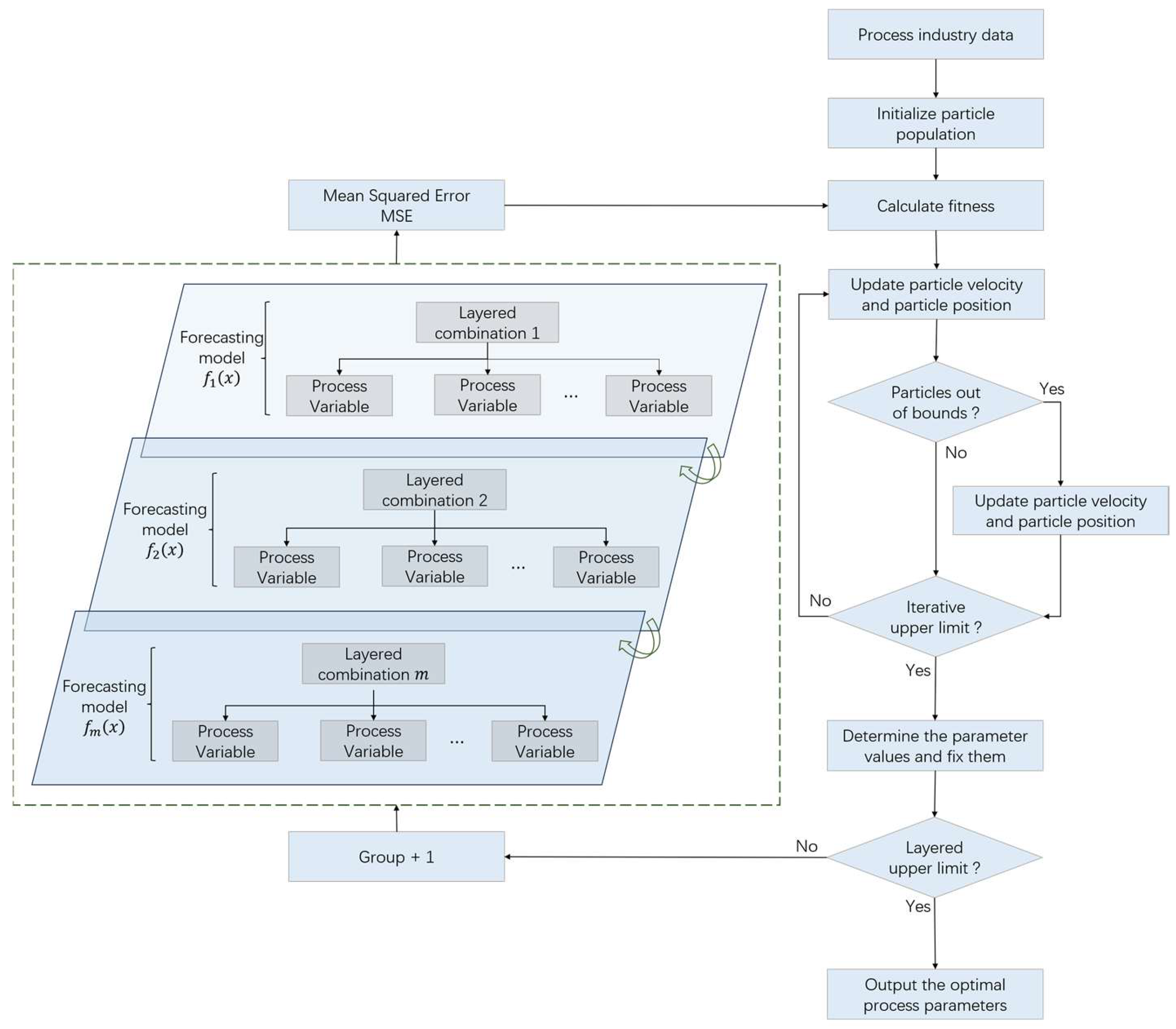
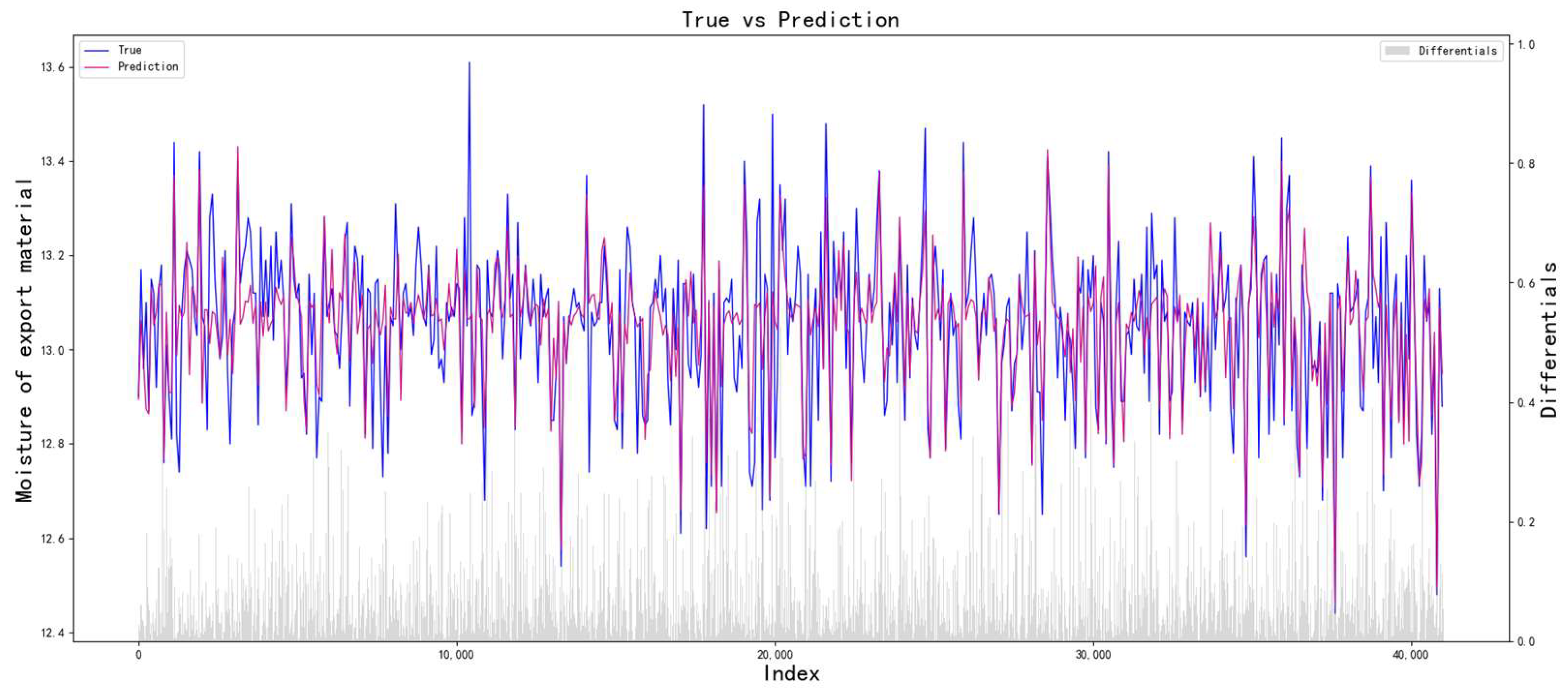
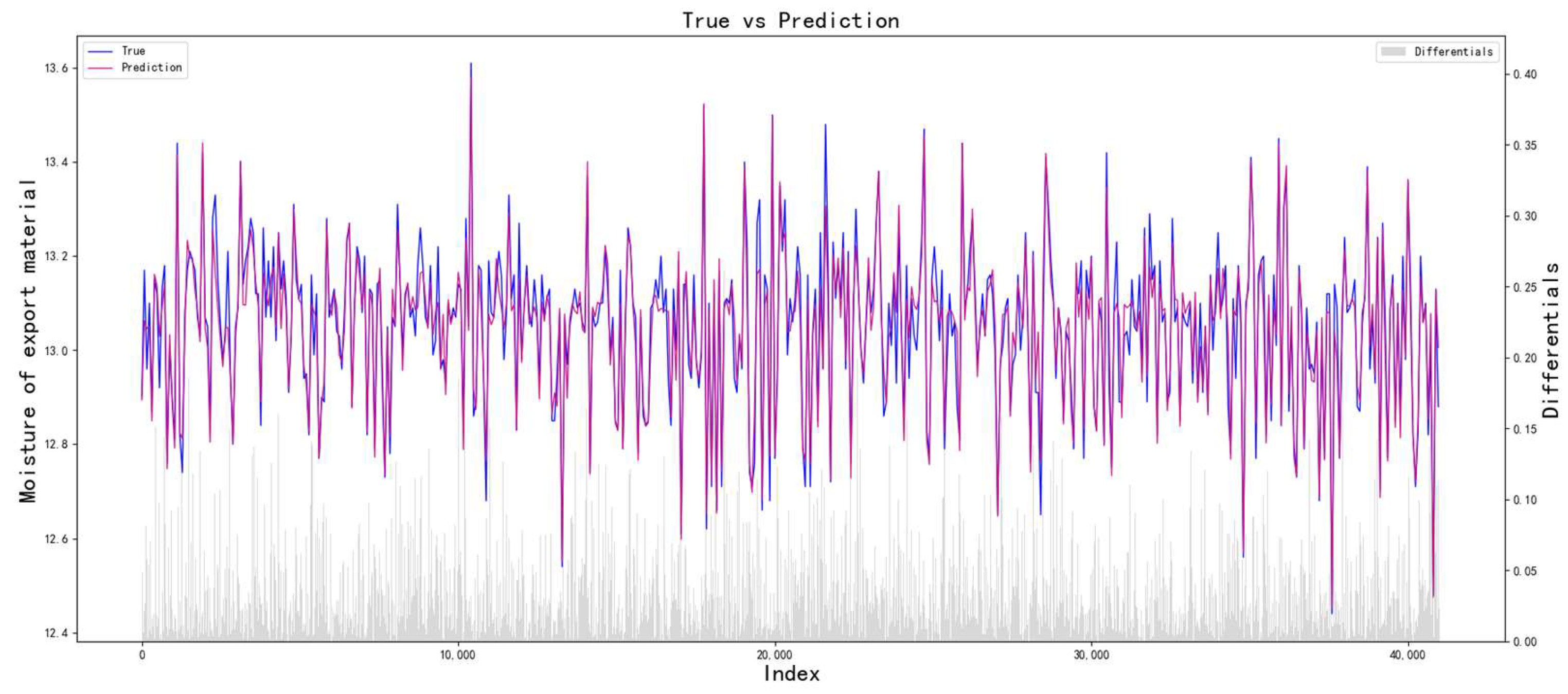
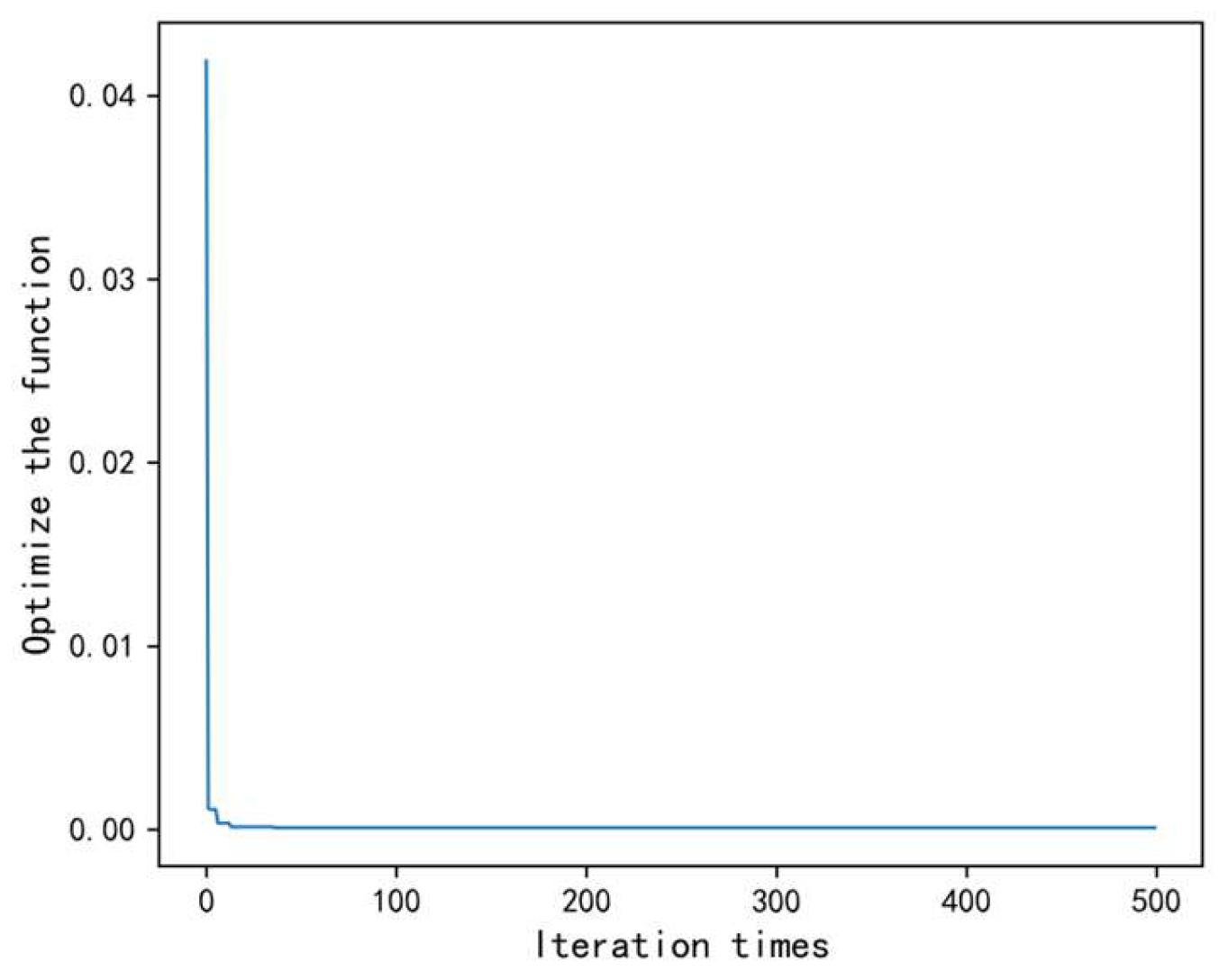
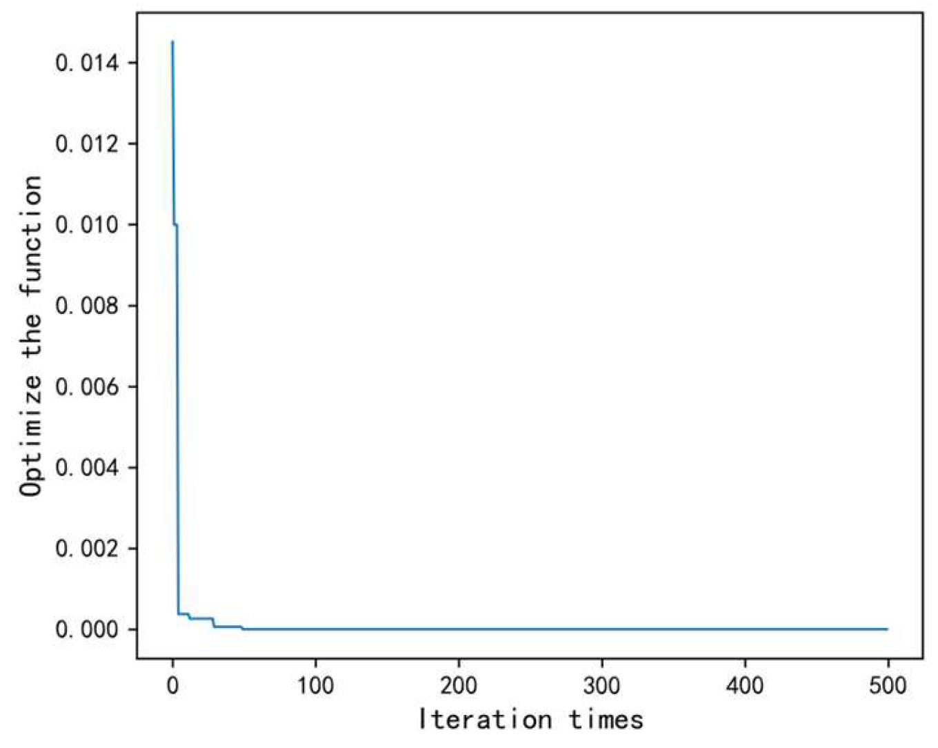
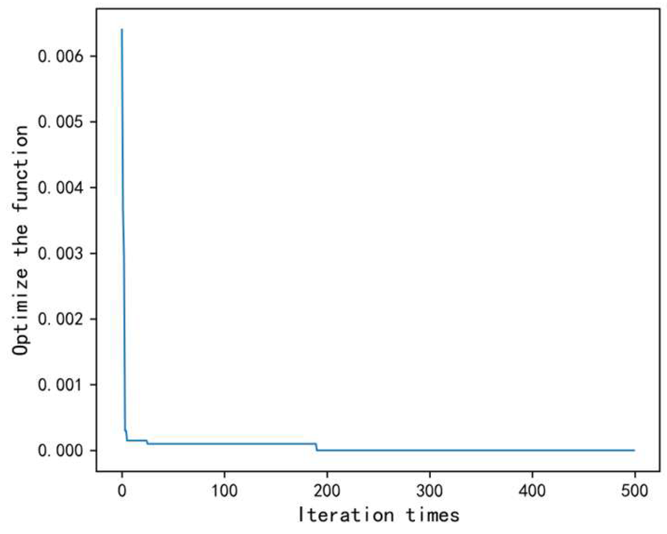
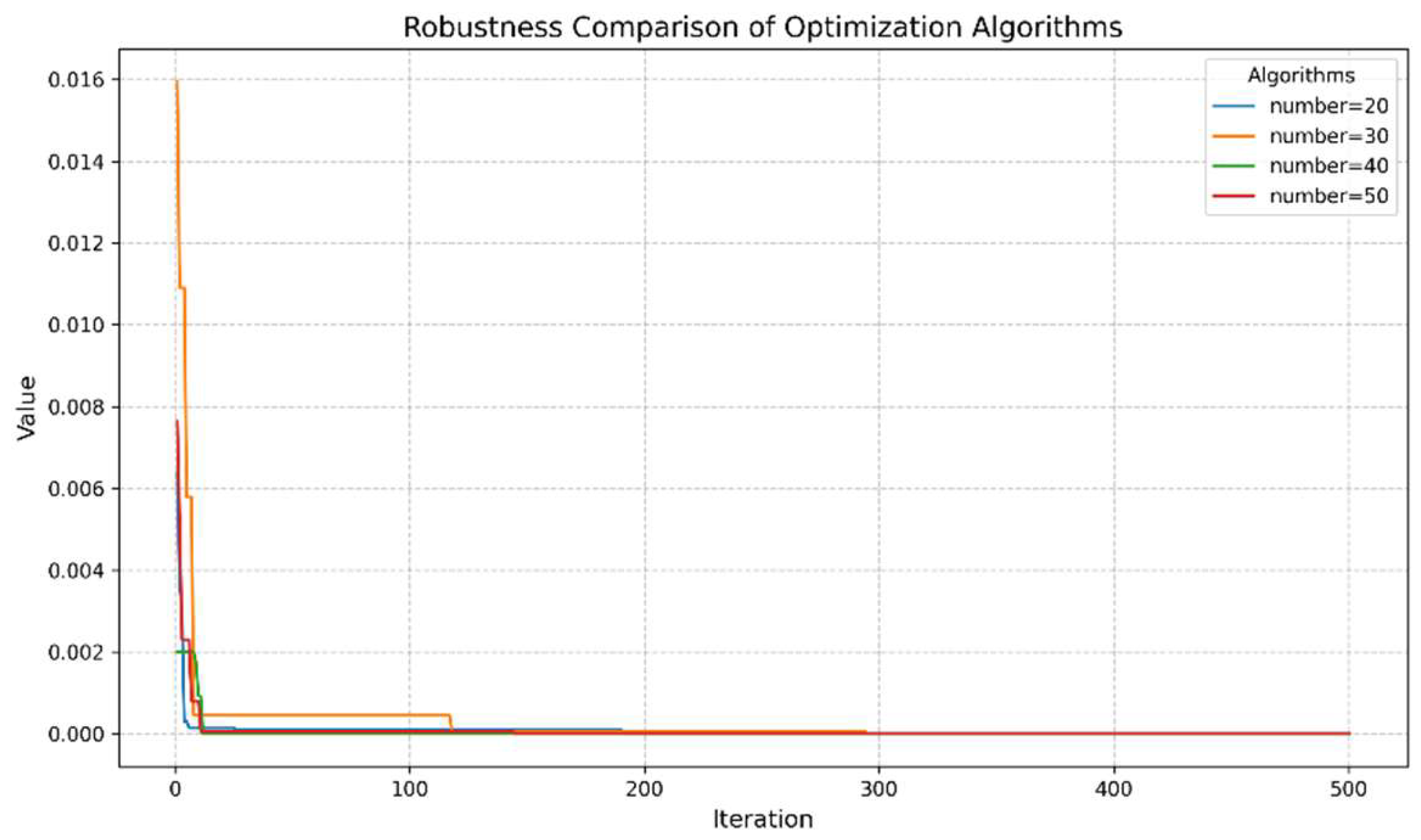
Therefore, according to the above analysis of process parameter optimization and particle swarm optimization algorithm, this paper constructs a multi-level progressive optimization model of process parameters based on an improved particle swarm optimization algorithm. The process of the multi-level progressive optimization model is shown in Figure 3. The model uses a multi-level progressive modeling strategy to establish a nonlinear mapping relationship between process parameters and quality indicators layer by layer and uses the improved particle swarm optimization to search for the optimal combination of process parameters. When constructing the prediction model, the optimal parameter combination of each layer is transmitted to the next layer as a constant input to achieve multi-level progressive optimization of process parameters.

The parameters involved in the algorithm are shown in

Table 1. The algorithm involves parameters.

Serial Number	Parameter	Implication	Serial Number	Parameter	Implication
1	t	Current number of iterations	8	$c_2^{\left(t\right)}$	Acceleration factor 2
2	T	Maximum number of iterations	9	v	Particle velocity
3	fitness	Particle fitness	10	h	Particle position
4	pbest_score	Individual optimal fitness	11	pbest	The best position of individual
5	gbest_score	Global optimal fitness	12	gbest	Global best position
6	${\omega }^{\left(t\right)}$	Inertia weight	13	$r_1$	A random number between $\left[\mathrm{0,1}\right]$
7	$c_1^{\left(t\right)}$	Acceleration factor 1	14	$r_2$	A random number between $\left[\mathrm{0,1}\right]$

.

The process of the multi-level progressive optimization model is as follows:

(1) Randomly initialize the particle swarm.

(2) Calculate the fitness of each particle.

(3) Update pbest and gbest. Each particle searches for the position with the best fitness value as its individual optimal position (pbest), while the position of the particle with the best fitness value across the entire swarm is designated as the global optimal position (gbest).

(4) Update the inertia weight $\omega$ according to Formula (20), and update the acceleration factors $c_1$ and $c_2$ according to Formulas (21) and (22).

(5) Update the particle velocity $v$ and position $h$ according to the formulas.

$$v_i^{t+1}={\omega }^{\left(t\right)}\times v_i^t+c_1^{\left(t\right)}\times r_1\times \left({pbest}_i-h_i^t\right)+c_2^{\left(t\right)}\times r_2\times \left({gbest}_i-h_i^t\right)$$

(24)

$$h_i^{t+1}=h_i^t+v_i^{t+1}$$

(25)

(6) Limit the particle position. According to Formula (23), if any particles are beyond the range, then put them back into the search range.

(7) Determine whether the maximum number of iterations $W$ is reached. If the maximum number of iterations is reached, the optimal process parameters of the layer are recorded. If the maximum number of iterations is not reached, steps (2) to (7) are repeated.

(8) Determine whether the upper limit of the number of groups is reached. If the upper limit of the number is reached, the overall optimal process parameters are output. If the upper limit of the number is not reached, another hierarchical group is added. Based on the optimization of the process parameters of all the previous layers, the prediction model is constructed for the layer, and then steps (2) to (8) are repeated.

Through the above optimization process, the optimal process parameters can be obtained layer by layer, and the optimal process parameters of each layer are based on the optimization of the previous layers. Specifically, this process fully considers the influence of parameters on quality indicators and also greatly weakens the errors caused by non-critical parameters.

3. Experimental Environment and Data Analysis

3.1. Experimental Environment

In order to verify the effectiveness and feasibility of the proposed method, this paper takes the thin plate drying process of a process manufacturing enterprise as the experimental object and carries out multi-level progressive optimization of process parameters. The operating environment of the experiment is shown in

Table 2. Experimental environment.

Hardware Environment		Software Environment
Name	Equipment Model	Name	Version
Processor	Intel 12th Generation Core i5-12600KF	Python	3.6
Graphics card	NVIDIA GeForce RTX 4060 Ti	Pycharm	2022.1.4
Running memory	32 GB	Scikit-learn	0.24.1
Operating system	Win11 Home China 23H2 64-bit	Joblib	1.0.1

:

The selection of hyperparameters is crucial to the performance and stability of the model. Reasonable hyperparameter settings can effectively improve the training efficiency, accuracy, and generalization ability of the model. Especially in the optimization problem of high-dimensional parameters, the appropriate hyperparameter configuration can help the model find the optimal solution in the complex parameter space, thereby improving the performance of the model. Therefore, the super parameter values shown in

Table 3. Super parameter setting.

Hyperparameter Name	Values	Hyperparameter Name	Values
n_estimators	200	${\omega }_{\mathrm{m}\mathrm{i}\mathrm{n}}$	0.2
max_depth	18	$c_{1max}$	2
swarm_size	20	$c_{1min}$	1
max_iter	500	$c_{2max}$	2
${\omega }_{max}$	0.9	$c_{2min}$	1

are used in the modeling and optimization process. On this basis, in order to further prevent overfitting and improve the stability of the model, this paper introduces the dropout layer in the training process.

3.2. Experimental Data

This study takes the thin plate drying process of a process production line as an example. The basic process of this process is as follows: the raw material reaches the drum from the front chamber inlet and rolls to the rear chamber outlet under the rotation of the inclined installed drum. The pressurized steam is sent all the way to the heat exchange device in the drum through the rotating joint. The heat exchange device is a thin plate structure. On the one hand, it heats the material, and on the other hand, it plays the role of transporting raw materials so that the material rolls up and down. The pressurized steam enters another way into the heat exchanger controlled by the electric angle stroke actuator, and the hot air makes the material suspend and roll evenly heated. The temperature and flow of hot air, the steam pressure of the heat exchange device, and the rotation speed of the drum will lead to the change in the moisture content of the material. The moisture, miscellaneous gas, and dust evaporated from the material are discharged through the dust removal system with hot air as the carrier, as shown in Figure 4.

In this study, the process data are collected in real time by the sensors deployed in the equipment terminal of the production line, and each sensor records the process parameters regularly every second. The collected real-time data are connected to the MES system (production management system) through the sensor and automatically uploaded to the system for storage and processing in chronological order to form a complete process data set. In order to verify and evaluate the effectiveness of the proposed method, this study exported the process data of October 2022 from the MES system of the production line for analysis, and the specific data information is shown in

Table 4. Experimental data.

Index	Batch Number	Acquisition Time	Exhaust Wind Temperature	Exhaust Moisture Humidity	Inlet Material Temperature
1	YZ122101706	18 October 2022 10:17:27	97.979065	6.158636	33.383970
2	YZ122101706	18 October 2022 10:17:28	97.852715	6.274606	32.548466
3	YZ122101706	18 October 2022 10:17:29	97.852715	6.274606	32.939090
4	YZ122101706	18 October 2022 10:17:30	97.693410	6.259346	33.072914
……	……	……	……	……	……
205,036	YZ122102601	26 October 2022 14:27:23	76.961580	9.033479	41.532840

. According to the data table, the collected records include process parameters such as ‘batch number’, ‘collection time’, ‘exhaust air temperature’, ‘exhaust air humidity’, and ‘inlet material temperature’, totaling 205,036 records.

The specific analysis of the process data of the drying process shows that the process data contains 26 process parameters and 1 quality index, and most of the process parameter names are lengthy. In order to facilitate the subsequent analysis and representation, the process data set is re-encoded, as shown in

Table 5. Process parameter numbering.

Code	Name of Process Parameters	Code	Name of Process Parameters
$X_1$	Input Material Moisture	$X_{15}$	Actual Mixed Air Gate
$X_2$	Input Material Flow	$X_{16}$	Hot Air Fan Frequency
$X_3$	Input Material Temperature	$X_{17}$	HT Steam Pressure
$X_4$	Dehumidifying Wind Temperature	$X_{18}$	HT Steam Inflow
$X_5$	Dehumidifying Wind Humidity	$X_{19}$	Thin Plate Steam Temperature
$X_6$	Dehumidifying Wind Speed	$X_{20}$	Thin Plate Steam Pressure
$X_7$	Dehumidifying Wind Volume	$X_{21}$	Cylinder Wall Temperature Average
$X_8$	Dehumidifying Wind Gate Opening	$X_{22}$	Cylinder Wall Temperature Pressure Conversion
$X_9$	Dehumidifying Negative Pressure	$X_{23}$	Thin Plate Condensate Temperature
$X_{10}$	Actual Drum Rotation Speed	$X_{24}$	Cylinder Wall Temperature (Front)
$X_{11}$	Main Drive Motor Actual Value	$X_{25}$	Cylinder Wall Temperature (Middle)
$X_{12}$	Actual Hot Air Temperature	$X_{26}$	Cylinder Wall Temperature (Rear)
$X_{13}$	Front Room Hot Air Duct Wind Speed	$Y$	Output Material Moisture
$X_{14}$	Front Room Hot Air Duct Wind Volume

. In the process of data acquisition, due to improper operation, sensor failure, downtime, or material shortage, the collected data often contains null values and outliers. In order to improve the accuracy of process modeling and prediction, the average filling method is used to fill the missing data to ensure the integrity of the data, and then the $3\sigma$ method is used to filter and remove the data so as to improve the accuracy and stability of the subsequent analysis.

4. Results and Discussion

4.1. Multi-Level Progressive Parameter Optimization Analysis

(1)

Parameter importance assessment

Through analysis, it is found that the influence of different process parameters on quality indicators is different. In order to further reveal this phenomenon, this paper calculates the correlation between process parameters and quality indicators through correlation analysis. The results are shown in

Table 6. Correlation degree of process parameters.

Parameter Code	Correlation	Parameter Code	Correlation	Parameter Code	Correlation
$X_1$	0.663993	$X_{10}$	0.406856	$X_{19}$	0.697866
$X_2$	0.620857	$X_{11}$	0.406891	$X_{20}$	0.822104
$X_3$	0.648222	$X_{12}$	0.428172	$X_{21}$	0.898596
$X_4$	0.133950	$X_{13}$	0.421117	$X_{22}$	0.825326
$X_5$	0.935450	$X_{14}$	0.421119	$X_{23}$	0.737293
$X_6$	0.839090	$X_{15}$	0.252147	$X_{24}$	0.904791
$X_7$	0.839090	$X_{16}$	0.451571	$X_{25}$	0.882176
$X_8$	0.834964	$X_{17}$	0.469450	$X_{26}$	0.882143
$X_9$	0.663993	$X_{18}$	0.474279

.

According to the above table, it can be proved that the influence of different process parameters on quality indicators is different. Therefore, when the process parameters are stratified, they should be divided based on their relative influence on quality indicators. The parameters with greater influence should be classified into the key level, and those with less influence should be classified into the secondary level. When the quality fluctuates, the product quality can be quickly controlled and optimized by adjusting the parameters of the key levels. Adjusting the parameters of the secondary level helps to reduce errors in quality control. By comprehensively adjusting the process parameters of each level, the precise control of quality indicators can be achieved. Therefore, the correlation degree ranking of process parameters is very important for hierarchical optimization, and the rank results are shown in

Table 7. Correlation ranking.

Serial Number	Parameter Code	Serial Number	Parameter Code	Serial Number	Parameter Code
1	$X_5$	10	$X_{20}$	19	$X_{16}$
2	$X_{24}$	11	$X_9$	20	$X_{12}$
3	$X_{21}$	12	$X_{23}$	21	$X_{14}$
4	$X_{25}$	13	$X_{19}$	22	$X_{13}$
5	$X_{26}$	14	$X_1$	23	$X_{11}$
6	$X_6$	15	$X_3$	24	$X_{10}$
7	$X_7$	16	$X_2$	25	$X_{15}$
8	$X_8$	17	$X_{18}$	26	$X_4$
9	$X_{22}$	18	$X_{17}$

.

(2)

Hierarchical division of parameters

In order to more accurately stratify the sorted process parameters, the random forest regression model is used to evaluate the contribution of each process parameter to the quality index so as to realize the hierarchical division of process parameters. The first round of the hierarchical division process is shown in Figure 5.

It can be seen from Figure 5 that when the number of process parameters reaches 6, the $R^2$ change rate value is almost below 0.003. Although the number of process parameters is greater than 6, $R^2$ increases with the increase in process parameters, but its growth rate is very low, and the corresponding value $R^2$ is 0.8349 when the number of parameters reaches 6, indicating that these six parameters have a relatively strong ability to explain quality indicators. On this basis, observing the comprehensive index value of Figure 5, it can be found that with the increase in parameters, when the number of parameters reaches 6, the value of the comprehensive index is 0.000503, and it is less than 0.003 for the first time. Since then, all the comprehensive index values have been kept within the range of 0.003, indicating that the accuracy of the model has stabilized. Based on this, it can be considered that the model shows high stability at this time, and the explanatory power is sufficient when the number of parameters is 6. Therefore, these six process parameters are divided into one layer. Next, these six process parameters are eliminated, and the remaining parameters are divided into levels based on their contribution to the quality indicators. The second round of the hierarchical division process is shown in Figure 6.

Similarly, it can be seen from Figure 6 that when the number of process parameters reaches 12, the $R^2$ change rate value is almost below 0.003, and the corresponding $R^2$ value is 0.8828, indicating that the parameter combination has high explanatory power for quality indicators. At the same time, by observing the comprehensive index value, it can be found that although the comprehensive index is less than 0.003 for the first time at the 8th parameter, the value of the comprehensive index has not been kept below 0.003 since then, so this point is skipped. When the number of parameters is close to 12, the value of the comprehensive index is less than 0.003 again; the value is 0.002810, and all the subsequent comprehensive index values remain in a very small fluctuation range, indicating that the accuracy of the model has stabilized. It shows that the model has stabilized under this parameter combination. Therefore, the 12 process parameters are divided into one layer. Next, these 12 process parameters are eliminated, and the remaining parameters are hierarchically divided. The third round of the hierarchical division process is shown in Figure 7.

According to the results of the third round of the process parameter stratification process, it can be seen that with the increase in process parameters, the change rate of $R^2$ did not show a clear regularity and failed to stabilize. At the same time, the maximum value of $R^2$ is only 0.6025, indicating that the eight parameters have relatively weak explanatory power for quality indicators, and the comprehensive index value does not show a stable trend. In addition, from the ranking results of correlation degree, the correlation degree of these 8 parameters is lower than 0.5. Therefore, this study believes that it is not necessary to further stratify these eight parameters and directly classify them into the same layer. The final hierarchical division results are shown in

Table 8. The results of the hierarchical division of parameters.

Hierarchy	Parameter Code		Hierarchy	Parameter Code
First Level	$X_5$	$X_{25}$	Second Level	$X_7$	$X_1$
	$X_{24}$	$X_{26}$		$X_8$	$X_3$
	$X_{21}$	$X_6$		$X_{22}$	$X_2$
Third Level	$X_{16}$	$X_{11}$		$X_{20}$	$X_{18}$
	$X_{12}$	$X_{10}$		$X_9$	$X_{17}$
	$X_{14}$	$X_{15}$		$X_{23}$
	$X_{13}$	$X_4$		$X_{19}$

.

Therefore, this paper divides the various process parameters into layers according to the importance of the relative quality indicators. The first layer is the key parameter combination, and the number of parameters is 6. The second layer is the sub-important parameter combination; the number of parameters is 12, and the third group is the redundant parameter combination; the number of parameters is 8.

(3)

Progressive optimization layer by layer

In order to avoid the influence of redundant parameters on the optimization accuracy of key parameters, this paper will first optimize the redundant parameters of the third layer. Then, on the basis of determining 8 optimal redundant parameters, the 12 sub-important parameters of the second layer are optimized. Finally, on the basis of the second and third layers optimization, the key parameters are optimized to obtain more accurate optimization results. Among them, the process flow data of each layer are divided into the training set and test set according to the ratio of 8:2, and the quality index prediction model is established based on the training set. At the same time, the improved particle swarm optimization is introduced to optimize the process parameters. The prediction results of the third layer of quality indicators are shown in Figure 8.

After comparing and analyzing the true value and predicted value of the moisture content of the export material, it was found that the $MAE$ of the third layer was 0.0817, $RMSE$ was 0.1137, and $R^2$ was 0.6022. In general, the prediction accuracy of the model in this layer is low, which further verifies the rationality of dividing these parameters into redundant parameter combinations. On this basis, the improved particle swarm optimization is used to search the optimal parameter combination of the third layer, whose fitness curve is shown in Figure 9.

It can be seen from the results that on the data set of the third layer of process parameter combination, the fitness tends to be stable after 31 rounds of iteration, ranging from 0 to 0.0001. At this time, the selected parameter combination minimizes the prediction error at this level. The optimization results of this layer are shown in

Table 9. The third layer of optimal process parameters.

Parameter Code	Optimal Value	Parameter Code	Optimal Value	Parameter Code	Optimal Value
$X_{16}$	17.9962	$X_{13}$	3.8067	$X_{15}$	49.1706
$X_{12}$	113.2850	$X_{11}$	32.3517	$X_4$	89.6226
$X_{14}$	705.1345	$X_{10}$	11.0000

.

Since the third layer of process parameters is a combination of redundant parameters, directly retaining these parameters will lead to redundancy in the parameter optimization process, and removing them would lead to certain errors in the optimization results. Therefore, the process parameters of this level are optimized and analyzed separately, and then the optimal combination of these process parameters is output as a constant to the prediction model of the second layer, and the steps of establishing the prediction model and improving the particle swarm optimization algorithm in the third layer are repeated. The prediction results of the second layer quality index are shown in Figure 10.

After comparing and analyzing the true value and predicted value of the moisture content of the export material, it was found that the $MAE$ of the second layer was 0.0446, $RMSE$ was 0.0604, and $R^2$ was 0.8878. Then, the improved particle swarm optimization is used to search for the optimal parameter combination of the second layer. The fitness curve of the optimization process is shown in Figure 11.

It can be seen from the results that on the basis of the combination optimization of process parameters in the third layer, the fitness in this layer tends to be stable after 86 rounds of iteration, ranging from 0 to 0.0001. At this time, the selected parameter combination minimizes the prediction error at this level. The optimization results of this layer are shown in

Table 10. The second layer of optimal process parameters.

Parameter Code	Optimal Value	Parameter Code	Optimal Value	Parameter Code	Optimal Value
$X_7$	1178.3582	$X_9$	−7.8251	$X_3$	50.9124
$X_8$	31.8496	$X_{23}$	97.0625	$X_2$	1002.6129
$X_{22}$	121.2238	$X_{19}$	112.7577	$X_{18}$	47.3938
$X_{20}$	0.1338	$X_1$	7.3400	$X_{17}$	0.2354

.

The optimal combination of process parameters corresponding to the second and third layers is output as a constant to the prediction model of the first layer, and then the steps of establishing the prediction model and improving the particle swarm optimization of the above two layers are repeated. The results are shown in Figure 12.

Similarly, by comparing and analyzing the actual value and predicted value of the moisture content of the export material, it can be found that on the basis of the optimization of the second and third layers process parameters, the $MAE$ of the first layer was 0.0352, $RMSE$ was 0.0487, and $R^2$ was 0.9271. In order to find the optimal combination of the first layer of process parameters, the improved particle swarm optimization was used to search for the optimal parameter combination of the first layer. The fitness curve of the optimization process is shown in Figure 13.

It can be seen from the results that on the basis of the optimization of the second and third layers process parameters, the fitness of the particle swarm optimization algorithm in this layer tends to be stable after 37 rounds of iteration, ranging from 0 to 0.0001. At this time, the optimization results of this layer are shown in

Table 11. The first layer of optimal process parameters.

Parameter Code	Optimal Value	Parameter Code	Optimal Value	Parameter Code	Optimal Value
$X_5$	17.2189	$X_{21}$	112.5879	$X_{26}$	113.2992
$X_{24}$	110.7978	$X_{25}$	110.2643	$X_6$	5.9632

.

In this paper, the optimal values of all process parameters are determined by the layer-by-layer progressive optimization method. In practical operation, according to the optimized parameter setting, the $R^2$ of the model reaches 0.9271, and the corresponding quality index prediction value is 12.99. The results show that the quality indicators predicted by this method are closer to the ideal value set by the enterprise in the quality management rules, which proves the effectiveness of the proposed method.

4.2. Comparison Validation

In order to verify the feasibility and effectiveness of the proposed method, this paper uses two optimization strategies for comparative analysis: extraction of key parameters optimization and overall optimization. Firstly, the corresponding data sets are used to train the prediction model respectively, and its performance is verified on the test set. On this basis, combined with the improved particle swarm optimization algorithm, the optimal parameter combination is searched. Finally, by comparing the performance of these two process parameter optimization methods and the multi-level progressive optimization method in predicting performance and optimization results, the feasibility and effectiveness of the proposed method in practical application are verified.

(1)

Analysis of optimization method for extracting key parameters

When the optimization method of extracting key parameters is used, this paper divides the corresponding process parameter data set into the training set and test set according to the ratio of 8:2 and constructs the quality indicators prediction model based on the training set. In order to further optimize the process parameters, the improved particle swarm optimization algorithm is introduced to search for the optimal parameter combination. This method reduces the complexity of parameter optimization by focusing on the most influential key parameters, with a $R^2$ of 0.8515 and a predicted quality index of 12.96. This method effectively reduces the complexity of the model by extracting key parameters. Among them, the fitness convergence curve of this method is shown in Figure 14.

The above diagram shows the fitness convergence curve when using the improved particle swarm optimization algorithm for parameter optimization. After 50 rounds of iteration, the fitness value tends to be stable, and the fluctuation range is between 0 and 0.0001. It can be seen that in the case of focusing on key parameters, the algorithm converges faster and accelerates the search process of the optimal solution. This shows that the method effectively reduces the complexity of the model and accelerates the search process for the optimal solution by focusing on the most influential key parameters. The comparative experimental analysis of this optimization method and the multi-level progressive optimization is shown in

Table 12. The comparison results of key parameter optimization and multi-level progressive optimization are extracted.

Type	Parameter Number	Number of Optimizations	$\mathit{M}\mathit{A}\mathit{E}$	$\mathit{R}\mathit{M}\mathit{S}\mathit{E}$	${\mathit{R}}^{\mathbf{2}}$	Iteration Times	Run Time	Optimize Accuracy
Extract key parameters	6	6	0.050028	0.069450	0.851507	50	90	99.69%
Multi-level progression	8 + 12 + 6	6	0.035219	0.048677	0.927054	37	55	99.92%

. Among them, in order to ensure a reasonable comparison with the optimization method of extracting key parameters, this paper assumes that the non-key layer parameters have been optimized and input as constants into the optimization process of the key layer to ensure the consistency of the two methods in the number of optimized parameters.

It can be seen from the comparison results that the quality index prediction value of the multi-level progressive optimization method in the optimization process is better fitted around 12.99. That is, more prediction values are close to the ideal value. The predicted value of the quality index corresponding to the optimization method of extracting the key parameters is better fitted near 12.96. This shows that the optimization accuracy of multi-level progressive optimization is higher, and the predicted quality indicators are closer to the ideal value in the quality management rules of the enterprise. Although the optimization efficiency of this method is not much different from that of the extraction of key parameters, it is obviously superior to the latter in terms of optimization accuracy. This difference is mainly because the optimization method of extracting key parameters only considers the key parameters and does not fully analyze the influence of other parameters on the quality index, while the multi-level progressive optimization systematically analyzes the interaction between all parameters so as to obtain more accurate optimization results.

(2)

Analysis of the overall optimization method

Similarly, when using the overall optimization method, this paper divides the process parameter data into the training set and test set according to the ratio of 8:2 and constructs the quality indicators prediction model based on the training set. Then, the improved particle swarm optimization algorithm is introduced to search for the optimal parameter combination. This method effectively improves the prediction accuracy of process parameters by paying attention to the comprehensive influence of the overall process parameters. The $R^2$ value reaches 0.927059, and the predicted quality index is 13.05. Among them, the fitness convergence curve of this method is shown in Figure 15.

In the optimization process of the improved particle swarm optimization, after 301 rounds of iteration, the fitness value tends to be stable, and the fluctuation range is between 0 and 0.0001. This shows that the method fully considers the influence of all process parameters, resulting in a significant decrease in optimization efficiency. The comparative experimental analysis of the overall prediction optimization method and the multi-level progressive optimization is shown in

Table 13. The comparison results of overall optimization and multi-level progressive optimization.

Type	Parameter Number	Number of Optimizations	$\mathit{M}\mathit{A}\mathit{E}$	$\mathit{R}\mathit{M}\mathit{S}\mathit{E}$	${\mathit{R}}^{\mathbf{2}}$	Iteration Times	Run Time	Optimize Accuracy
Overall optimization	26	26	0.035219	0.048675	0.927059	301	576	99.62%
Multi-level progression	8 + 12 + 6	8 + 12 + 6	0.035219	0.048677	0.927054	154	213	99.92%

.

It can be seen from the results that the predicted value of the quality index corresponding to the overall optimization method is better fitted near 13.05. This shows that the optimization accuracy of multi-level progressive optimization is higher, and the predicted quality indicators are closer to the ideal values set in the quality management rules of the enterprise. Although the accuracy of multi-level progressive optimization is not much different from that of the overall optimization, its computational efficiency is significantly improved, and the number of iterations and running time are increased by 49% and 63%, respectively, showing stronger application potential.

By comparing and analyzing the results of the proposed method and the other two optimization methods, it can be seen that the multi-level progressive optimization is significantly better than the overall optimization in terms of operating efficiency, which not only reduces the number of iterations but also shortens the running time. At the same time, compared with the optimization of extracting key parameters, multi-level progressive optimization overcomes the limitation of focusing only on key parameters while improving the optimization accuracy and can more comprehensively consider the interaction between parameters, thus effectively dealing with the complexity of parameter optimization in the process industry. Therefore, multi-level progressive optimization shows higher potential in practical applications and provides an effective solution to balance optimization efficiency and accuracy.

(3)

The comparison and analysis of optimization algorithms

In order to verify the effectiveness of the IPSO algorithm, it is further compared with the conventional PSO, genetic algorithm (GA), and differential evolution algorithm (DE), and also compared with other improved algorithms proposed in the existing literature [32,33]. All algorithms run under the same experimental environment and parameter settings, and the comparison results are shown in Table 14.

Table 14. Comparison results of optimization algorithms.

Optimistic Algorithm	Adaptation Degree
PSO	$3.55\times {10}^{-15}$
DE	$1.24\times {10}^{-14}$
GA	0.00015
IMPA [32]	$1.07\times {10}^{-14}$
OPSO [33]	$8.88\times {10}^{-15}$
Ours	$1.78\times {10}^{-15}$

Table 14. Comparison results of optimization algorithms.

Optimistic Algorithm	Adaptation Degree
PSO	$3.55\times {10}^{-15}$
DE	$1.24\times {10}^{-14}$
GA	0.00015
IMPA [32]	$1.07\times {10}^{-14}$
OPSO [33]	$8.88\times {10}^{-15}$
Ours	$1.78\times {10}^{-15}$

From the results, it can be seen that the IPSO algorithm has a significant improvement in accuracy compared with conventional algorithms such as PSO, GA, and DE, as well as other improved algorithms proposed in literature [32,33], and its accuracy is increased by an average of 79.81%. This result shows that although the number of iterations of the IPSO algorithm increases slightly, it performs better in solving local convergence problems. Therefore, IPSO significantly enhances the search ability of particles when approaching the optimal solution by introducing strategies such as decreasing inertia weight, adaptive change of acceleration factor, and particle position constraint so as to achieve better accuracy than all comparison algorithms.

In order to verify the robustness of the proposed IPSO algorithm, experiments are carried out under different initial population configurations. The experimental results are shown in Figure 16.

It can be seen from the results that although different initial population configurations are set, the convergence accuracy obtained is not much different. The convergence fluctuation range of the four groups of experiments is between 0 and 0.0001, which shows that the IPSO algorithm proposed in this paper has strong robustness and can maintain stable optimization performance under different initial conditions.

In summary, these experimental results prove that the proposed method not only has good applicability and reliability but also can maintain superior optimization performance under different conditions, further consolidating its effectiveness in practical applications.

(4)

Comparative analysis of importance assessment methods

In order to systematically evaluate the influence of the change of parameter importance ranking on multi-level progressive optimization, this study adopts two different parameter importance evaluation methods: XGBoost and the Spearman rank correlation evaluation method. These two methods are used to evaluate the relative importance of each process parameter to the process quality and prepare for the subsequent multi-level progressive optimization according to different ranking results. All experiments were carried out in the same model setting and experimental environment to ensure the comparability of the results. Firstly, the XGBoost method is used to rank the importance of process parameters. As a tree model based on gradient lifting, this method can effectively process high-dimensional data and provide accurate ranking results. Subsequently, the Spearman rank correlation method was used to rank the process parameters. This method evaluates the influence of the parameters on the process quality by calculating the rank correlation between the parameters. Among them, the results of the two groups of methods are shown in

Table 15. The comparison results of importance assessment methods.

XGBoost				Spearman Rank Correlation
Serial Number	Parameter Code	Serial Number	Parameter Code	Serial Number	Parameter Code	Serial Number	Parameter Code
1	$X_{23}$	14	$X_{20}$	1	$X_5$	14	$X_{18}$
2	$X_9$	15	$X_{18}$	2	$X_{23}$	15	$X_4$
3	$X_{12}$	16	$X_5$	3	$X_{20}$	16	$X_9$
4	$X_{26}$	17	$X_2$	4	$X_{22}$	17	$X_{17}$
5	$X_{21}$	18	$X_6$	5	$X_{19}$	18	$X_{13}$
6	$X_{17}$	19	$X_8$	6	$X_{12}$	19	$X_{14}$
7	$X_4$	20	$X_3$	7	$X_{21}$	20	$X_3$
8	$X_{15}$	21	$X_{13}$	8	$X_{24}$	21	$X_8$
9	$X_{25}$	22	$X_7$	9	$X_{25}$	22	$X_1$
10	$X_{24}$	23	$X_{16}$	10	$X_{26}$	23	$X_{15}$
11	$X_{19}$	24	$X_{11}$	11	$X_2$	24	$X_{10}$
12	$X_1$	25	$X_{10}$	12	$X_6$	25	$X_{11}$
13	$X_{22}$	26	$X_{14}$	13	$X_7$	26	$X_{16}$

.

Based on the above two sorting results, the hierarchical method proposed in this paper is used to stratify, which provides support for the subsequent multi-level progressive prediction optimization. The stratification results of the two groups of sorting methods are shown in

Table 16. The results of the hierarchical division of parameters.

XGBoost		Spearman Rank Correlation
Hierarchy	Parameter Code	Hierarchy	Parameter Code
First Level	$X_{23}$, $X_9$, $X_{12}$, $X_{26}$, $X_{21}$, $X_{17}$	First Level	$X_5$, $X_{23}$, $X_{20}$, $X_{22}$, $X_{19}$, $X_{12}$, $X_{21}$, $X_{24}$
Second Level	$X_4$, $X_{15}$, $X_{25}$, $X_{24}$, $X_{19}$, $X_1$, $X_{22}$, $X_{20}$, $X_{18}$, $X_5$, $X_2, X_6$	Second Level	$X_{25}$, $X_{26}$, $X_2$, $X_6$, $X_7$, $X_{18}$, $X_4$, $X_9$
Third Level	$X_8$, $X_3$, $X_{13}$, $X_7$, $X_{16}$, $X_{11}$, $X_{10}$, $X_{14}$	Third Level	$X_{17}$, $X_{13}$, $X_{14}$, $X_3$, $X_8$, $X_1$, $X_{15}$, $X_{10}$, $X_{11}$, $X_{16}$

.

In order to further compare the influence of different importance assessment methods on the prediction accuracy of multi-level progressive modeling, this study uses these two methods to optimize multi-level progressive prediction on the basis of the above stratification. The results are shown in

Table 17. The comparison results of different importance assessment methods.

Importance Assessment Method	$\mathit{M}\mathit{A}\mathit{E}$	$\mathit{R}\mathit{M}\mathit{S}\mathit{E}$	${\mathit{R}}^{\mathbf{2}}$
Spearman Rank Correlation	0.037089	0.050803	0.920540
XGBoost	0.035223	0.048687	0.927024
Ours	0.035219	0.048677	0.927054

. The table shows the comparison results of multi-level progressive modeling prediction accuracy obtained by these two methods and intuitively compares the prediction effects of different sorting methods after optimization.

It can be seen from the experimental results that the final prediction accuracy will also be significantly affected when different importance evaluation methods are used to lead to changes in the order of parameter importance. This is because different evaluation methods have differences in measuring the correlation of parameters, which leads to different ranking results, and the ranking results directly determine the parameter grouping structure in hierarchical optimization. Further experiments show that the method of sorting the importance of parameters by Pearson correlation analysis shows the best effect in optimizing stratification. This result further verifies the rationality and necessity of the proposed method in optimizing hierarchical grouping.

5. Conclusions and Future Research

Aiming at the challenges of computational complexity caused by high-dimensional parameters in complex process industries, this paper proposes a multi-level progressive parameter optimization method for complex process industries, which realizes the efficient prediction and optimization of complex process parameters. The main conclusions are as follows: In this paper, based on the importance evaluation of process parameters, the importance ranking of process parameters is completed, and the parameter levels are reasonably divided by combining the comprehensive evaluation indexes such as model stability. Then, combined with the parameter transfer mechanism and the improved particle swarm optimization, a multi-level progressive process parameter optimization method is proposed. This method effectively avoids the risk of missing other important parameters in the method of extracting key parameters and significantly reduces the computational complexity of high-dimensional optimization problems through a multi-level parameter transfer mechanism. Compared with the existing optimization methods, the multi-level progressive optimization method proposed in this paper achieves an excellent balance between optimization accuracy and computational complexity, which not only ensures higher optimization accuracy but also significantly reduces the computational burden.

In summary, the multi-level progressive parameter optimization method for the complex process industry proposed in this paper successfully solves the complexity problem of parameter optimization in the complex process industry and shows significant optimization efficiency and accuracy. This method has broad application potential in practical applications and provides an innovative solution for parameter optimization problems in complex process industries. However, considering the application of real-time or large-scale industrial systems, the scalability of the method still needs further study. In response to the challenges of large-scale data processing and real-time optimization, future research will focus on the adaptability and efficiency improvement of this method in high-dimensional, real-time systems. In addition, the further optimization of the cross-layer parameter interaction processing mechanism will help to improve the stability and applicability of the overall algorithm. Specifically, the cross-layer interaction framework can establish a collaborative mechanism based on different levels of parameters to enhance the system’s responsiveness in dealing with complex parameter relationships. The framework needs to consider the information transmission, feedback loop, and potential interaction between levels and propose reasonable interaction rules and processing methods. In addition, potential challenges in cross-layer interactions may include conflicts between parameters at different levels, information overload, and the stability of feedback mechanisms. In order to cope with these challenges, future research will focus on solving these problems to ensure the applicability of the model in large-scale and dynamically changing environments. At the same time, for the problem of computational cost, lightweight algorithms and parallel computing technologies can be explored to reduce resource consumption in the optimization process. These improvements will help the method achieve more efficient and accurate optimization in a wider range of industrial applications.