Abstract
Transitional shale gas represents a critical frontier for China’s oil and gas exploration, characterized by extensive distribution and substantial resource potential. However, its frequent interbedding with coal seams and tight sandstones results in a complex reservoir architecture, significantly increasing extraction challenges. Hydraulic fracturing remains the primary method for effectively stimulating production in such reservoirs. Nevertheless, due to the complex stacking patterns of coal, shale, and tight sandstone layers, fracturing often generates complex fracture networks, leading to pronounced stress-sensitive effects and fracture interference during production. Moreover, the development of transitional shale gas reservoirs typically employs multi-well pad fracturing (“factory-mode” drilling) with tight well spacing, intensifying the well interference and its impact on well group productivity. These factors collectively complicate post-fracturing production forecasting. Existing productivity models predominantly focus on single-lithology reservoirs with idealized fracture networks, neglecting critical factors such as the fracture interference, well interference, and stress sensitivity. To address this gap, this study targets the Ordos Basin’s transitional shale gas reservoirs. By integrating the multi-lithology, multi-layer stacked reservoir characteristics, we developed a productivity model for infill wells in such reservoirs. Using a semi-analytical approach, we analyzed post-fracturing production behavior in horizontal wells, optimized key development parameters, and provided a scientific basis for the efficient development of these reservoirs.
1. Introduction
Shale gas has gradually become an important alternative field for unconventional natural gas exploration and development in China [1,2,3]. China has a huge potential for shale gas resources, which can be further classified into three types based on sedimentary environments: marine, marine–continental transitional, and continental. Among them, the geological resources of marine–continental transitional shale gas account for approximately 25% of the total geological resources of shale gas in China [4,5,6]. The scale of mud shale in marine–continental transitional shale reservoirs is smaller compared to marine shale reservoirs, and the single-layer thickness of shale, coal rock, and tight sandstone reservoirs is thin, making their individual development economically unviable. However, shale layers frequently interbed with coal rock, tight sandstone, and other layers, with rich organic matter and a considerable cumulative thickness, resulting in a considerable total resource volume. The combined development of multiple layers has good economic benefits. The multi-stage and multi-segment fracturing of horizontal wells is the main technical means for its development.
Compared with the exploitation period of a single shale gas reservoir, the development time of marine–continental transitional reservoirs at home and abroad is relatively short, and there are few existing marine–continental transitional fractured horizontal wells. There are also few studies by scholars at home and abroad on the marine–continental transitional infill wells. However, the research on shale gas reservoir fractured horizontal well groups, especially infill adjustment wells, is indeed extensive. After long-term practice and exploration, a relatively complete shale gas development system has been formed, namely the development technology of “horizontal wells + volume fracturing” and the development mode of the “well factory” [7,8]. This development system has greatly controlled the development cost of shale gas and improved the development effect. However, due to the insufficient understanding of the initial fracturing and modification of shale gas wells, the well spacing is relatively large (such as about 600 m in the Fuling area and 400–500 m in the Shunan area), and the reserves between some wells are difficult to exploit. Therefore, deploying infill wells on the existing well pattern has become an important measure for major shale gas production areas in China to alleviate the decline in gas well productivity and improve the utilization rate of resources [9,10].
Over the past decade or so, scholars at home and abroad have proposed multiple sets of integrated geological and engineering models for the issues of fracture propagation and post-fracturing production in unconventional reservoirs [11,12,13,14,15,16], mainly focusing on the following aspects: predicting the geomechanical evolution and well-controlled area size after the exploitation of old wells to guide the well location arrangement and optimization of infill wells [11,17,18]; analyzing the impact of old well exploitation on the fracture propagation of infill wells (especially the post-fracturing flowback) based on engineering big data and optimizing the fracturing operation parameters of infill wells [16]; and establishing a numerical model of fluid flow–stress coupling to optimize the influence of well spacing and infill timing on the fracture propagation of infill wells [13]. With the discovery of the fracturing impact effect (frac-hit) in unconventional reservoirs such as shale [15], researchers have gradually expanded the engineering problems to integrated geological–engineering problems, introducing 3D seismic (geological) parameters to construct the initial geological models, fracture propagation of old wells, and geomechanical evolution after the post-fracturing production of old wells [12,14]. Generally, the goals of the above studies are mostly focused on the optimization of the infill timing, well spacing, and injection parameters, etc. [19]. However, these studies are all aimed at the development of single-lithology shale reservoirs and are not applicable to the development of infill wells in multi-lithology and multi-layered transitional marine–continental shale gas reservoirs. Existing models—including both semi-analytical approaches [20,21,22,23] and numerical simulations [24]—fail to simultaneously incorporate the effects of multi-lithology layering and inter-well interference.
To more accurately predict the productivity of infill wells in marine–continental transitional shale gas reservoirs, this study develops a productivity prediction model for fractured horizontal well groups. This model integrates the multi-layer superposition of different lithologies and inter-well interference, based on seepage models of shale gas, coalbed methane, and tight sandstone gas with a complex fracture morphology. By comprehensively considering all factors associated with multi-layered fractured wells in transitional facies shale, the proposed model enables productivity prediction simulations at multiple scales, including single wells, well groups, and well areas. Consequently, it provides guidance for well placement, fracturing design, and infill well adjustments, thereby enhancing the effectiveness of fracturing stimulation. The primary objective of this study is to develop a productivity model for infill wells in transitional shale gas reservoirs that accounts for stratigraphic heterogeneity and interbedded lithologies. This model aims to enhance the accuracy of productivity predictions and optimize development parameters for efficient resource extraction. The novelty of this research lies in its comprehensive approach to integrating multi-layered and multi-lithology characteristics into the productivity model, addressing a significant gap in the existing literature that predominantly focuses on single-lithology reservoirs. This innovative perspective is crucial for advancing the understanding of complex shale gas reservoirs and improving extraction techniques.
2. Establishment and Solution of Seepage Model for Horizontal Well Groups Considering Inter-Well Interference
The establishment and solution of the productivity model for horizontal well groups in marine–terrestrial transitional phase fracturing can be divided into several key steps. First, a coupled seepage model is developed for the natural fractures (cleats) and matrix in shale, coal rock, and tight sandstone layers, from which point source solutions for each layer are derived. Second, based on these point source solutions, the seepage models for hydraulic fractures in each well are established. Finally, the integrated productivity model is solved to predict the overall performance of the well group.
2.1. Coupled Seepage Model of Natural Fractures (Cleats) and Matrix and Point Source Solution
The coupled seepage model of the natural fractures (cleats) and matrix in each layer and the point source solution are as follows:
- (1)
- Shale layer
Based on the model established by previous scholars [25], the seepage equation of shale gas considering the stress sensitivity of natural fractures and after the perturbation transformation and Laplace transformation can be obtained as follows:
In the formula All parameter descriptions in the paper can be found in Nomenclature.
The solution of this equation—that is, the point source solution of the shale layer seepage model—is
- (2)
- Coalbed layer
Based on the model established by previous scholars [26], the coalbed methane seepage equation considering the stress sensitivity of the cleat system and after the perturbation transformation and Laplace transformation can be obtained as follows:
In the formula The solution of this equation—that is, the point source solution of the coalbed layer seepage model—is
- (3)
- Tight sandstone layer
Based on the model established by previous scholars [27], the gas seepage equation of tight sandstone considering the stress sensitivity of natural fractures and the gas slippage effect, and after the perturbation transformation and Laplace transformation, is as follows:
In the formula The solution of this equation—that is, the point source solution of the tight sandstone layer seepage model—is
2.2. Hydraulic Fracture Seepage Model
Unlike the single-well seepage model, developing the main fracture seepage model for horizontal well groups in marine–terrestrial transitional shale gas reservoirs requires a consideration of not only conventional parameters, such as the number, morphology, and conductivity of the main fractures, but also critical factors specific to well groups, including the well spacing and the timing of the well opening. In horizontal well groups, the pressure interference between wells primarily manifests as inter-fracture interference among the main fractures of different wells, meaning that the well-to-well interference propagates through these main fractures. By discretizing the main fractures and applying the superposition principle to sequentially sum the pressure contributions from each well’s fractures, the overall pressure response of the horizontal well group can be accurately determined.
- 1.
- Establishment of Discrete Model for Hydraulic Fractures and Determination of Micro-element Coordinates
- (1)
- The establishment of the discrete fracture model.
a. A total of K vertically aligned fractured horizontal wells are distributed along the positive x-axis. The spacing between the k-th well (where k = 1, 2, …, K) and the first well is denoted as d1,k;
b. The first horizontal wellbore is oriented along the positive y-axis. The k-th well is hydraulically fractured, generating Mk primary fractures. Each primary fracture is discretized into 2N segments (units);
c. For the i-th primary fracture on the k-th well: The total lengths of the left (negative-y) and right (positive-y) wings are xk,fli and xk,fri, respectively. Each discretized segment of the wings has a length of xk,fli/N and xk,fri/N;
d. For the i-th fracture on the k-th well: The upper wing extends along the negative x-axis. Each discretized segment (ξ = 1, 2, …, N) forms an angle αk,iξ with the y-axis;
e. For the i-th fracture on the k-th well: The upper wing extends along the positive x-axis. Each discretized segment (ξ = N + 1, N + 2, …, 2N) forms an angle αk,iξ with the y-axis.
The specific well pattern and fracture configuration are illustrated in Figure 1 and Figure 2. It should be noted that the fractures exhibit an asymmetric distribution on the same horizontal plane, with dissimilar half-lengths observed between the two fracture wings and variable angles for each wing.
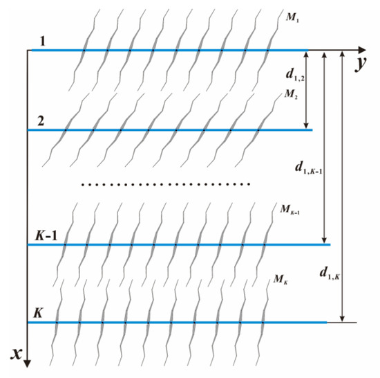
Figure 1.
Schematic diagram of horizontal well group layout.
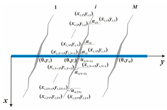
Figure 2.
A schematic diagram of the main fracture dispersion of fractured horizontal wells.
- (2)
- The determination of micro-segment coordinates for primary fractures
For the k-th horizontal well, the primary fractures are sequentially numbered from 1 to Mk (left to right). Each primary fracture is discretized into micro-segments (units) along its left wing (negative-y side) and right wing (positive-y side), with a total of 2N micro-segments per fracture: Left-wing micro-segments: Numbered 1 to N (extending outward from the wellbore). Right-wing micro-segments: Numbered N + 1 to 2N (extending outward from the wellbore). The total number of primary fracture micro-segments for the k-th well is 2 × N × Mk.
The micro-segment coordinates for primary fractures (1 ≤ j ≤ N):
where
The micro-segment coordinates for primary fractures (N + 1 ≤ j ≤ 2N):
where
- 2.
- Pressure Response Derivation
Based on the conductivity contrast between different flow channels within the primary fractures, the flow regimes can be categorized into four types: shale channel conductivity > both coal and tight sandstone channel conductivity; shale channel conductivity ≤ both coal and tight sandstone channel conductivity; coal channel conductivity < shale channel conductivity ≤ tight sandstone channel conductivity; and tight sandstone channel conductivity < shale channel conductivity ≤ coal channel conductivity. Accordingly, the pressure response derivation for transitional marine–terrestrial fractured horizontal well groups must consider these four distinct flow regimes. This study selects the third scenario (where coal channel conductivity < shale channel conductivity ≤ tight sandstone channel conductivity) as the representative case for the model development.
The pressure drop induced at the tip of the m-th primary fracture on the k-th well by all primary fractures from K wells in the shale channel is expressed as
The pressure drop induced at the tip of the m-th primary fracture on the k-th well by all primary fractures from K wells in the coal channel is expressed as
The pressure drop induced at the tip of the m-th primary fracture on the k-th well by all primary fractures from K wells in the tight sandstone channel is expressed as
The transformed flow equation for the shale channel in primary hydraulic fractures after the Laplace transformation is expressed as
The transformed flow equation for the coal channel in primary hydraulic fractures after the Laplace transformation is expressed as
The transformed flow equation for the tight sandstone channel in primary hydraulic fractures after the Laplace transformation is expressed as
By combining Equations (6) and (10)–(12), the pressure expression at the wellbore of the m-th hydraulic fracture on the k-th well can be derived as
- 3.
- Wellbore Pressure Solution and Gas Production in Multi-Fractured Horizontal Wells
Assuming a uniform flowing pressure at the wellbore for all fractures on the k-th well (where k = 1, 2, …, K)
The flow rate normalization criterion for the k-th well is specified as follows:
Combining Equations (14) and (15) yields a system of linear equations for solving the horizontal wellbore pressure:
In the equation
It should be specifically noted that Fm’,i’ and fmi vary depending on the flow regimes of the three main fracture channels, as detailed below:
By solving Equation (16), the dimensionless bottomhole flowing pressure for the k-th well (k = 1, 2, …, K) can be obtained. Then, by applying Duhamel’s principle [28], the expression for the dimensionless bottomhole flowing pressure of the k-th well, incorporating wellbore storage effects and skin effects, can be derived as follows:
where Sc—skin factor and CD—dimensionless wellbore storage coefficient.
Performing an inverse perturbation transformation on Equation (17) yields . Subsequently, through the relational expression between and [29]
Parameter can be obtained. Finally, (the dimensionless production rate of the k-th well) is determined through the Stehfest numerical inversion [30] of .
It should be noted that the model developed in this study can readily account for the heterogeneity among different controlled regions of horizontal wells. The petrophysical parameters for each horizontal well’s drainage area can be assigned based on actual formation property variations. The model is not applicable to massive shale formations.
3. Model Validation
In the Ordos Basin, there are only a few horizontal wells in the marine–continental transitional facies that have been exploited, and they are spaced far apart. As a result, there is a lack of production data for well groups in this facies. In addition, most of the productivity models for fractured horizontal wells proposed by scholars at home and abroad are for single reservoirs and single wells and are not comparable. Therefore, this model is transformed into a model for the well groups of fractured horizontal wells in shale gas; that is, the production data of well groups of fractured horizontal wells in shale gas is used to verify this model.
The model’s predictive capability was rigorously tested using a tri-well pad in Sichuan’s Longmaxi Formation (Table 1). By employing an adaptive ensemble smoother algorithm, the inter-well distances were systematically modified to minimize the normalized root-mean-square error (NRMSE) between simulated post-fracturing production profiles and field observations, ultimately converging to a 7.2% average discrepancy threshold. The fitted parameters included important parameters, such as the main fracture conductivity of the horizontal well and the actual fracture length of each main fracture of each well. The completion and treatment parameters for the three study wells, along with the optimized modeling parameters obtained through production matching, are summarized in Table 2. The well spacing between the three wells is all 300 m, and the specific distribution is shown in Figure 3.

Table 1.
Basic parameters of reservoirs.
Table 2.
Fracturing parameters of production wells.
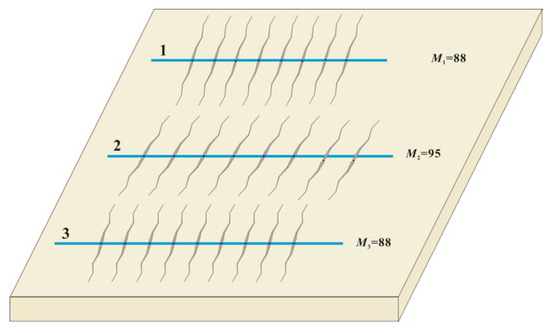
Figure 3.
The relative positions of the three wells.
The production prediction results of the three wells were compared with the actual production data, as shown in Figure 4, Figure 5 and Figure 6. From these three figures, the production decline curves obtained by the model established in this paper generally have a good match with the real-time production decline trends reflected in the production data. For Well 1, the cumulative gas production after 1421 days of production was 6.73 × 10⁷ m3, while the cumulative gas production simulated by the model in this paper was 6.72 × 10⁷ m3, with a difference of 0.1%. For Well 2, the cumulative gas production after 1421 days of production was 7.72 × 10⁷ m3, while the cumulative gas production simulated by the model in this paper was 7.62 × 10⁷ m3, with a difference of 1.3%. For Well 3, the cumulative gas production after 1421 days of production was 8.37 × 10⁷ m3, while the cumulative gas production simulated by the model in this paper was 8.13 × 10⁷ m3, with a difference of 2.95%. The field verification shows that simulated production curves for all three wells fall within 10–15% of actual measurements, validating the model’s predictive capability. The consistent underprediction trend suggests the need to incorporate fracture network complexity, particularly the near-wellbore diversion effects and induced micro-fractures beyond main planar fractures.
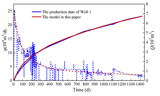
Figure 4.
Production data fitting curve of Well 1.
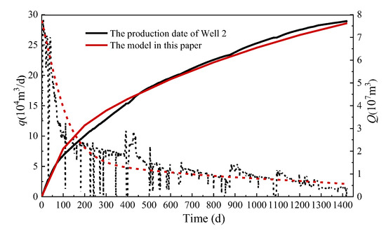
Figure 5.
Production data fitting curve of Well 2.
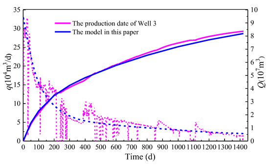
Figure 6.
Production data fitting curve of Well 3.
4. Analysis of Influencing Factors
In the marine–terrestrial transitional shale reservoir, Well 1 was the first long-fractured well with large fracture spacing to be put into production; Well 2 was a short-fractured well with small fracture spacing that was put into production one year after Well 1; and Well 3 was a new well (adjustment well) to be put into production between the two old wells. The relative positions of these three wells are shown in Figure 7, and the related parameters are listed in Table 3 and Table 4. In Figure 7, labels 1–3 correspond to horizontal Wells 1 through 3, while M indicates the number of fractures associated with each respective well. The fracture distribution patterns and conductivity profiles for each of the three wells are presented in Figure 8 and Figure 9, Figure 10, Figure 11 and Figure 12, respectively. In Figure 8, the x-axis represents the length of the horizontal well pattern, while the y-axis indicates the fracture length. For Figure 9, Figure 10, Figure 11 and Figure 12, the x-axis similarly denotes the horizontal well pattern length, with the y-axis representing fracture conductivity. The spacing between the three wells is set as follows: d1,3 = d2,3 = 400 m. The previously validated multi-stage fractured well interference model was applied to determine optimal completion parameters for the adjustment well, utilizing petrophysical and geomechanical inputs from Table 3 through an ensemble-based optimization workflow.
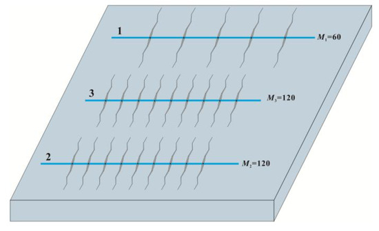
Figure 7.
The location of adjustment wells.
Table 3.
Geological parameters of production wells.
Table 4.
Fracturing parameters of three wells.
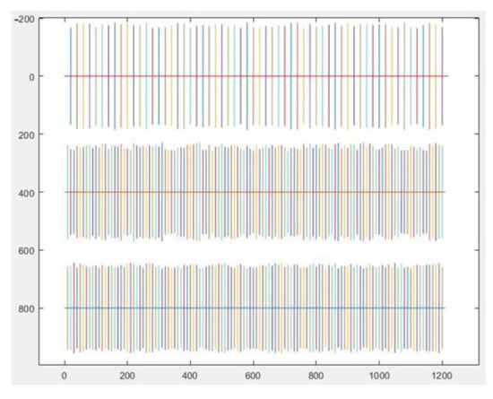
Figure 8.
The hydraulic fracture distribution of the three wells.
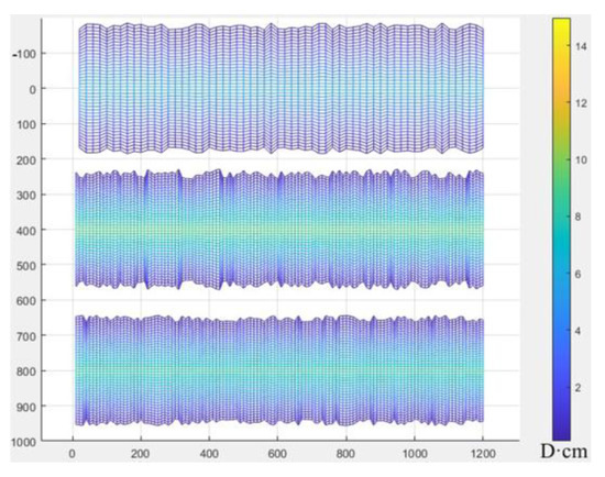
Figure 9.
Distribution of coalbed conductivity for three wells.
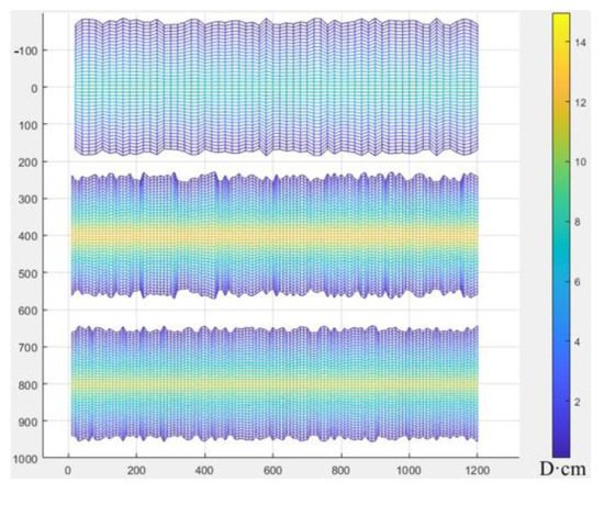
Figure 10.
Distribution of shale conductivity for three wells.
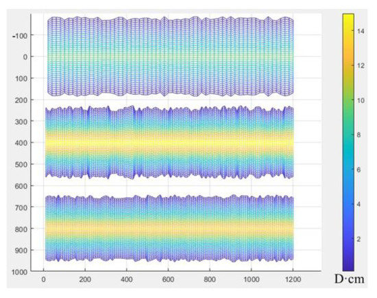
Figure 11.
Distribution of tight sandstone conductivity for three wells.
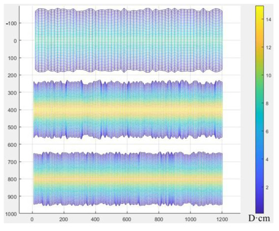
Figure 12.
Distribution of average conductivity for three wells.
4.1. The Optimization of the Spacing for the Infill Well
From the previous literature [31], it is known that the optimal opening time for adjustment wells is between 2.85 and 3 years. Therefore, the opening time is set to 3 years. With Wells 1 and 2 positionally constrained (d1,2 = d1,3 + d2,3 = 800 m), a parametric analysis was conducted by systematically varying inter-well distances d12 and d13. This generated production profiles (daily rate q, cumulative Q vs. time t) across spacing scenarios, with results presented in Figure 13, Figure 14 and Figure 15.
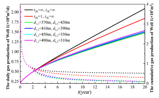
Figure 13.
The regimes of the inter-well spacing of the infill well on the production of Well 1.
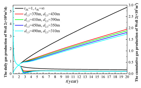
Figure 14.
The regimes of the inter-well spacing of the infill well on the production of Well 2.
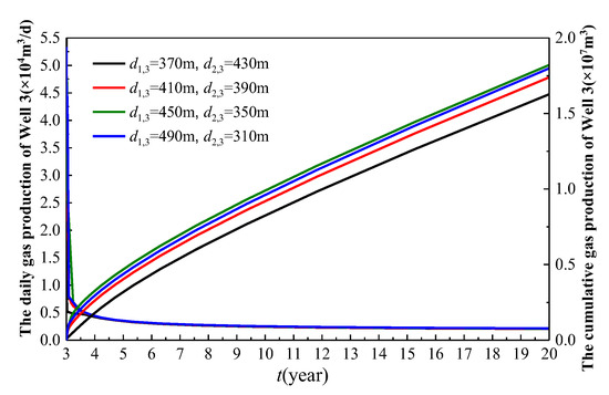
Figure 15.
The regimes of the inter-well spacing of the infill well on the production of Well 3.
In Figure 13, the black curve represents the production of Well 1 when it is the sole producer (Wells 2 and 3 remain shut-in). The red curve depicts the production behavior of Well 1 after Well 2 is brought online following one year of the production from Well 1. The remaining curves demonstrate the production performance of Well 1 under varying well spacing configurations, where Well 2 is brought online 1 year after Well 1’s initial production, and Well 3 commences production 3 years after Well 1’s startup (i.e., 2 years after Well 2’s activation). As illustrated in Figure 13, the gas production of Well 1 increases as the distance d1,3 between Well 1 and Well 3 grows. This phenomenon can be attributed to the reduced interference from Well 3 on Well 1 as the distance increases, thereby enhancing the productivity of Well 1. In the scenario where only Well 2 is operational without Well 3, the cumulative gas production of Well 1 over a 20-year period is 3.28 × 10⁷ m3. When the well spacing d1,3 is set at 370 m, 410 m, 450 m, and 490 m, the corresponding 20-year cumulative gas production of Well 1 is 2.549 × 10⁷ m3, 2.593 × 10⁷ m3, 2.635 × 10⁷ m3, and 2.674 × 10⁷ m3, respectively. Compared to the scenario with only Well 2 in operation, the cumulative gas production of Well 1 decreases by 22.3%, 20.9%, 19.7%, and 18.5% for the respective spacing. The cumulative gas production increases by 1.73%, 1.59%, and 1.48% as the spacing increases from 370 m to 490 m. The average increase rate per meter (cumulative gas production increase/increased spacing) is 0.043%, 0.04%, and 0.037%, respectively. The trend of increasing and then decreasing rates suggests that an optimal value exists for the well spacing d1,3.
As illustrated in Figure 15, the gas production of Well 3 increases as the well spacing d1,3 becomes larger. Specifically, the closer Well 3 is to Well 2 and the farther it is from Well 1, the higher its gas production. This indicates that the influence of Well 1 on Well 3 is more significant than that of Well 2. Although Well 1 is a long-fractured well with large spacing, it was put into production earlier than Well 2. By the time Well 3 began production, Well 1 had already been producing for 3 years, while Well 2 had only been operational for 2 years. Consequently, the cumulative gas production of Well 1 over 3 years exceeded that of Well 2 over 2 years. Therefore, when Well 3 commenced production, the formation pressure near Well 1 was lower compared to that near Well 2. As a result, the closer Well 3 is to Well 1, the lower the formation pressure, leading to the reduced gas production from Well 3. From the perspective of cumulative gas production, when the well spacing d1,3 is set at 370 m, 410 m, 450 m, and 490 m, the cumulative gas production of Well 3 over 17 years is 1.627 × 10⁷ m3, 1.74 × 10⁷ m3, 1.821 × 10⁷ m3, and 1.799 × 10⁷ m3, respectively. The increase in the cumulative gas production is 6.92%, 4.67%, and −1.2%. The trend of the increasing and then decreasing cumulative gas production suggests that there is an optimal value for the well spacing d1,3.
The analysis of the aggregate production from the three-well system reveals an inverse relationship between the spacing (d13) and individual well performance: Wells 1 and 3 exhibit positive EUR correlations (+0.8%/10 m spacing increase), whereas Well 2 shows a compensatory decline (−1.2%/10 m), as quantified in Figure 14. Therefore, using the total cumulative gas production of the three wells as the objective function, an optimal value for the well spacing must exist. Table 5 compiles the spacing-dependent EUR data for the three-well system. Figure 16 plots the aggregated production curve versus the d13 spacing, peaking at 450 m—establishing the optimal configuration as d13 = 450 m with d23 = 350 m for maximum recovery.
Table 5.
Cumulative gas production of three wells (different well spacings).
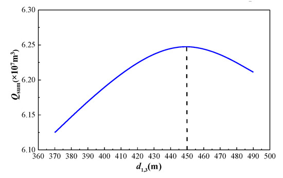
Figure 16.
Optimization results of the spacing of the infill well.
4.2. The Optimization of the Main Fracture Conductivity for the Infill Well
From the preceding analysis, we have determined the spacing for the infill well. Next, we will investigate the impact of the main fracture conductivity (Cfd_3) of the infill well on the performance of the well group. By varying the main fracture conductivity Cfd_3, we can obtain the curve characteristics of the daily production (q), cumulative production (Q), and time (t) for the three wells under different levels of main fracture conductivity. The resulting curves are illustrated in Figure 17, Figure 18 and Figure 19.
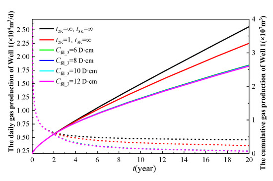
Figure 17.
The influence of the main fracture conductivity of the infill well on the production of Well 1.
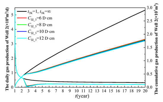
Figure 18.
The influence of the main fracture conductivity of the infill well on the production of Well 2.
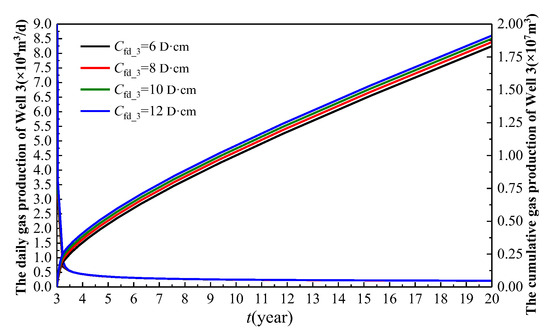
Figure 19.
The influence of the main fracture conductivity of the infill well on the production of Well 3.
In Figure 17, the black curve represents the production of Well 1 when it is the sole producer (Wells 2 and 3 remain shut-in). The red curve depicts the production behavior of Well 1 after Well 2 is brought online following one year of production of Well 1. The remaining curves demonstrate the production performance of Well 1 under varying well spacing configurations, where Well 2 is brought online 1 year after Well 1’s initial production, and Well 3 commences production 3 years after Well 1’s startup (i.e., 2 years after Well 2’s activation). As illustrated in Figure 17 and Figure 18, the greater the main fracture conductivity (Cfd_3) of the infill well, the lower the production of Well 1 and Well 2. This is because a higher main fracture conductivity creates an easier flow of natural gas from the formation into the horizontal wellbore of the infill well, indirectly reducing the natural gas production of the two older wells. Specifically, when Cfd_3 is set to 6D·cm, 8D·cm, 10D·cm, and 12D·cm, the cumulative gas production of Well 1 over 20 years is 2.635 × 10⁷ m3, 2.625 × 10⁷ m3, 2.614 × 10⁷ m3, and 2.604 × 10⁷ m3, respectively, resulting in a total decline of 1.2%. Similarly, the cumulative gas production of Well 2 over 19 years is 1.809 × 10⁷ m3, 1.789 × 10⁷ m3, 1.77 × 10⁷ m3, and 1.751 × 10⁷ m3, respectively, leading to a total decline of 3.3%.
As illustrated in Figure 19, the greater the main fracture conductivity (Cfd_3) of the infill well, the higher the gas production of Well 3. This is because a higher main fracture conductivity results in a more efficient flow channel for natural gas from the formation to the horizontal wellbore, thereby increasing the gas well production. From the cumulative gas production data, when Cfd_3 is set to 6D·cm, 8D·cm, 10D·cm, and 12D·cm, the cumulative gas production of Well 3 over 17 years is 1.832 × 10⁷ m3, 1.863 × 10⁷ m3, 1.889 × 10⁷ m3, and 1.913 × 10⁷ m3, respectively. The cumulative gas production increases by 1.7%, 1.4%, and 1.3%, with a total increase of 4.42%. The gradually decreasing rate of the increase in the cumulative gas production suggests that there is an optimal value for the main fracture conductivity Cfd_3 of the adjustment well.
Considering the cumulative gas production of the three wells, it is observed that as the main fracture conductivity (Cfd_3) of the infill well increases, the production of the two older wells decreases, while the production of the infill well increases. Consequently, the total cumulative gas production of the well group initially rises and then declines, indicating the existence of an optimal value for the main fracture conductivity of the adjustment well. By using the cumulative gas production of the three wells as the objective function, the optimal main fracture conductivity Cfd_3 can be determined. The cumulative gas production of the three wells under different values of Cfd_3 is summarized in Table 6. The curve representing the total cumulative gas production of the three wells as a function of the main fracture conductivity Cfd_3 is depicted in Figure 20. As shown in Figure 20, the curve reaches its peak when the main fracture conductivity Cfd_3 is 7.8D·cm. Therefore, the optimal main fracture conductivity for the adjustment well is 7.8D·cm.
Table 6.
Cumulative gas production of three wells corresponding to different main fracture conductivities.
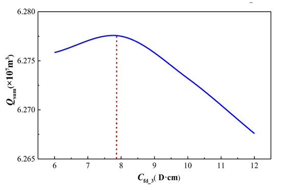
Figure 20.
Optimization results of the main fracture conductivity of the infill well.
4.3. The Optimization of the Number and Spacing of Main Fractures for the Infill Well
From the preceding analysis, we have determined the optimal main fracture conductivity of the infill well. Next, we will investigate the influence of the number of main fractures (mcu_3) and the corresponding spacing on the performance of the well group. By varying the number of main fractures mcu_3, we can obtain the curve characteristics of the daily production (q), cumulative production (Q), and time (t) for the three wells under different numbers of main fractures. The resulting curves are illustrated in Figure 21, Figure 22 and Figure 23.
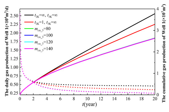
Figure 21.
The influence of the number of main fractures for the infill well on the production of Well 1.
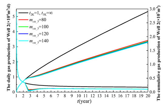
Figure 22.
The influence of the number of main fractures for the infill well on the production of Well 2.
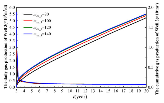
Figure 23.
The influence of the number of main fractures for the infill well on the production of Well 3.
In Figure 21, the black curve represents the production of Well 1 when it is the sole producer (Wells 2 and 3 remain shut-in). The red curve depicts the production behavior of Well 1 after Well 2 is brought online following one year of production from Well 1. The remaining curves demonstrate the production performance of Well 1 under varying well spacing configurations, where Well 2 is brought online 1 year after Well 1’s initial production, and Well 3 commences production 3 years after Well 1’s startup (i.e., 2 years after Well 2’s activation). As illustrated in Figure 21, as the number of main fractures (mcu_3) in the infill well increases, the production of Well 1 gradually decreases. The greater the number of main fractures, the more significant the inter-well interference between Well 3 and Well 1, leading to a lower production rate for Well 1. However, overall, the impact of the main fracture cluster number on Well 1 is relatively minor. This is because Well 1 is already in the middle to late stages of production and is located at a considerable distance from Well 3, thereby limiting the extent of the interference. When only Well 2 is present without Well 3, the cumulative gas production of Well 1 over 20 years is 3.28 × 10⁷ m3. With mcu_3 set to 80, 100, 120, and 140, the cumulative gas production of Well 1 over 20 years is 2.643 × 10⁷ m3, 2.638 × 10⁷ m3, 2.635 × 10⁷ m3, and 2.633 × 10⁷ m3, respectively. Compared to the scenario where only Well 2 is producing, the cumulative gas production of Well 1 decreases by 19.4%, 19.6%, 19.7%, and 19.73%, respectively. As mcu_3 increases from 80 to 140, the reduction in the cumulative gas production of Well 1 is 0.212%, 0.115%, and 0.077%, respectively. The decreasing trend in the reduction rate suggests that there is an optimal value for the number of main fracture clusters (mcu_3) in the adjustment well.
As illustrated in Figure 22, as the number of main fractures (mcu_3) of the infill well increases, the production of Well 2 gradually decreases. This is because a higher number of main fractures leads to greater inter-well interference between Well 3 and Well 2, thereby reducing the production of Well 2. Without Well 3, the cumulative gas production of Well 2 over 19 years is 2.91 × 10⁷ m3. When mcu_3 is set to 80, 100, 120, and 140, the cumulative gas production of Well 2 over 19 years is 1.867 × 10⁷ m3, 1.832 × 10⁷ m3, 1.809 × 10⁷ m3, and 1.794 × 10⁷ m3, respectively. Compared to the scenario without Well 3, the cumulative gas production of Well 2 decreases by 35.8%, 37%, 37.8%, and 38.4%, respectively. As mcu_3 increases from 80 to 140, the reduction in the cumulative gas production of Well 2 is 1.875%, 1.255%, and 0.829%, respectively. The decreasing trend in the reduction rate suggests that there is an optimal value for the number of main fracture clusters (mcu_3) of the infill well.
As shown in Figure 23, as the number of main fractures (mcu_3) of the infill well increases, the gas production of Well 3 also increases relatively. This is because as the main fractures’ number increases, the cluster spacing decreases, leading to an increase in the control area of the horizontal well on the formation and more natural gas entering the wellbore through the main fractures. In terms of cumulative gas production, when mcu_3 is set to 80, 100, 120, and 140, the cumulative gas production of Well 3 over 17 years is 1.743 × 10⁷ m3, 1.8 × 10⁷ m3, 1.832 × 10⁷ m3, and 1.843 × 10⁷ m3, respectively. The increase in the cumulative gas production is 3.27%, 1.78%, and 0.6%, with a total increase of 5.74%. The gradual decrease in the rate of the increase in the cumulative gas production of Well 3 indicates that there is an optimal value for the number of main fractures (mcu_3) and the corresponding fracture spacing of the infill well.
The production analysis reveals an inverse relationship between the infill well fracture density (mcu_3) and the parent well performance. While Well 3’s EUR increases by 1.2%/fracture, Wells 1–2 exhibit a 0.8%/fracture decline, creating a bell-shaped total production curve peaking at mcu_3 = 12 (Table 7, Figure 24). These optimally balance the stimulation efficiency versus interference. As shown in Figure 24, the peak of the curve occurs when mcu_3 is equal to 120. Therefore, the optimal number of main fracture clusters for the infill well is 120, with a corresponding spacing of 10 m (given that the horizontal section length of infill Well 3 is 1200 m).
Table 7.
Cumulative gas production of three wells corresponding to different numbers of main fractures.
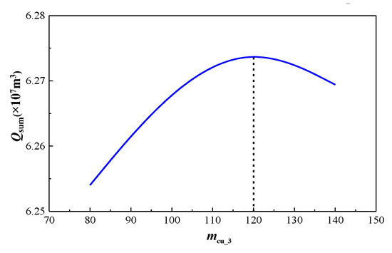
Figure 24.
Optimization results of the number of main fractures for the infill well.
5. Conclusions
By taking into account the influence of the complex fracture morphology, the productivity model of fractured horizontal well groups in shale gas reservoirs for predicting the production decline law has been established. The main conclusions are summarized as follows:
- (1)
- Based on the seepage model of the horizontal single well in the marine–continental transitional phase fracturing, the productivity model of the horizontal well group in the marine–continental transitional phase fracturing considering the stress sensitivity effect of the natural fractures, the complex fracture morphology and inter-well interference is established. It can be used to predict the productivity of multiple interfering horizontal wells in the marine–continental transitional phase shale reservoirs and then can be used to optimize the relevant parameters of the infill wells in the marine–continental transitional phase shale gas reservoirs. In the horizontal well group, the pressure interference between wells is mainly the inter-fracture interference of the main fractures of the horizontal wells on each other; that is, the inter-well interference is transmitted through the main fractures of each well.
- (2)
- The field validation using Sichuan shale gas production data demonstrates the model’s accuracy in predicting the post-fracturing performance for three co-developed horizontal wells. Simulation results align with the actual production with a small error margin, confirming the model reliability for this reservoir type.
- (3)
- The established model was utilized to optimize three parameters of the infill wells in the marine–terrestrial transitional phase. The optimization results indicated that the closer the infill well was to the old well, the lower the production of the corresponding old well would be; the farther the infill well was from the first large-spacing long-fractured well put into production, the higher the production of the infill well would be. There was an optimal relative distance between the infill well and the two old wells: d1,3 = 450 m and d2,3 = 350 m. When the horizontal wellbore length was fixed, the greater the main fractures of the infill well and the smaller the corresponding fracture spacing, the higher the production of the infill well would be, and the lower the production of the two old wells would be. For the infill well with a horizontal section length of 1200 m, the optimal number of main fractures was 120, and the corresponding optimal fracture spacing was 10 m. The greater the conductivity of the main fractures of the infill well, the lower the production of the two old wells would be, and the higher the production of the infill well would be. There was an optimal value of 7.8D·cm for the conductivity of the main fractures of the infill well.
Author Contributions
Writing—original draft preparation, G.L.; writing—review and editing, D.L. and J.Z.; Conceptualization, L.R. and R.L.; validation, B.G. and W.Z.; formal analysis, M.C.; resources, J.W. All authors have read and agreed to the published version of the manuscript.
Funding
The project is supported by the Chuanqing drilling Engineering Co., Ltd. project (Number CQ2023B-30-4-4), Science and Technology Cooperation Project of the CNPC-SWPU Innovation alliance (2020CX030201), National Natural Science Foundation of China “Investigation of efficient hydraulic fractures-network construction theory and method for deep/ultra-deep horizontal shale gas well”(U21B2071), and National Natural Science Foundation of China “Fundamental Research on Nano-Supercritical CO2 Fracturing-Replacement-Displacement Synergistic Enhanced Shale Gas Recovery” (U24A2084).
Data Availability Statement
All data generated or analyzed during this study are included in this published article.
Conflicts of Interest
The authors declare that this study received funding from the Chuanqing drilling Engineering Co., Ltd. project (Number CQ2023B-30-4-4), Science and Technology Cooperation Project of the CNPC-SWPU Innovation alliance (2020CX030201). Authors Gaomin Li, Dengyun Lu, Bin Guan, Wengao Zhou, and Minzhong Chen were employed by the CNPC Chuanqing Drilling Engineering Company Limited. Author Jianjun Wu was employed by the CNPC Coalbed Methane Company Limited that could be construed as a potential conflict of interest.
Nomenclature
The Declaration of Symbols and Variables
| Cfgi | The composite compressibility of natural fracture systems under initial conditions, Pa−1 |
| CD | The dimensionless wellbore storage factor, dimensionless |
| D | The molecular diffusivity, m2/s |
| f(s) | The main function of the variable s |
| h1 | The thickness of the shale reservoir, m |
| h2 | The thickness of the coalbed reservoir, m |
| h3 | The thickness of the tight sandstone reservoir, m |
| ku,i | The shunt coefficients of ith main fracture of uth Well |
| kuij0 | The original shunt coefficients of jth section of ith main fracture of uth Well |
| kuij | The shunt coefficients of jth section of ith main fracture of uth Well |
| L | Reference length, m |
| PL | Langmuir pressure, Pa |
| pw | Flowing bottomhole pressure, Pa |
| qsc | The reference total flow rate for fractured horizontal Wells, m3/s |
| Dimensionless reference total flow in Laplace space for kth Well | |
| The dimensionless flow over the reference length of the discrete segment for the uth Well | |
| qfm | The gas flow of the mth main fracture, m3/s |
| R | The radius of the matrix element, m |
| r’ecn | The equivalent seepage radius of the (n−1)th section of the cth secondary fracture connected to the mth hydraulic fracture, m |
| recn | The equivalent seepage radius at the bottom of the nth section of the cth secondary fracture connected to the mth main fracture, m |
| rec0 | The equivalent seepage radius at the junction of the cth secondary fracture and the mth main fracture, m; |
| rD | Dimensionless radius |
| Sc | The skin factor, dimensionless |
| s | Complex parameters in Laplace transform |
| tD | Dimensionless time |
| Vi | The gas adsorption capacity of the matrix system under initial conditions, m3/kg |
| VD | Dimensionless adsorption capacity of matrix system |
| Dimensionless adsorption of matrix system in Laplace space | |
| VE | The amount of gas adsorption at adsorption equilibrium, m3/kg |
| VL | Langmuir volume, m3/kg; |
| xwDu,i | The dimensionless abscissa of any element on the ith main fracture for the uth Well |
| xu,fli | The half-length of ith main fracture of the uth Well |
| xu,fri | The half-length of ith main fracture of the uth Well |
| yu,wDi | The dimensionless ordinate of any element on the ith main fracture of the uth Well(1 ≤ j ≤ N: g = N − j + 1, N + 1 ≤ j ≤ 2N: g = j) |
| rek | The outer diameter length of the equivalent radius of the plane radial flow at the kth (k = 1, 2, …, n) section of the mth main fracture, m |
| rek,(k−1) | The inside diameter length of the equivalent radius of the plane radial flow at the kth (k = 1, 2, …, n) section of the mth main fracture, m; |
| μ | The gas viscosity in fracture systems at average temperature and pressure, Pa·s |
| φf(p) | The pseudo-pressure of natural fracture systems, Pa2/(Pa·s) |
| φfD | Dimensionless pseudo-pressure of natural fracture system |
| φm(p) | The pseudo-pressure of the matrix system, Pa2/(Pa·s) |
| φi | The pseudo-pressure of natural fracture systems under initial conditions, Pa2/(Pa·s) |
| βg | A parameter that positively correlates with the stress sensitivity coefficient, |
| ω | The storativity ratio, dimensionless |
| λ | The inter-porosity coefficient, dimensionless |
| γD | The dimensionless stress sensitive factor, dimensionless |
| τ | Pore tortuosity, m |
| The dimensionless pseudo-pressure of natural fracture system after Laplace transform and perturbation transform | |
| σ | The desorption index, dimensionless |
| Cfgi | The composite compressibility of natural fracture systems under initial conditions, Pa−1 |
| CD | The dimensionless wellbore storage factor, dimensionless |
| Subscript | Superscript | ||||||
| D | Dimensionless | - | Laplace space | ||||
| i | Initial condition | ′ | Parameters in coalbed model | ||||
| sc | Under standard conditions | ″ | Parameters in tight sandstone model | ||||
| f | Natural fracture (cleat) system | ||||||
| m | Matrix system | ||||||
| g | Gas | ||||||
| w | Well | ||||||
| ts | Tight sandstone layer |
References
- Qiu, Z.; Zou, C.N.; Benjamin, J.W.M.; Xiong, Y.J.; Tao, H.F.; Lu, B.; Liu, H.L.; Xiao, W.J.; Simon, W.P. A nutrient control on expanded anoxia and global cooling during the Late Ordovician mass extinction. Commun. Earth Environ. 2022, 3, 82. [Google Scholar] [CrossRef]
- Qiu, Z.; Zou, C.N. Unconventional Petroleum Sedimentology: Connotation and prospect. Acta Sedimentol. Sin. 2020, 38, 1–29. [Google Scholar] [CrossRef]
- Xu, J.C.; Guo, C.H.; Wei, M.Z.; Jiang, R.Z. Production performance analysis for composite shale gas reservoir considering multiple transport mechanisms. J. Nat. Gas Sci. Eng. 2015, 26, 382–395. [Google Scholar] [CrossRef]
- Guo, W.; Gao, J.L.; Li, H.; Kang, L.X.; Zhang, J.W.; Liu, G.H.; Liu, Y.Y. The geological and production characteristics of marine-continental transitional shale gas in China: Taking the example of shale gas from Shanxi Formation in Ordos Basin and Longtan Formation in Sichuan Basin. Miner. Explor. 2023, 14, 448–458. [Google Scholar] [CrossRef]
- Ma, Y.S.; Cai, X.Y.; Zhao, P.R. China’s shale gas exploration and development: Understanding and practice. Pet. Explor. Dev. 2018, 45, 561–574. [Google Scholar] [CrossRef]
- Ma, X.H.; Zhang, X.W.; Xiong, W.; Liu, Y.Y.; Gao, J.J.; Yu, R.Z.; Sun, Y.P.; Wu, J.; Kang, L.X.; Zhao, S.P. Prospects and challenges of shale gas development in China. Pet. Sci. Bull. 2023, 8, 491–501. [Google Scholar] [CrossRef]
- Zou, C.N.; Dong, D.Z.; Wang, Y.M.; Li, X.J.; Huang, J.L.; Wang, S.F.; Guan, Q.Z.; Zhang, C.C.; Wang, H.Y.; Liu, H.L.; et al. Shale gas in China: Characteristics, challenges and prospects (II). Pet. Explor. Dev. 2016, 43, 166–178. [Google Scholar] [CrossRef]
- Xu, Y.; Lei, Q.; Chen, M.; Wu, Q.; Yang, N.Y.; Weng, D.W.; Li, D.Q.; Jiang, H. Progress and development of volume stimulation techniques. Pet. Explor. Dev. 2018, 45, 874–887. [Google Scholar] [CrossRef]
- Wei, Y.S.; Wang, J.L.; Qi, Y.D.; Jin, Y.Q. Optimization of shale gas well pattern and spacing. Nat. Gas Ind. 2018, 38, 129–137. [Google Scholar]
- Zhao, Q.; Wang, H.Y.; Sun, Q.P.; Jiang, X.C.; Yu, R.Z.; Kang, L.X.; Wang, X.F. A logical growth model considering the influence of shale gas reservoirs and development characteristics. Nat. Gas Ind. 2020, 40, 77–84. [Google Scholar] [CrossRef]
- Gupta, J.; Zielonka, M.; Albert, R.A.; Wadood, E.R.; Heather, A.B.; Nancy, H.C. Integrated methodology for optimizing development of unconventional gas resources. In Proceedings of the SPE Hydraulic Fracturing Technology Conference, The Woodlands, TX, USA, 6–8 February 2012. [Google Scholar]
- Roussel, N.P.; Florez, H.; Rodriguez, A.A. Hydraulic fracture propagation from infill horizontal wells. In Proceedings of the SPE Annual Technical Conference and Exhibition, New Orleans, LA, USA, 30 September–2 October 2013. [Google Scholar]
- Marongiu-Porcu, M.; Lee, D.; Shan, D.; Morales, A. Advanced modeling of interwell fracturing interference: An Eagle Ford Shale oil study. In Proceedings of the SPE Annual Technical Conference and Exhibition, Houston, TX, USA, 28–30 September 2015. [Google Scholar]
- Huang, J.; Ma, X.; Safari, R.; Mutlu, U.; McClure, M. Hydraulic fracture design optimization for infill wells: An integrated geomechanics workflow. In Proceedings of the 49th U.S. Rock Mechanics/Geomechanics Symposium, San Francisco, CA, USA, 28 June–1 July 2015. [Google Scholar]
- Jacobs, T. Oil and Gas Producers Find Frac Hits in Shale Wells a Major Challenge. J. Pet. Technol. 2017, 69, 29–34. [Google Scholar] [CrossRef]
- Zheng, W.; Xu, L.; Moncada, K.; Xu, T.; Pankaj, P.; Sinha, H. Production induced stress change impact on infill well flow back operations in Permian Basin. In Proceedings of the SPE Liquids-Rich Basins Conference-North America, Midland, TX, USA, 5–6 September 2018. [Google Scholar]
- Guo, X.; Wu, K.; Killough, J. Investigation of production-induced stress changes for infill well stimulation in Eagle Ford Shale. In Proceedings of the SPE/f1APG/SEG Unconventional Resources Technology Conference (URTeC), Austin, TX, USA, 24–26 July 2017. [Google Scholar]
- Safari, R.; Lewis, R.; Ma, X.; Uno, M.; Ahmad, G. Infill-well fracturing optimization in tightly spaced horizontal wells. SPE J. 2017, 22, 582–595. [Google Scholar] [CrossRef]
- Zhu, H.Y.; Song, Y.J.; Xu, Y.; Li, K.D.; Tang, X.H. Four-dimensional in-situ stress evolution of shale gas reservoirs and its impact on infill well complex fractures propagation. Acta Pet. Sin. 2021, 42, 1224–1236. [Google Scholar] [CrossRef]
- Li, J.; Liu, L.; Zhu, Y.; Zhao, L.; Chai, X.; Tian, L. A new dynamic model of supply boundary at low pressure in tight gas reservoir. Sci. Rep. 2025, 15, 12178. [Google Scholar] [CrossRef]
- Asghari, M.; Maleki, Z.; Solgi, A.; Ganjavian, M.A.; Kianoush, P. Geohazard impact and gas reservoir pressure dynamics in the Zagros Fold-Thrust Belt: An environmental perspective. Geosyst. Geoenviron. 2025, 4, 100362. [Google Scholar] [CrossRef]
- Wu, H.; Gao, K.; Jian, F.; Nicholas, M.; Walton, W. A novel way to achieve early commercialisation of tight-sand and shale gas fields: Small-scale modularised liquefied natural gas. Aust. Energy Prod. J. 2025, 65, 1–4. [Google Scholar] [CrossRef]
- Wu, Y.; Mi, L.; Zheng, R.; Ma, L.; Feng, X. A practical semi-analytical model for production prediction of fractured tight gas wells with multiple nonlinear flow mechanisms. Arab. J. Sci. Eng. 2025, 50, 4687–4702. [Google Scholar] [CrossRef]
- Tang, Z.; Chen, Z.; Han, J.; Zhao, X.; Chen, Z.; Tan, P. A New tEDFM-Based Analysis of Interference Characterization in Tight Gas Reservoir. Energy 2025, 330, 136669. [Google Scholar] [CrossRef]
- Lin, R.; Li, G.M.; Zhao, J.Z.; Ren, L.; Wu, J.F. Productivity model of shale gas fractured horizontal well considering complex fracture morphology. J. Pet. Sci. Eng. 2025, 208, 109511. [Google Scholar] [CrossRef]
- Jiang, R.Z.; Liu, X.W.; Wang, X.; Gao, Y.H.; Gao, Y.; Huang, Y.S. Unsteady productivity model for multi-branched horizontal wells in coalbed methane reservoir. Pet. Geol. Recovery Effic. 2020, 27, 48–56. [Google Scholar] [CrossRef]
- Dai, X.L. Study on Productivity Evaluation of Fractured Horizontal Well of Tight Gas Reservoir. Master’s Thesis, Southwest Petroleum University, Chengdu, China, 2016. [Google Scholar]
- Jasper, K.; Hartkopf-Froder, C.; Flajs, G.; Littke, R. Evolution of Pennsylvanian (Late Carboniferous) peat swamps of the Ruhr Basin, Germany: Comparison of palynological, coal petrographical and organic geochemical data. Int. J. Coal Geol. 2010, 83, 346–365. [Google Scholar] [CrossRef]
- Mclaughlin, M.R.; Brooks, J.P.; Adeli, A. Characterization of selected nutrients and bacteria from anaerobic swine manure lagoons on sow, nursery, and finisher farms in the Mid-South USA. J. Environ. Qual. 2009, 38, 2422–2430. [Google Scholar] [CrossRef] [PubMed]
- Ross, D.J.; Bustin, R.M. The importance of shale composition and pore structure upon gas storage potential of shale gas reservoirs. Mar. Pet. Geol. 2009, 26, 916–927. [Google Scholar] [CrossRef]
- Ren, L.; Li, G.M.; Zhao, J.Z.; Wu, J.F. Infill well deployment optimization based on a novel multi-well productivity model considering inter-well interference for shale gas reservoir. Pet. Sci. Technol. 2025, 43, 174–201. [Google Scholar] [CrossRef]
Disclaimer/Publisher’s Note: The statements, opinions and data contained in all publications are solely those of the individual author(s) and contributor(s) and not of MDPI and/or the editor(s). MDPI and/or the editor(s) disclaim responsibility for any injury to people or property resulting from any ideas, methods, instructions or products referred to in the content. |
© 2025 by the authors. Licensee MDPI, Basel, Switzerland. This article is an open access article distributed under the terms and conditions of the Creative Commons Attribution (CC BY) license (https://creativecommons.org/licenses/by/4.0/).