
MS-Unet: A Multi-Scale Feature Fusion U-Net for 3D Seismic Fault Detection


Abstract
1. Introduction
2. Materials and Methods
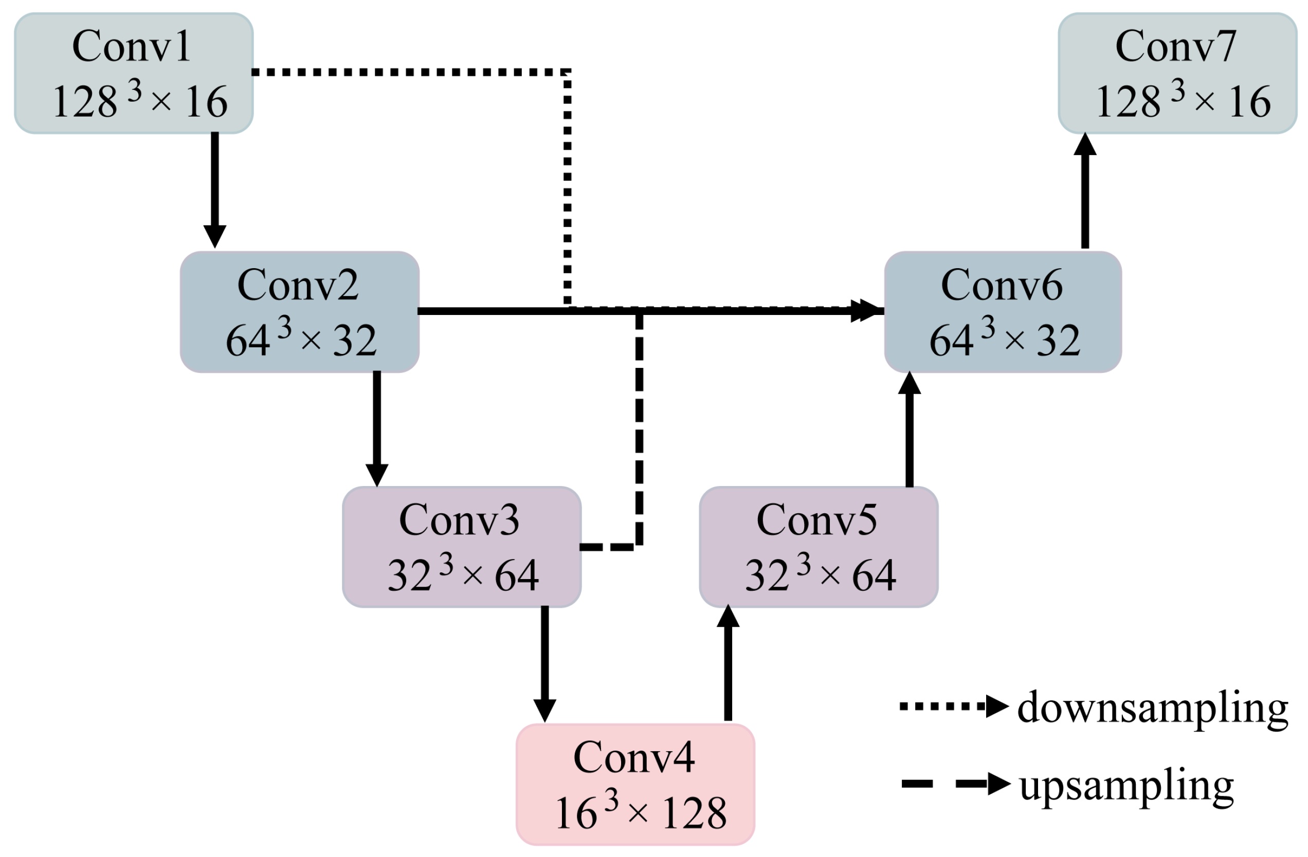
2.1. Overall Architecture
2.2. Network Architecture Details
2.3. Evaluation Indicators
3. Results
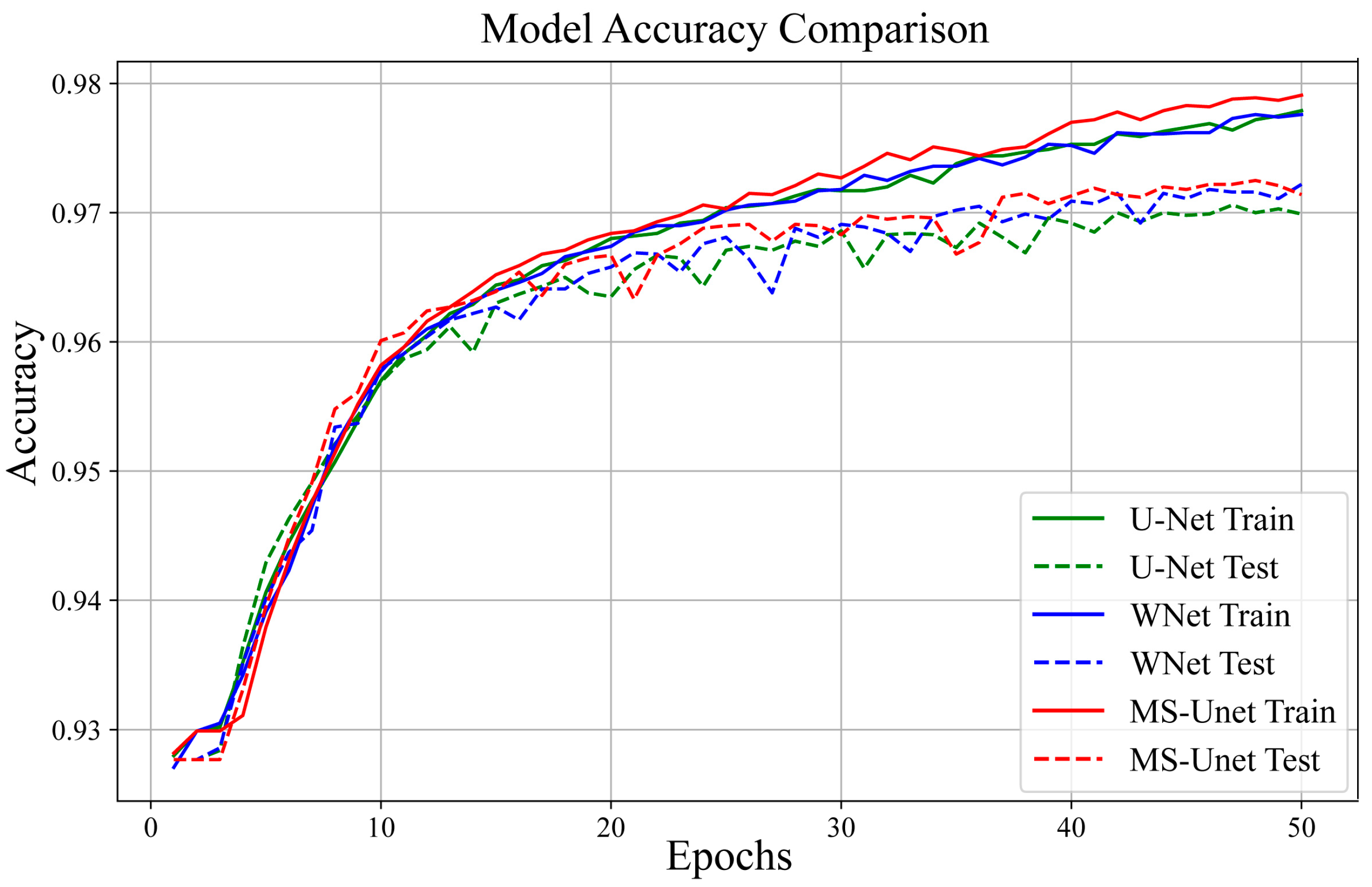
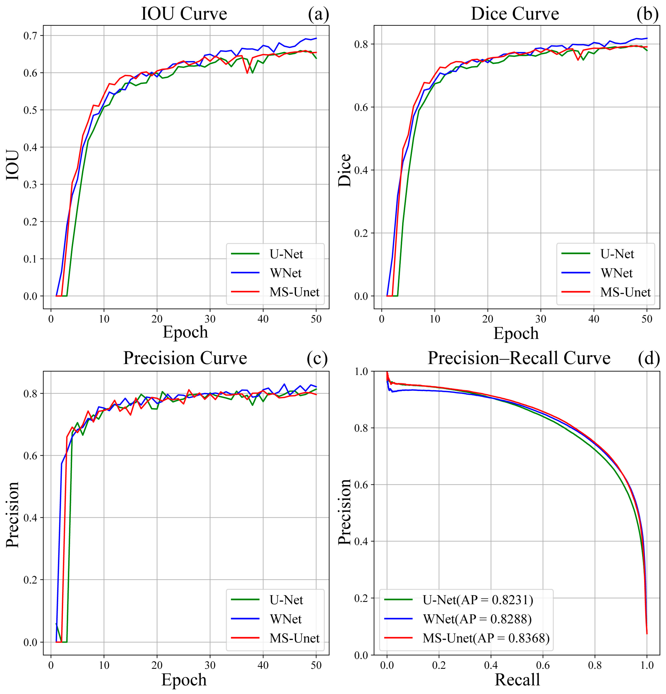
3.1. Synthetic Data
3.2. Three-Dimensional Field Data Examples
4. Conclusions
Author Contributions
Funding
Data Availability Statement
Conflicts of Interest
References
- Fossen, H. Structural Geology; Cambridge University Press: Cambridge, UK, 2016. [Google Scholar]
- An, Y.; Guo, J.; Ye, Q.; Childs, C.; Walsh, J.; Dong, R. Deep Convolutional Neural Network for Automatic Fault Recognition from 3D Seismic Datasets. Comput. Geosci. 2021, 153, 104776. [Google Scholar] [CrossRef]
- Marfurt, K.J.; Kirlin, R.L.; Farmer, S.L.; Bahorich, M.S. 3-D Seismic Attributes Using a Semblance-based Coherency Algorithm. Geophysics 1998, 63, 1150–1165. [Google Scholar] [CrossRef]
- Bahorich, M.; Farmer, S. 3-D Seismic Discontinuity for Faults and Stratigraphic Features: The Coherence Cube. Lead. Edge 1995, 14, 1053–1058. [Google Scholar] [CrossRef]
- Roberts, A. Curvature Attributes and Their Application to 3D Interpreted Horizons. First Break. 2001, 19, 85–100. [Google Scholar] [CrossRef]
- Wu, X.; Fomel, S. Automatic Fault Interpretation with Optimal Surface Voting. Geophysics 2018, 83, O67–O82. [Google Scholar] [CrossRef]
- Lou, Y.; Zhang, B.; Wang, R.; Lin, T.; Cao, D. Seismic Fault Attribute Estimation Using a Local Fault Model. Geophysics 2019, 84, O73–O80. [Google Scholar] [CrossRef]
- Lou, Y.; Zhang, B.; Yong, P.; Fang, H.; Zhang, Y.; Cao, D. Semiautomatic Fault-Surface Generation and Interpretation Using Topological Metrics. Geophysics 2021, 86, O13–O27. [Google Scholar] [CrossRef]
- Tingdahl, K.M.; De Rooij, M. Semi-automatic Detection of Faults in 3D Seismic Data. Geophys. Prospect. 2005, 53, 533–542. [Google Scholar] [CrossRef]
- Basir, H.M.; Javaherian, A.; Yaraki, M.T. Multi-Attribute Ant-Tracking and Neural Network for Fault Detection: A Case Study of an Iranian Oilfield. J. Geophys. Eng. 2013, 10, 015009. [Google Scholar] [CrossRef]
- Zheng, Z.H.; Kavousi, P.; Di, H.B. Multi-Attributes and Neural Network-Based Fault Detection in 3D Seismic Interpretation. Adv. Mater. Res. 2014, 838, 1497–1502. [Google Scholar] [CrossRef]
- Kumar, P.C.; Mandal, A. Enhancement of Fault Interpretation Using Multi-Attribute Analysis and Artificial Neural Network (ANN) Approach: A Case Study from Taranaki Basin, New Zealand. Explor. Geophys. 2018, 49, 409–424. [Google Scholar] [CrossRef]
- Srivastava, E.; Mandal, A.; Kumar, P.C. Seismic Data Conditioning and Multiattribute Analysis for Enhanced Structural Interpretation: A Case Study from Offshore Nova Scotia, Scotian Basin. In Proceedings of the SEG International Exposition and Annual Meeting (SEG 2017), Houston, TX, USA, 24–29 September 2017. [Google Scholar]
- Kumar, P.C.; Sain, K. Attribute Amalgamation-Aiding Interpretation of Faults from Seismic Data: An Example from Waitara 3D Prospect in Taranaki Basin off New Zealand. J. Appl. Geophys. 2018, 159, 52–68. [Google Scholar] [CrossRef]
- Mandal, A.; Srivastava, E. Enhanced Structural Interpretation from 3D Seismic Data Using Hybrid Attributes: New Insights into Fault Visualization and Displacement in Cretaceous Formations of the Scotian Basin, Offshore Nova Scotia. Mar. Pet. Geol. 2018, 89, 464–478. [Google Scholar] [CrossRef]
- Kumar, P.C.; Kamal’deen, O.O.; Alves, T.M.; Sain, K. A Neural Network Approach for Elucidating Fluid Leakage along Hard-Linked Normal Faults. Mar. Pet. Geol. 2019, 110, 518–538. [Google Scholar] [CrossRef]
- Cui, L.; Wu, K.; Liu, Q.; Wang, D.; Guo, W.; Liu, Y.; Xu, G. Enhanced Interpretation of Strike-Slip Faults Using Hybrid Attributes: Advanced Insights into Fault Geometry and Relationship with Hydrocarbon Accumulation in Jurassic Formations of the Junggar Basin. J. Pet. Sci. Eng. 2022, 208, 109630. [Google Scholar] [CrossRef]
- Mirkamali, M.S.; Keshavarz Fk, N.; Bakhtiari, M.R. Fault Zone Identification in the Eastern Part of the Persian Gulf Based on Combined Seismic Attributes. J. Geophys. Eng. 2013, 10, 015007. [Google Scholar] [CrossRef]
- An, Y.; Du, H.; Ma, S.; Niu, Y.; Liu, D.; Wang, J.; Du, Y.; Childs, C.; Walsh, J.; Dong, R. Current State and Future Directions for Deep Learning Based Automatic Seismic Fault Interpretation: A Systematic Review. Earth-Sci. Rev. 2023, 243, 104509. [Google Scholar] [CrossRef]
- Xiong, W.; Ji, X.; Ma, Y.; Wang, Y.; Al Bin Hassan, N.M.; Ali, M.N.; Luo, Y. Seismic Fault Detection with Convolutional Neural Network. Geophysics 2018, 83, O97–O103. [Google Scholar] [CrossRef]
- Wu, X.; Liang, L.; Shi, Y.; Fomel, S. FaultSeg3D: Using Synthetic Data Sets to Train an End-to-End Convolutional Neural Network for 3D Seismic Fault Segmentation. Geophysics 2019, 84, IM35–IM45. [Google Scholar] [CrossRef]
- Ronneberger, O.; Fischer, P.; Brox, T. U-Net: Convolutional Networks for Biomedical Image Segmentation. In Medical Image Computing and Computer-Assisted Intervention—MICCAI 2015; Navab, N., Hornegger, J., Wells, W.M., Frangi, A.F., Eds.; Lecture Notes in Computer Science; Springer International Publishing: Cham, Switzerland, 2015; Volume 9351, pp. 234–241. ISBN 978-3-319-24573-7. [Google Scholar]
- Yang, D.; Cai, Y.; Hu, G.; Yao, X.; Zou, W. Seismic Fault Detection Based on 3D Unet++ Model. In Proceedings of the SEG International Exposition and Annual Meeting, Virtual, 11–16 October 2020; p. D031S039R002. [Google Scholar]
- Gao, K.; Huang, L.; Zheng, Y. Fault Detection on Seismic Structural Images Using a Nested Residual U-Net. IEEE Trans. Geosci. Remote Sens. 2021, 60, 1–15. [Google Scholar] [CrossRef]
- Yan, B.; Qian, L.; Zhao, J.; Li, M.; Pan, R. Fault Identification Based on W-Net in 3D Seismic Images. IEEE Geosci. Remote Sens. Lett. 2024, 21, 7504805. [Google Scholar] [CrossRef]
- LIU, G.; MA, Z. Fault Identification of Post Stack Seismic Data by Improved Unet Network. Chin. J. Comput. Phys. 2023, 40, 742. [Google Scholar] [CrossRef]
- Li, X.; Li, K.; Xu, Z.; Huang, Z.; Dou, Y. Fault-Seg-Net: A Method for Seismic Fault Segmentation Based on Multi-Scale Feature Fusion with Imbalanced Classification. Comput. Geotech. 2023, 158, 105412. [Google Scholar] [CrossRef]
- Wang, X.; Jin, Z.; Chen, G.; Peng, M.; Huang, L.; Wang, Z.; Zeng, L.; Lu, G.; Du, X.; Liu, G. Multi-Scale Natural Fracture Prediction in Continental Shale Oil Reservoirs: A Case Study of the Fengcheng Formation in the Mahu Sag, Junggar Basin, China. Front. Earth Sci. 2022, 10, 929467. [Google Scholar] [CrossRef]
- Domashova, J.V.; Emtseva, S.S.; Fail, V.S.; Gridin, A.S. Selecting an Optimal Architecture of Neural Network Using Genetic Algorithm. Procedia Comput. Sci. 2021, 190, 263–273. [Google Scholar] [CrossRef]
- Kuok, S.; Yuen, K. Broad Bayesian Learning (BBL) for Nonparametric Probabilistic Modeling with Optimized Architecture Configuration. Comput.-Aided Civ. Infrastruct. Eng. 2021, 36, 1270–1287. [Google Scholar] [CrossRef]
- Oh, B.K.; Kim, J. Optimal Architecture of a Convolutional Neural Network to Estimate Structural Responses for Safety Evaluation of the Structures. Measurement 2021, 177, 109313. [Google Scholar] [CrossRef]
- Everingham, M.; Van Gool, L.; Williams, C.K.I.; Winn, J.; Zisserman, A. The Pascal Visual Object Classes (VOC) Challenge. Int. J. Comput. Vis. 2010, 88, 303–338. [Google Scholar] [CrossRef]
- Powers, D.M.W. Evaluation: From Precision, Recall and F-Measure to ROC, Informedness, Markedness and Correlation. arXiv 2020, arXiv:2010.16061. [Google Scholar]
- Dice, L.R. Measures of the Amount of Ecologic Association between Species. Ecology 1945, 26, 297–302. [Google Scholar] [CrossRef]
- Wu, X.; Geng, Z.; Shi, Y.; Pham, N.; Fomel, S.; Caumon, G. Building Realistic Structure Models to Train Convolutional Neural Networks for Seismic Structural Interpretation. Geophysics 2020, 85, WA27–WA39. [Google Scholar] [CrossRef]


Disclaimer/Publisher’s Note: The statements, opinions and data contained in all publications are solely those of the individual author(s) and contributor(s) and not of MDPI and/or the editor(s). MDPI and/or the editor(s) disclaim responsibility for any injury to people or property resulting from any ideas, methods, instructions or products referred to in the content. |
© 2025 by the authors. Licensee MDPI, Basel, Switzerland. This article is an open access article distributed under the terms and conditions of the Creative Commons Attribution (CC BY) license (https://creativecommons.org/licenses/by/4.0/).
Share and Cite
Cui, L.; Huang, Y.; Niu, Y.; Cui, H.; Tao, Y.; Qian, L.; Zhao, J. MS-Unet: A Multi-Scale Feature Fusion U-Net for 3D Seismic Fault Detection. Processes 2025, 13, 1976. https://doi.org/10.3390/pr13071976
Cui L, Huang Y, Niu Y, Cui H, Tao Y, Qian L, Zhao J. MS-Unet: A Multi-Scale Feature Fusion U-Net for 3D Seismic Fault Detection. Processes. 2025; 13(7):1976. https://doi.org/10.3390/pr13071976
Chicago/Turabian StyleCui, Lijie, Yawen Huang, Yuxi Niu, Hongyan Cui, Ye Tao, Longlong Qian, and Jiaqi Zhao. 2025. "MS-Unet: A Multi-Scale Feature Fusion U-Net for 3D Seismic Fault Detection" Processes 13, no. 7: 1976. https://doi.org/10.3390/pr13071976
APA StyleCui, L., Huang, Y., Niu, Y., Cui, H., Tao, Y., Qian, L., & Zhao, J. (2025). MS-Unet: A Multi-Scale Feature Fusion U-Net for 3D Seismic Fault Detection. Processes, 13(7), 1976. https://doi.org/10.3390/pr13071976