Simple and Accurate Mathematical Modelling to Replace Ball’s Tables in Food Thermal Process Calculations

Abstract

For the calculation of thermal processes of canned food, the original formula method of Ball is still widely used for its accuracy and safety. However, it requires the consultation of tables that Ball prepared and the relative interpolation of the data. This is due to the exponential integral function (Ei) resulting after the integration of the thermo-bacteriological and heat transfer differential equations. Mathematical modelling that replaces the Ball tables is useful for speeding up the thermal process calculations and for being prospectively implemented in process control systems. Stoforos had already proposed a simple and accurate mathematical model based on the regression of the table data. However, Stoforos’ equations do not contain the influence of the temperature difference between the steam and the cold water (m+g) when this is different from the two values of the tables (180 and 130 °F). This approximation leads, in some cases, to over-sterilization with a consequent loss of quality. To overcome these limitations, in this work a nonlinear regression of the values of the exponential integral function (Ei) has been developed. However, this is performed by using the regression on the ratio between the function and its derivative and replacing the hyperbola of the initial cooling imposed by Ball with an appropriate exponential function. The overall mean relative error, MRE, compared to Ball’s tables was less than 1%.

1. Introduction

The significant diffusion of thermally processed canned food (especially sterilized) is justified by the high food safety of this preservation technology, combined with good nutritional and organoleptic quality and low costs [1,2].

The first and second Bigelow laws [3] describing the influence of temperature and time on the death of the microbial population and on the alteration of constituents, such as vitamins, enzymes and proteins, have given rise to the so-called general method for calculating the thermal process. It consists of experimentally measuring the temperature–time curve (also called the heat penetration curve) of the critical point, i.e., the coldest point, and then proceeding graphically or numerically to the calculation of the process lethality F by repeating the experiment until this process lethality reaches the desired value that ensures the commercial thermal death of the microbial population. The result will be the heating time of the canned food (steam-on in the retort). Over time the general method has been subject to improvements [4,5,6,7] and an optimization [8].

However, the general method, although certainly accurate, is long, repetitive and expensive precisely because it has no predictive capacity. Only by adding the non-steady-state heat transfer equation that describes heat penetration into the mass of canned food, a faster and less expensive predictive method can be made.

The first author to propose this approach was Ball [9] and his method took the name of the original formula method. This method has also been refined over time with the contribution of Ball and Olson [10] and expanded by Stumbo [11]. The contributions of Hemdon et al. [12], Griffin et al. [13,14], Hayakawa [15], Larkin [16], Steele and Board [17] and Larkin and Berry [18] should also be noted. However, Smith and Tung [19] have carried out a comparative evaluation through which Ball’s method continues to provide the most accurate estimate in all the different conditions of food thermal processes.

Numerical methods for the calculation of thermal processes have also been proposed in the literature [20,21,22,23,24] and reviews dedicated to the development of mathematical procedures for thermal process calculations are available [25,26,27,28].

More recently, works have appeared in the literature in which the calculation of thermal processes is based on computational thermo-fluid dynamics (CFD) modelling. The use of CFD methods has proven to be an interesting tool [29,30,31,32,33,34,35,36,37,38,39,40,41]. However, their use requires high computing power and, in any case, long computing times [42]. Furthermore, their use requires a lot of experience (right choice of mesh, etc.) that food technologists cannot have and an accurate knowledge of multiple input data, such as the thermal diffusivity of the food, the convective heat transfer coefficient of the heating and cooling fluid and other processing conditions.

Ultimately, the formula methods are still current, and Ball’s remains the most accurate, allowing for the calculation of the heating time with the guarantee of the desired microbial lethality and of organoleptic and nutritional quality. However, the original Ball formula method [10] (pp. 313–358) requires the consultation of tables and linear interpolations of his data.

First, the tabulated data are due to the presence of the exponential integral function, Ei, as the solution of the differential equation obtained by combining the two Bigelow laws of thermal death with the equation of heat penetration in canned food. The exponential integral is not an elementary function, so its values must be obtained through an infinite series and are available in [43]. The series can be truncated, thus introducing an approximation that will be acceptable if there are at least 40 terms in the equation resulting from the truncation of the series. Therefore, the use of such a long equation as an alternative to the tabulated discrete values used by Ball is not easy.

Secondly, Ball [9,10] described with a hyperbola the temperature–time relationship in the initial cooling period, corresponding to the lag with respect to the asymptotic behaviour. The hyperbola equation combined with Bigelow’s laws [3] forced Ball to perform a numerical and graphical integration, and consequently, also in this case, Ball produced a tabulation of the results.

The data in Ball’s tables [10] correlate the process lethality F (or U) with the difference g between the retort temperature (steam) and the temperature at the critical point of the canned food that arises at the steam-off and other quantities such as the thermo-bacteriological quantity z and the heating rate index f that depend on the canned food size.

To computerize Ball’s tables, the data contained were used by Stoforos [44] to produce an interesting equation using nonlinear regression. With similar methods [45,46,47], the mathematical modelling of Stumbo’s tables [11] was also obtained, which are used as an alternative to Ball’s tables.

The present work also pursues the mathematical modelling of Ball’s tables [10] but with a different approach than that used so far by other authors such as Stoforos, which consisted of obtaining equations with the regression of the table data.

It was chosen to retrace the procedure for integrating the differential equation for the process lethality F, which is the combination of the two laws of Bigelow [3] of thermal death and the equation of heat penetration. The latter presents three phases: heating with an asymptotic increase in temperature, initial cooling and cooling with an asymptotic decrease in temperature.

During this critical analysis of the Ball construction of the formula method, two changes were developed. The first step was to replace the hyperbola used by Ball to describe the initial cooling. An exponential function was chosen such that after the integration of the process lethality equation, the result was an exponential integral function, like asymptotic heating and cooling. The second step was to develop an analytical approximation of the exponential integral function Ei by obtaining two equations, one for the positive domain and one for the negative domain of the Ei function, which contain only elementary functions (logarithm and exponential).

As a result of these two developments, the process lethality of all three phases (heating, initial cooling and final cooling) was represented by the exponential integral function Ei and this function had a very accurate approximate analytical representation.

Such mathematical modelling, which replaces Ball’s tables [10], is useful for speeding up the calculation of the thermal process and reducing the risk of error. Furthermore, it could also be used in the future for the automation of process control. Finally, unlike other mathematical modelling obtained by instead directly approximating the data of Ball’s tables, the approach adopted in this work lends itself to be used to also approximate the tables of other methods of the formula, such as that of Stumbo.

2. Materials and Methods

2.1. Brief Review of Ball’s Formula Method

2.1.1. Kinetics of Microbial Destruction at Constant Temperature

When food with a spoilage microbial population at the same stage of development is subjected to a lethal temperature T, a decrease in the population occurs over time proportional to the number of microorganisms N. The rate constant k_T (s⁻¹) depends on the type of microorganism, the temperature and the chemical–physical characteristics of the food. This is microbial destruction that follows first-order kinetics:

$${\displaystyle \frac{dN}{dt}}=-k_T\cdot N$$

(1)

where N is the number of microorganisms at time t. Equation (1) can be integrated between the initial population N₀ at time 0 and a population N at time t as follows:

$$\mathrm{l}\mathrm{n}\left({\displaystyle \frac{N_0}{N}}\right)=k_T\cdot t$$

(2)

For easier graphical representation it is useful to rewrite (2) with the decimal logarithm, log, instead of the natural logarithm, ln:

$$\mathrm{l}\mathrm{o}\mathrm{g}\left({\displaystyle \frac{N_0}{N}}\right)={\displaystyle \frac{k_T}{2.303}}\cdot t={\displaystyle \frac{t}{D_T}}$$

(3)

where $D_T={\displaystyle \frac{2.303}{k_T}}$ is defined as the decimal reduction time, i.e., the time required to destroy 90% of the initial population N₀.

2.1.2. Reduction Exponent and Thermal Death Time

If an absolute final sterility is imposed, i.e., N = 0, Equation (3) shows that the total time t at the lethal temperature T becomes infinite. Therefore, a final number of microorganisms, N > 0, must be accepted. This introduces commercial sterility, which in turn defines the reduction exponent n, also called the number of decimal reductions, as follows:

$$n=\mathrm{l}\mathrm{o}\mathrm{g}\left({\displaystyle \frac{N_0}{N}}\right)$$

(4)

Therefore, for a given food with a given spoiler microbial population, performing a thermal sterilization process is equivalent to defining the reduction exponent n with reference to the most resistant microorganism. Consequently, the thermal death time t_T (to reach commercial sterility at that given constant lethal temperature T) is immediately defined as follows:

$$t_T=n\cdot D_T$$

(5)

Equation (5) is known as Bigelow’s 1st law.

2.1.3. Influence of Temperature on the Kinetics of Microbial Destruction

An increase in the process temperature from T₁ to T₂ determines a decrease in the decimal reduction time $D_T$. The rate constant $k_T$ follows Arrhenius’ law regarding its dependence on the temperature. Recalling the definition $D_T={\displaystyle \frac{2.303}{k_T}}$ and applying Arrhenius’ law, the following equation is obtained, known as Bigelow’s 2nd law:

$$\mathrm{l}\mathrm{o}\mathrm{g}\left({\displaystyle \frac{D_{T1}}{D_{T2}}}\right)={\displaystyle \frac{T_2-T_1}{z}}\to D_{T2}=D_{T1}\cdot 10^{{\displaystyle \frac{T_1-T_2}{z}}}$$

(6)

The quantity z is the temperature increase to be implemented to decrease the decimal reduction time $D_T$ by tenfold.

The combination of the two Bigelow laws (5) and (6) provides the following:

$$t_{T2}=t_{T1}\cdot 10^{{\displaystyle \frac{T_1-T_2}{z}}}$$

(7)

Since laboratory experiments have been conducted to determine the thermal death time of various microorganisms at a reference temperature of 121.1 °C (250 °F), $t_{121.1°C}$, Equation (7) gives the new thermal death time t_T for temperature T other than the reference temperature:

$$t_T=t_{121.1°C}\cdot 10^{{\displaystyle \frac{121.1-T}{z}}}=t_{250°F}\cdot 10^{{\displaystyle \frac{250-T}{z}}}$$

(8)

Clearly $t_{121.1°C}=t_{250°F}$ (min). If T is in °C, the z value must also be in °C.

The thermal death time at a constant reference temperature of 121.1 °C (250 °F) is also defined as the required lethality $F=t_{121.1°C}$ and, based on Equation (5), it results in the following:

$$F=t_{\mathrm{121,1}}=n\cdot D_{\mathrm{121,1}}$$

(9)

As mentioned above, both the values of the decimal reduction time D_121.1 at the reference temperature of 121.1 °C (250 °F) and the reduction exponent n are known experimentally for the various microorganisms present in the food to be thermally processed. Therefore, based on Equation (9), the required lethality F at a constant reference temperature of 121.1 °C is easy to determine.

2.1.4. Thermal Death at Variable Temperature

The thermal processes (sterilization, cooking, pasteurization, etc.) of canned food occur in two phases, one of heating and one of cooling, during which the temperature inside the canned food varies with respect to time and volume (Figure 1).

To overcome the problem of variable temperature T in the food volume, Ball [9,10] considered only the critical point, that is, the coldest point of the canned food, often the geometric center of the food volume.

The variation in the temperature T(t) with respect to the time t at the critical point produces a variation in the decimal reduction time, now called D_T, according to Equation (6): $D_T=D_{121.1}\cdot 10^{{\displaystyle \frac{121.1-T\left(t\right)}{z}}}$. Considering an elemental time interval dt, during which the temperature is equal to T and the decimal reduction time is equal to D_T, Equation (5) provides the following relationship for an infinitesimal increase in the reduction exponent: $dn=dt/D_T$. Integrating and using Equation (6), the following relationship is obtained:

$$n={\int }_0^{n}dn={\int }_0^t{\displaystyle \frac{dt}{D_T}}={\int }_0^t{\displaystyle \frac{dt}{D_{121.1}\cdot 10^{\frac{121.1-T\left(t\right)}{z}}}}$$

(10)

Since D_121,1 is constant, Equation (10) becomes

$$F=n\cdot D_{121.1}={\int }_0^{t}10^{{\displaystyle \frac{T\left(t\right)-121.1}{z}}}dt={\int }_0^t{e}^{2.303{\displaystyle \frac{T\left(t\right)-121.1}{z}}}dt$$

(11)

The left side of Equation (11), $n\cdot D_{\mathrm{121,1}}$ according to Equation (9), is the required lethality F to ensure the desired reduction in the microbial population, i.e., commercial thermal death. For this commercial thermal death to occur, the equality of the required lethality F with the right-hand integral must be satisfied. This integral is defined as the process lethality at variable temperature.

The solution of integral (11), which must be performed for both the heating and cooling periods, requires the relationship between the critical point temperature T of the canned food and the time t. This relationship is also called the heat penetration curve (Figure 1).

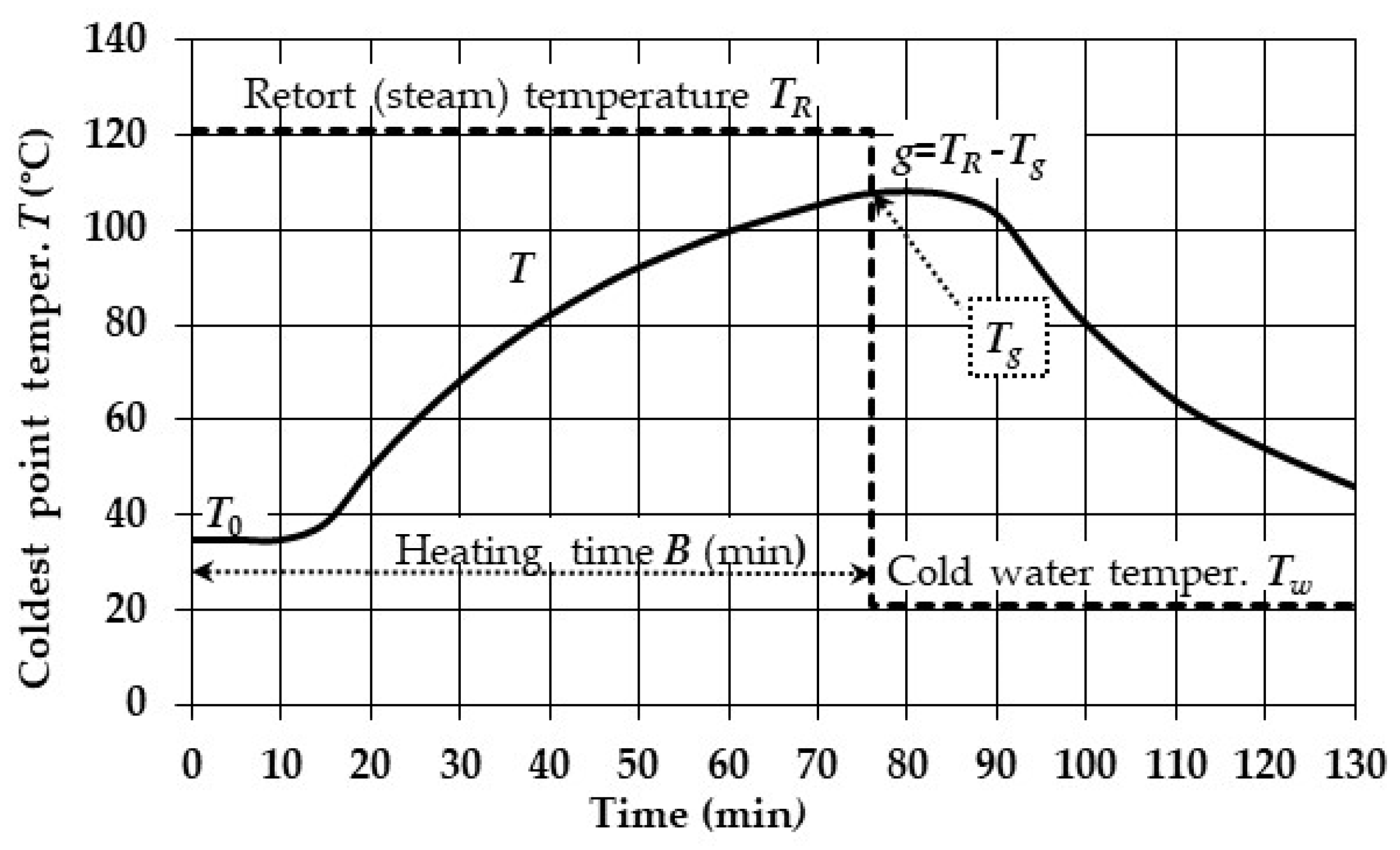
2.1.5. Exponential Decay–Heating Curve

To obtain the temperature–time relationship during the heating period (heating curve), Ball [9,10] considered that, after a possible initial lag, which had no influence on lethality, the temperature difference between the retort and the critical point $\left(T_R-T\right)$ (Figure 1) had an exponential decay with respect to time t:

$$(T_R-T)=(T_R-T_0)\cdot J_{ch}\cdot e^{{\displaystyle \frac{-2.303\cdot t}{f}}}$$

(12)

where T_R (°C) is the retort temperature, T₀ (°C) is the initial food temperature, J_ch is the lag factor and f (min) is the heating rate index, i.e., the time to reduce tenfold the temperature difference between the retort steam and the critical point of the canned food.

Highlighting the time t from Equation (12) and differentiating with respect to the temperature T, dt is

$$dt={\displaystyle \frac{f}{2.303}}·{\displaystyle \frac{dT}{T_R-T}}$$

(13)

Combining Equations (13) and (11), Ball [10] obtained the following:

$$F_h={\displaystyle \frac{f}{2.303}}{\int }_{44.4}^g{\displaystyle \frac{e^{2.303\frac{T-121.1}{z}}}{T_R-T}}dT$$

(14)

where $g=\left(T_R-T_g\right)$ is the difference between the retort temperature T_R and the canned food critical point temperature T_g at the end of the heating period (Figure 1); $\left(T_R-T\right)=44.4°\mathrm{C}$ is the lower integration limit, i.e., it is the initial temperature difference of the heating period that Ball [10] imposed equal to 44.4 °C (80 °F), a value that ensures the counting of all contributions to lethality; and F_h is the process lethality during the heating period.

Adding and subtracting the retort temperature T_R to the exponent, Equation (14) becomes

$$F_h=-{\displaystyle \frac{f}{2.303}}{e}^{2.303{\displaystyle \frac{T_R-121.1}{z}}}{\int }_{44.4}^g{\displaystyle \frac{e^{-2.303\frac{T_R-T}{z}}}{T_R-T}}d\left(T_R-T\right)$$

(15)

The integral of which is

$$U_h=F_h·e^{2.303{\displaystyle \frac{121.1{-T}_R}{z}}}=-{\displaystyle \frac{f}{2.303}}\left[\mathrm{Ei}\left({\displaystyle \frac{-2.303\cdot g}{z}}\right)-\mathrm{Ei}\left({\displaystyle \frac{-2.303\cdot 44.4}{z}}\right)\right]$$

(16)

where Ei is the exponential integral function. The expression $-\mathrm{E}\mathrm{i}\left(-x\right)$ appearing in Equation (16) is also indicated with the symbol ${\mathrm{E}}_1\left(x\right)$ [44]. Ball defined U_h as the sterilizing value. When the retort temperature T_R is equal to the reference temperature 121.1 °C (250 °F), the sterilizing value, U_h, coincides with the lethality F_h. If the retort temperature T_R is higher than 121.1 °C (250 °F), then $e^{2.303{\displaystyle \frac{121.1-T_R}{z}}}=10^{{\displaystyle \frac{121.1-T_R}{z}}}<1,$ and the time t_TR, i.e., the sterilizing value, $U_h=F_h\cdot 10^{{\displaystyle \frac{121.1-T_R}{z}}}$, is lower than the lethality F_h, meaning that the same result in terms of thermal death is now obtained by a time U_h shorter than F_h.

When the z value is less than 15 °C (26 °F), then $\mathrm{E}\mathrm{i}\left(-{\displaystyle \frac{2.303\cdot 44.4}{z}}\right)\to 0$. Therefore, Equation (16) simplifies to the following:

$$U_h=F_h·e^{2.303{\displaystyle \frac{121.1{-T}_R}{z}}}=-{\displaystyle \frac{f}{2.303}}\mathrm{Ei}\left({\displaystyle \frac{-2.303\cdot g}{z}}\right)$$

(17)

The Ei function is not an elementary function; its values must be obtained through an infinite series and are available in tables [43]. Ball [9,10] then used the tabulated values of Ei to produce his own tables with the data of some process parameters of his formula method.

2.1.6. Cooling Curve

The cooling curve starts at the steam-off point, which coincides with the cold-water-on point (Figure 1). Unlike the heating curve, which has a single temperature–time relationship, namely, Equation (12), the cooling curve requires two equations. The first one describes the temperature during the initial period, i.e., before the temperature difference between the critical point and the cold water $\left(T_R-T_W\right)$ undergoes an exponential decay vs. time t_c, and the second equation precisely describes this exponential decay. To describe the initial cooling curve, Ball, based on careful empirical evaluations, chose a hyperbola (Figure 2) that has the following equation of temperature T vs. time t_c, where t_c has its origin at the steam-off point:

$$T=T_g+a\left[1-\sqrt{1+{\displaystyle \frac{t_c^2}{b^2}}}\right]$$

(18)

where T_g is the critical point temperature of the canned food at the time of steam-off; the coefficient $a=0.3·m=0.3·\left(T_g-T_w\right)$; and the coefficient $b=0.175·f$. Ball established these two relationships about a and b under the assumption that the lag factor J_cc during cooling is constant and equal to 1.41 and that the cooling rate index f_c (min) is equal to the heating rate index: $f_c=f$. The index f_c is the time to decrease tenfold the temperature difference between the critical point of the canned food and the cold water.

Ball [9,10] established that the temperature value at the end of the initial cooling represented by Equation (18) is empirically $T_A=T_g-0.343·m=T_g-0.343·\left(T_g-T_w\right)$ (Figure 2). Ball then integrated the following to obtain the sterilizing value U_ic of this initial cooling:

$$U_{ic}=F_{ic}·e^{2.303{\displaystyle \frac{121.1{-T}_R}{z}}}={\displaystyle \frac{f}{2.303}}·e^{-2.303{\displaystyle \frac{g}{z}}}\left(0.332·e^{-0.789{\displaystyle \frac{m}{z}}}+0.253·{\displaystyle \frac{z}{m}}·e^{0.692{\displaystyle \frac{m}{z}}}·E\right)$$

(19)

The quantity E hides an integral that Ball had to calculate numerically and graphically [10]. This numerical/graphical calculation of E was an additional reason, alongside the one already reported with Equation (17), that forced Ball to prepare the tables that accompany the formula method.

When the temperature T_A is reached (Figure 2), cooling begins with the exponential decay of the temperature difference between the critical point and the cold water $\left(T-T_W\right)$. Like the exponential decay–heating curve (Section 2.1.5), Ball derived the equation that gives the sterilizing value of the exponential decay–cooling curve U_c:

$$U_c=F_c·e^{2.303{\displaystyle \frac{121.1{-T}_R}{z}}}={\displaystyle \frac{f}{2.303}}{e}^{-2.303{\displaystyle \frac{m+g}{z}}}\left[\mathrm{Ei}\left({\displaystyle \frac{2.303\cdot 0.657·m}{z}}\right)-\mathrm{Ei}\left({\displaystyle \frac{2.303\cdot \left(m+g-44.4\right)}{z}}\right)\right]$$

(20)

where (Figure 2) $m=T_g-T_w$ is equal to the difference between the critical point temperature T_g and the cold water temperature T_w; $g=T_R-T_g$ is equal to the difference between the retort temperature T_R and the critical point temperature T_g; and $m+g=T_R-T_w$ is equal to the difference between the retort temperature T_R and the cold water temperature T_w. The values of the exponential integral function of Equation (20) are also available in tabular form [43], so this is the third reason why Ball was forced to prepare his tables, which makes the original formula method non-computerizable.

2.1.7. Tables and Formula of Ball

The sum of the sterilizing values of Equations (17), (19) and (20) combined with some algebraic steps, gives

$${\displaystyle \frac{f}{U}}={\displaystyle \frac{f}{U_h+U_{ic}{+U}_c}}$$

(21)

Ball’s tables have a first row with the z values ranging from a minimum of 3.33 °C (6 °F) to a maximum of 15 °C (26 °F) and a first column on the left with the values of the f/U ratio. The range of values of this ratio are the result of the combination of the f and U that the canning industry adopts. The rest of the boxes in the tables are filled with the values of g that Ball calculated by solving Equation (21) for the implicit unknown g that appears within the three sterilizing values U_h, U_ic and U_c present in Equations (17), (19) and (20).

Ultimately, the formula method using Ball’s tables consists of determining the value of the required lethality F with Equation (9) starting from D_121,1 and n, known from thermo-bacteriology; calculating the sterilizing value U with the following $U=F·e^{2.303{\displaystyle \frac{121.1{-T}_R}{z}}}$; experimentally conducting a test to detect the values of the index f (Ball assumes that the cooling rate index f_c (min) is equal to the heating rate index $\left(f_c=f\right)$ and the cooling lag factor $J_{ch}=1.41$); calculating the ratio f/U; entering this value into Ball’s tables, together with the z value, known from thermo-bacteriology, and obtaining $g=\left(T_R-T_g\right)$; and finally, calculating the heating time B until steam-off, applying the following Formula derived from Equation (12):

$$B=f\cdot \log \left[{\displaystyle \frac{J_{ch}\left(T_R-T_0\right)}{g}}\right]$$

(22)

where log is the decimal logarithm.

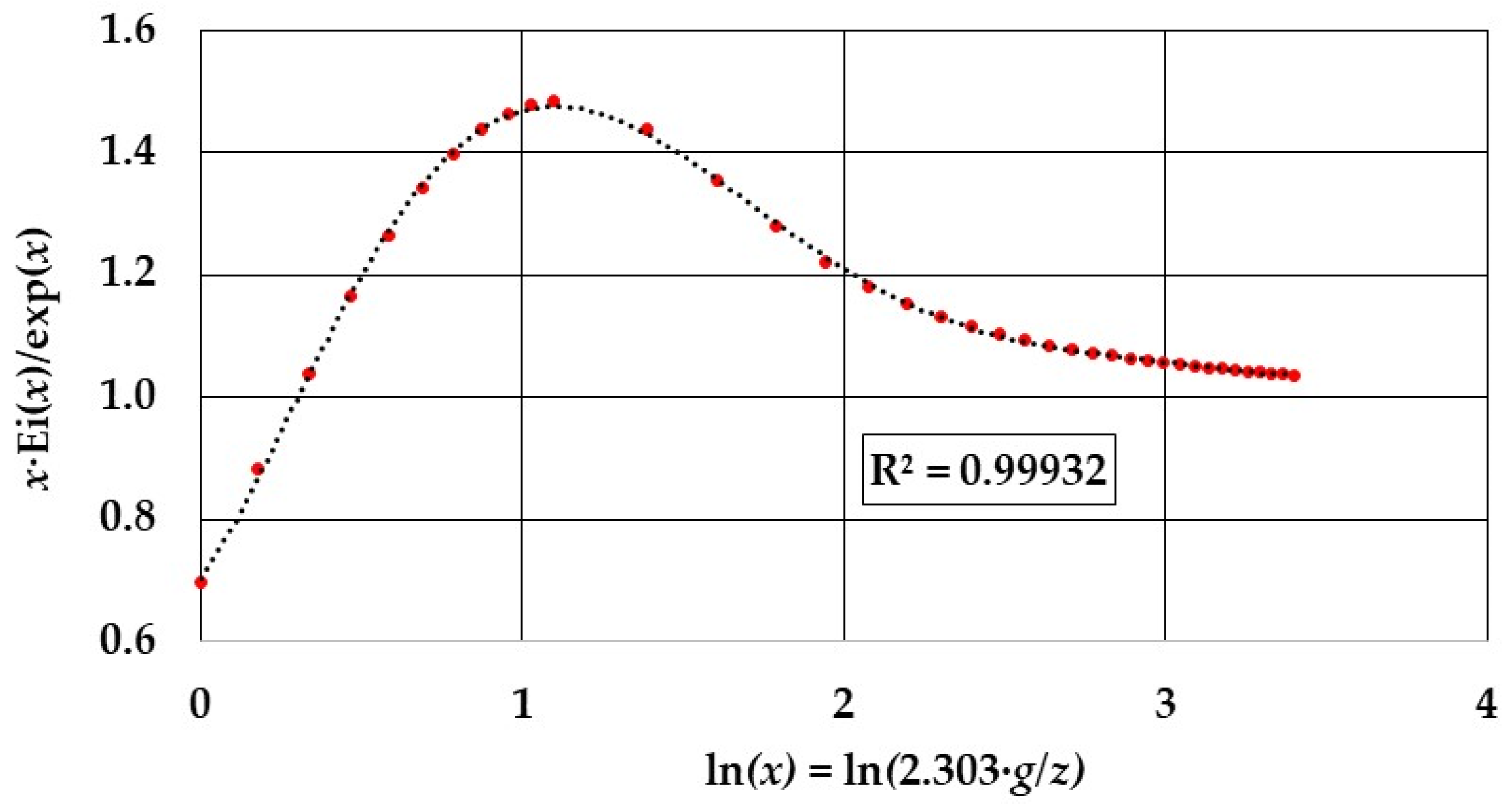
2.2. Development of an Analytical Approximation of the Exponential Integral Function Ei

Ball’s tables make computerization of the formula method impossible. As mentioned above, Ball’s tables are needed primarily because of the presence of the non-elementary exponential integral function Ei as a solution to the differential equation for lethality during the heating and cooling with temperature difference exponentially decaying. In fact, the Ei function requires to be represented by an infinite series. Using the nomenclature of Ball and Olson [10], the Ei function for the heating period can be described by the following series:

$$\mathrm{E}\mathrm{i}\left(-x\right)=0.5772+\ln \left(x\right)-x+{\displaystyle \frac{x^2}{2\cdot 2!}}-{\displaystyle \frac{x^3}{3\cdot 3!}}+......+{\displaystyle \frac{x^p}{p\cdot p!}}$$

(23)

The series can be truncated, thus introducing an approximation, which to be acceptable requires the presence of at least 40 terms in the equation resulting from the truncated series. Therefore, the use of such a long equation as an alternative to the tabulated values that Ball used is not at all easy. However, for values of x < 0.1, the series (23) truncated to the first three terms, $\mathrm{E}\mathrm{i}\left(-x\right)=0.5772+\ln \left(x\right)-x$, can represent the Ei function with an excellent approximation.

For the cooling period, the Ei function can instead be described by the following series:

$$\mathrm{E}\mathrm{i}\left(x\right)=0.5772+\ln \left(x\right)+x+{\displaystyle \frac{x^2}{2\cdot 2!}}+{\displaystyle \frac{x^3}{3\cdot 3!}}+......+{\displaystyle \frac{x^p}{p\cdot p!}}$$

(24)

Also in this case, what was said to be valid for the series (23) and that for x < 0.4, the series (24) can be truncated at the third term, ensuring an excellent approximation of the Ei function: $\mathrm{E}\mathrm{i}\left(x\right)=0.5772+\ln \left(x\right)+x.$

By imposing approximations of the two Ei functions, described by the infinite series (23) and (24), such as to ensure an average error of about 0.1%, the first possibility is the truncation to at least 40 terms of the same series. As already said above, these are final equations that are not at all easy. Therefore, equations with few terms of elementary functions that can represent Ei functions must be developed.

Table 1. Exact values of exponential integral function $\mathrm{E}\mathrm{i}\left(-x\right)$ vs. the x values.

x	Ei(−x)
0.11	−1.6974
1.15	−0.1716
3.22	−0.009882
6.21	−0.0002831
9.20	−0.000009988
12.19	−0.0000003872
15.18	−0.00000001584
18.17	−0.0000000006719
21.16	−0.00000000002921
24.15	−0.000000000001294
27.14	−0.00000000000005814
30.13	−0.000000000000002642

shows the exact values of $\mathrm{E}\mathrm{i}\left(-x\right)$ that vary rapidly in proximity to the zero of x and then vary less and less as x increases. This trend justifies the need to maintain at least the first 40 terms in the series (23) to have an acceptable approximation. Observing the variations in the values of $\mathrm{E}\mathrm{i}\left(-x\right)$ makes it clear that the absolute value of the derivative of the function also has a trend that first decreases rapidly and then more smoothly. Therefore, the ratio of the function with its derivative should have a much smoother trend with respect to x.

Consequently, it should be easier to approximate, via polynomial regression with a few terms, the ratio of the $\mathrm{E}\mathrm{i}\left(-x\right)$ function to its derivative rather than the function alone. This is also true for other functions, for example, the ratio of a polynomial to its derivative is a linear function. Another example is provided by the ratio of the exponential function to its derivative, which is the trivial function y = 1. Furthermore, the derivative of the $\mathrm{E}\mathrm{i}\left(-x\right)$ and $\mathrm{E}\mathrm{i}\left(x\right)$ functions has a very easy representation since it is the multiplication of two elementary functions, the exponential and the equilateral hyperbola: $d\mathrm{E}\mathrm{i}\left(-x\right)/dx=e^{-x}·\left(-1/x\right)$ and $d\mathrm{E}\mathrm{i}\left(x\right)/dx=e^x·\left(1/x\right).$

Therefore, with the exact values of the two functions, Ei(-x) and Ei(x), found in the tables [43] or downloaded from [48], and with the values of their respective derivatives, the two diagrams of the ratio $-x·\mathrm{E}\mathrm{i}(-x)/e^{-x}$ and $x·\mathrm{E}\mathrm{i}\left(x\right)/e^x$ vs. $\mathrm{l}\mathrm{n}\left(x\right)$ were plotted (Figure 3 and Figure 4). The choice to plot the ratio of the Ei function and its derivative vs. $\mathrm{l}\mathrm{n}\left(x\right)$ instead of x is due to the greater smoothness of the curve and therefore to the greater precision obtained with the subsequent polynomial regression.

The regression (R² = 0.99999) of the values of the ratio $-x·\mathrm{E}\mathrm{i}(-x)/e^{-x}$ in Figure 3 produced a 5° polynomial, which is presented inside the square brackets of Equation (25). Therefore, the exponential integral function $\mathrm{E}\mathrm{i}(-x)$ can be highlighted:

$$\mathrm{E}\mathrm{i}\left(-x\right)={\displaystyle \frac{e^{-x}}{-x}}\left[0.000013244·{\mathrm{l}\mathrm{n}}^{5}x+0.00049412{·\mathrm{l}\mathrm{n}}^{4}x-0.0072926·{\mathrm{l}\mathrm{n}}^{3}x-0.098067·{\mathrm{l}\mathrm{n}}^{2}x+0.18998·\ln x+0.59713\right]$$

(25)

This is valid for $0.09\le x\le 30$. Equation (25) provides negative values because the polynomial in the square brackets representing the curve in Figure 3 provides positive values, the e^−x function is positive, and the negative sign remains in front of x in the denominator. The relative mean error is MRE = 0.05% and the standard deviation SD = 0.03%. For $x<0.09$, the series (23) truncated at the third term can be used:

$$\mathrm{E}\mathrm{i}\left(-x\right)=0.5772+\ln \left(x\right)-x$$

(26)

The regression (R² = 0.99932) of the values of the ratio$x·\mathrm{E}\mathrm{i}\left(x\right)/e^x$ in Figure 4 gave a 6° polynomial, which is presented inside the square brackets of Equation (27). Therefore, the $\mathrm{E}\mathrm{i}\left(x\right)$ function can be highlighted:

$$\mathrm{E}\mathrm{i}\left(x\right)={\displaystyle \frac{e^x}{x}}\left[0.0235·{\mathrm{l}\mathrm{n}}^{6}x-0.2827·{\mathrm{l}\mathrm{n}}^{5}x+1.2663{·\mathrm{l}\mathrm{n}}^{4}x-2.4567·{\mathrm{l}\mathrm{n}}^{3}x+1.5081·{\mathrm{l}\mathrm{n}}^{2}x+0.7056·\ln x+0.7038\right]$$

(27)

This is valid for $1\le x\le 30$. The mean relative error is MRE = 0.79% and the standard deviation SD = 0.54%. For $x\le 1$, the series (24) truncated at the fourth term can be used:

$$\mathrm{E}\mathrm{i}\left(x\right)=0.5772+\ln \left(x\right)+x+{\displaystyle \frac{x^2}{4}}$$

(28)

2.3. The Formula Method in Combination with the Analytical Approximation of the Ei Function

2.3.1. Heating Curve

It is sufficient to insert into Equation (17) the polynomial (25) or (26) depending on the value of $x={\displaystyle \frac{2.303·g}{z}}$.

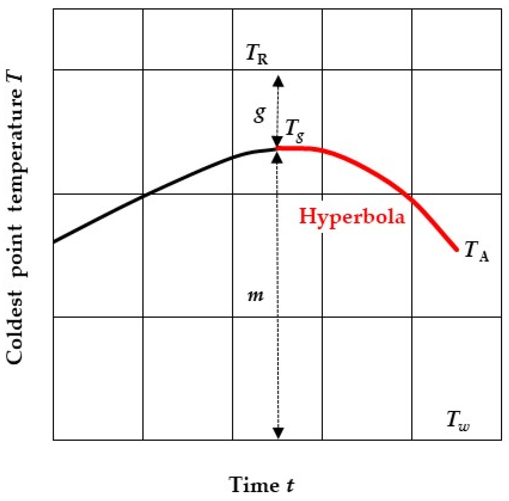
2.3.2. Initial Cooling Curve

This is the cooling from the point at temperature T_g (steam-off) (Figure 2) to the point at temperature T_A. This initial cooling corresponds to the lag portion of the cooling curve that Ball approximated with the hyperbola. Difficulties in solving the integral (19) analytically led Ball to perform numerical and graphical calculations and then to tabulate the results. To overcome this impossibility of a closed solution of Equation (19), in this work Ball’s hyperbola has been replaced by a portion of an exponential function such as the following:

$$T=T_g+k\left(1-e^{{\displaystyle \frac{2.303·t_c}{f}}}\right)$$

(29)

where t_c (min) is the cooling time with the origin at the cold-water-on (and steam-off); T_g is the temperature of the critical point (coldest point of the canned food) at the steam-off; and k is determined by the condition (Figure 2) that when $t_c=t_{cA}$, then $T=T_A$. Therefore, from Equation (29), the quantity k is as follows:

$$k={\displaystyle \frac{\left(T_A-T_g\right)}{\left(1-e^{\frac{2.303·t_{cA}}{f}}\right)}}$$

(30)

During the subsequent cooling, starting from the point at temperature T_A (Figure 2) where the temperature difference $T-T_w$ begins to follow the asymptotic decay law, the critical point temperature follows an equation like (12), which at point A appears as follows:

$$(T_A{-T}_w)=(T_g-T_w)\cdot J_{cc}\cdot e^{{\displaystyle \frac{-2.303\cdot t_{cA}}{f}}}$$

(31)

where the lag factor of the cooling curve, J_cc, was established by Ball to be 1.41. Combining the two Equations (30) and (31), considering that $m=\left(T_g-T_w\right),$ $\left(T_g-T_A\right)=0.343m,$ $\left(T_A-T_w\right)=0.657m,$ the quantity k becomes equal to coefficient a of Ball’s hyperbola (18):

$$k={\displaystyle \frac{\left(T_A-T_g\right)·\left(T_A{-T}_w\right)}{\left(T_A{-T}_w\right)-(T_g-T_w)\cdot J_{cc}}}=0.3·m=a$$

(32)

Isolating the time t_c from Equation (29), with k = a = 0.3·m, and differentiating, the differential dt_c is as follows:

$$d{t}_c=-{\displaystyle \frac{f}{2.303}}·{\displaystyle \frac{dT}{{0.3m+T}_g-T}}$$

(33)

Combining Equations (11) and (33), the process lethality during initial cooling F_ic is as follows:

$$F_{ic}=-{\displaystyle \frac{f}{2.303}}{\int }_{T_g}^{T_A}{\displaystyle \frac{e^{2.303\frac{T-121.1}{z}}}{{0.3m+T}_g-T}}dT$$

(34)

By adding and subtracting the sum $0.3m+T_g$ in the exponent and performing some algebraic transformations, Equation (34) becomes the following:

$$F_{ic}=-{\displaystyle \frac{f}{2.303}}{e}^{-2.303{\displaystyle \frac{121.1-0.3m-T_g}{z}}}{\int }_{T_A}^{T_g}{\displaystyle \frac{e^{-2.303\frac{0.3m+T_g-T}{z}}}{{0.3m+T}_g-T}}d\left({0.3m+T}_g-T\right)$$

(35)

The integral of this is

$$U_{ic}=F_{ic}·e^{2.303{\displaystyle \frac{121.1{-T}_R}{z}}}=-{\displaystyle \frac{f}{2.303}}{e}^{-2.303{\displaystyle \frac{T_R{-0.3m-T}_g}{z}}}\left[\mathrm{Ei}\left({\displaystyle \frac{-2.303\cdot 0.3m}{z}}\right)-\mathrm{Ei}\left({\displaystyle \frac{-2.303\cdot \left(0.3m+T_g-T_A\right)}{z}}\right)\right]$$

(36)

The sterilizing value U_ic obtained with Equation (36) is lower than that obtained by Ball with Equation (19) due to the slightly lower exponential curve compared to Ball’s hyperbola. Therefore, the coefficient k in Equation (29), equal to Ball’s coefficient $a=0.3·m$ as given in Equation (32), must be reduced by dividing it by a coefficient $\alpha \ge 1$ that depends on z, g and m. The relationship, $\alpha =\alpha \left(g,m,z\right)$, was found with a nonlinear multiple regression that minimizes the errors between the modelling results and the data from Ball’s tables:

$$\alpha =-0.0494·{\mathrm{l}\mathrm{n}}^2{\displaystyle \frac{g}{z}}-0.193·\mathrm{l}\mathrm{n}{\displaystyle \frac{g}{z}}+0.096·{\left({\displaystyle \frac{m+g}{{\left(m+g\right)}_{ref}}}\right)}^{-1}{\mathrm{l}\mathrm{n}}^2{\displaystyle \frac{m+g}{z}}+0.84{\left({\displaystyle \frac{m+g}{{\left(m+g\right)}_{ref}}}\right)}^{0.3}$$

(37)

where ${\left(m+g\right)}_{ref}$ is equal to 180 °F if all the other quantities present (g, m and z) are in °F. Otherwise, if g, m and z are in °C, then ${\left(m+g\right)}_{ref}=100°\mathrm{C}$.

Ultimately, also remembering that $T_g-T_A=0.343·m$ and $T_R-T_g=g,$ Equation (36) becomes

$$U_{ic}=F_{ic}·e^{2.303{\displaystyle \frac{121.1{-T}_R}{z}}}=-{\displaystyle \frac{f}{2.303}}{e}^{-2.303{\displaystyle \frac{g-0.3m/\alpha }{z}}}\left[\mathrm{Ei}\left(-2.303{\displaystyle \frac{0.3m/\alpha }{z}}\right)-\mathrm{Ei}\left(-2.303{\displaystyle \frac{0.3m/\alpha +0.343m}{z}}\right)\right]$$

(38)

Now, it is sufficient to insert into Equation (38) the polynomial (25) or (26) depending on the values of $x={\displaystyle \frac{2.303·0.3m/\alpha }{z}}$ and, respectively, $x={\displaystyle \frac{2.303·\left(0.3m/\alpha +0.343m\right)}{z}}$.

2.3.3. Exponential Decay–Cooling Curve

It is sufficient to insert the polynomial (27) twice into Equation (20), first with $x={\displaystyle \frac{2.303\cdot 0.657·m}{z}}$ and then with $x={\displaystyle \frac{2.303·\left(m+g-44.4\right)}{z}}$.

The temperature of 44.4 °C corresponds to 80 °F; therefore, the number 44.4 is fine if all the temperatures, m, g and z, in the equation are in °C, but if 80 is used then all the temperatures, m, g and z, must be in °F.

2.4. The Proposed Mathematical Modelling and Stoforos’ Modelling for a Comparison

2.4.1. Recap of the Proposed Mathematical Modelling

In place of reading Ball’s tables to obtain f/U with respect to g and z and the need to interpolate the data contained therein, the following mathematical modelling, just developed, can be used. It consists of Equation (21) in which the values of U_h, U_ic and U_c obtained, respectively, from the three Equations (17), (38) and (20) must be inserted.

For the sterilizing value U_h, the Equation (17) requires the value of the function $\mathrm{Ei}\left(-x\right)=\mathrm{Ei}\left({\displaystyle \frac{-2.303\cdot g}{z}}\right)$ obtained from the Equation (25) if $0.09\le \left(x={\displaystyle \frac{2.303\cdot g}{z}}\right)\le 30$. If $\left(x={\displaystyle \frac{2.303\cdot g}{z}}\right)<0.09$, then the $\mathrm{Ei}\left(-x\right)=\mathrm{Ei}\left({\displaystyle \frac{-2.303\cdot g}{z}}\right)$ value is obtained from the Equation (26).

For the sterilizing value U_c, the Equation (20) requires that the value of the function $\mathrm{E}\mathrm{i}\left(x\right)$ obtained from the Equation (27) must be inserted twice, first with $x={\displaystyle \frac{2.303\cdot 0.657·m}{z}}$ and then with $x={\displaystyle \frac{2.303\cdot \left(m+g-44.4\right)}{\mathrm{z}}}$.

For the sterilizing value U_ic, the Equation (38) requires that the value of the $\mathrm{E}\mathrm{i}\left(-x\right)$ obtained from the Equation (25) must be inserted twice, first with $x={\displaystyle \frac{2.303\cdot 0.3m/\alpha }{z}}$ and then with $x={\displaystyle \frac{2.303\cdot \left(0.3m/\alpha +0.343m\right)}{\mathrm{z}}}$.

The α value that must be inserted in Equation (38) can be calculated with Equation (37).

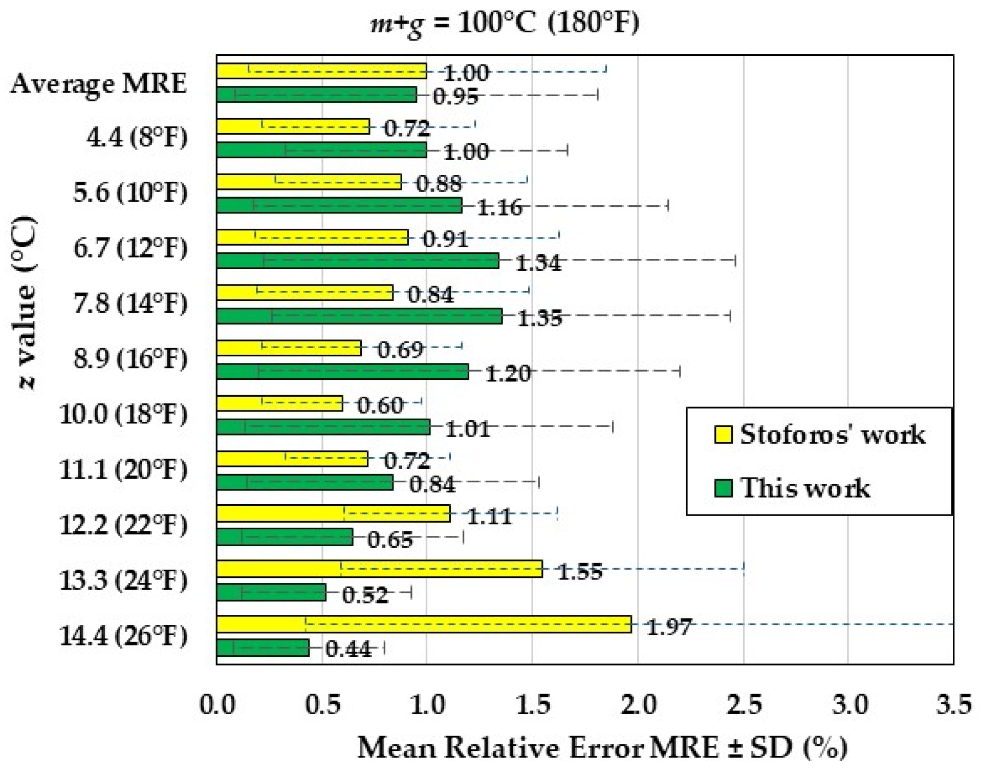
2.4.2. Stoforos’ Modelling and the Comparison Between the Two Models

To evaluate the results obtained by applying the modelling just proposed in Section 2.4.1, Stoforos’ modelling [44] was taken as a benchmark, which is the most accurate and recent available in the literature. It consists of an algebraic equation resulting from a nonlinear regression made directly on the pairs of values (g, f/U) as the z value varies:

$${\displaystyle \frac{f}{U}}=-{\displaystyle \frac{a_1}{1+a_2·e^{-a_3\left(\mathrm{l}\mathrm{o}\mathrm{g}(g/z-z/z_c\right)}}}+{\displaystyle \frac{a_4}{1+a_5·e^{-a_6\left(\mathrm{l}\mathrm{o}\mathrm{g}(g/z-z/z_c\right)}}}+a_7$$

(39)

where the eight numerical constants a₁ to a₇ and z_c have values that depend on m+g. Stoforos provided two sets of values for the eight constants, one for m+g of 100 °C (180 °F) and the other for m+g of 72.2 °C (130 °F), noting that, for intermediate values of m+g, linear interpolation is necessary. Alternatively, Stoforos suggested using only the algebraic equation with the coefficients for m+g = 100 °C (180 °F), introducing approximations that, on the one hand, favour microbiological safety and, on the other, produce over-sterilization.

Ball’s tables present f/U data down to a minimum g of 0.055 °C (0.1 °F). Ball also suggested that for g < 0.055 °C (g < 0.1 °F), the corresponding f/U value should be calculated with the following relationship, also used by Stoforos in his mathematical modelling, where z and g are expressed in °F:

$${\displaystyle \frac{f}{U}}={\displaystyle \frac{{10}^{\frac{0.1}{z}}·{\left(\frac{f}{U}\right)}_{g=0.1°F}}{{10}^{\frac{0.1}{z}}-\left[1+\mathrm{l}\mathrm{o}\mathrm{g}\left(g\right)\right]·{\left(\frac{f}{U}\right)}_{g=0.1°F}}}$$

(40)

Instead, the mathematical modelling proposed in this work does not require different coefficients for m+g of 130 °F compared to 180 °F and does not require interpolations for values of m+g different from 180 or 130 °F because Equations (17), (20), (21), (25), (27), (37) and (38) are valid for any value of m+g.

Furthermore, for values of g < 0.1 °F, the same equations maintain their ability to calculate the value of f/U up to g = 10⁻⁸ °F with a maximum relative error vs. Ball’s relationship (39) equal to 1.5%. It is only necessary not to use Equation (37) that provides the coefficient α because, with g < 0.1 °F, α is simply equal to 1.

Finally, Equations (17), (20), (21), (25), (27), (37) and (38) of the mathematical modelling can be used indifferently, with all the temperature differences present in the equations, i.e., $g=\left(T_R-T_g\right)$, $m=\left(T_g-T_w\right)$ and the z value, in °C, or with all the temperature differences and z value in °F.

3. Results and Discussion

Equations (17), (20), (21), (25), (27), (37) and (38) of the mathematical modelling were used to calculate the values of f/U by inserting the values of g read on two of Ball’s tables, the first for m+g = 100 °C (180 °F) and the second for m+g = 72.2 °C (130 °F). From both tables all the z values were considered, excluding the z value equal to 3.3 °C (6 °F) because this value was excluded by Stumbo [11] as unlikely in practice. For each z value (from 26 °F up to 8 °F), the rows of the tables involved in the comparison were 38 out of a total of 53 on average. The choice included all the rows from 20 up to 500 of the f/U values, while for an f/U between 0.6 and 17.5, 15 rows were alternately excluded because they were considered non-essential. The total number of data points was therefore 375 for each of the two tables and therefore for each of the two values of m+g.

The values of f/U obtained from the equations of this work were compared with those of Ball’s tables to obtain the mean relative error $\mathrm{M}\mathrm{R}\mathrm{E}={\displaystyle \frac{{\left(f/U\right)}_{calc}-{\left(f/U\right)}_{Ball}}{{\left(f/U\right)}_{Ball}}}·100$ and the standard deviation SD (%) for each z value.

Stoforos’ mathematical modelling was also used to calculate the f/U values and to calculate, vs. Ball’s tables, the MRE and SD values, with the same m+g values, the same z values and the same data points.

The MRE values for m+g = 100 °C (180 °F) of both this work and Stoforos’ work are shown in Figure 5. The maximum MRE occurs for z = 7.8 °C (14 °F) with a value of 1.35% ± 1.09%, while for Stoforos’ equations the maximum MRE occurs for z = 14.4 °C (26 °F) with a value of 1.97% ± 1.55%. The average MRE, calculated for all the z values, was 0.95% ± 0.86%, while for Stoforos’ equations the average MRE was 1.00% ± 0.85%. Therefore, the average MRE of the two modellings have almost equal values.

The MRE values for m+g = 72.2 °C (130 °F) of both this work and Stoforos’ work are shown in Figure 6. The maximum MRE occurs for z = 4.4 °C (8 °F) with a value of 1.24% ± 1.08%, while for Stoforos’ equations the maximum MRE occurs for z = 14.4 °C (26 °F) with a value of 1.50% ± 1.16%. The average MRE, calculated for all the z values, was 0.96% ± 0.78%, while for Stoforos’ equations the average MRE was 1.07% ± 0.80%. Therefore, also for m+g = 72.2 °C (130 °F), the average MREs of the two modellings have almost equal values.

For further information, the same f/U values, for all the z values predicted by the mathematical modelling of this work, were compared with those of Ball’s tables in Figure 7 and Figure 8 for m+g of 100 °C (180 °F) and 72.2 °C (130 °F), respectively. The two diagrams also present, in addition to the data, the regression line with an R² of 0.9998 and 0.9996, respectively, values that confirm the high accuracy of this mathematical modelling.

The f/U values predicted by Stoforos’ mathematical modelling were also compared with those of Ball’s tables in Figure 9 and Figure 10, respectively, for m+g of 100 °C (180 °F) and 72.2 °C (130 °F). In this case the regression line produced an R² of 0.9993 and 0.9997, respectively, values very similar to those in Figure 7 and Figure 8, which also confirm the high accuracy of Stoforos’ modelling.

In summary, the differences in the results of the f/U calculation between this mathematical modelling and Stoforos’ one are minimal, with a slight increase in accuracy in favour of the one proposed here. Stoforos’ one only involves two Equations (39) and (40), so his method of calculating f/U is easier.

The equations of the method proposed here are more numerous and therefore the algorithm is more laborious, but they are of a general nature. They do not require new values of the constants when the value of g+m is changed and when g < 10⁻¹ °F. In fact, they are valid for g up to 10⁻⁸ °F. It was the nonlinear regression of the exponential integral function and not the regression of the data from the Ball tables that made the equations in this work general in nature. For this same reason, the equations could also be used to simulate Stumbo’s tables [11] where z extends up to the value of 100 °C (180 °F), probably by modifying only Equation (37).

4. Conclusions

To overcome the long and tedious procedure of calculating food thermal processes provided by the general method, the so-called formula methods were established in the second half of the last century.

Furthermore, in the last 20 years studies have been carried out to use computational thermo-fluid dynamics (CFD). This approach seemed interesting, but it requires high computing power, long calculation times and considerable experience in the use of CFD that food technologists working in the canning industry do not have. The use of CFD also requires accurate knowledge of multiple data, such as the food thermal diffusivity, the convective heat transfer coefficient during the heating and cooling, etc.

Therefore, the formula methods are still very current. Among these, Ball’s original remains the most used for its accuracy and safety. However, the original Ball’s formula method requires consulting the tables prepared by Ball. This is primarily due to Ball’s choice to represent the initial cooling curve with the hyperbola. In fact, this choice made the analytical solution of the differential equation impossible. Secondly, during the heating and final cooling, which have an exponential decay law, the analytical solution presents the exponential integral function, which, being non-elementary, is available in an exact way only with the relevant tables.

Mathematical modelling that replaces Ball’s tables would be of great use, speeding up the calculation of the thermal process and providing a mathematical basis for the automation of process control. Several proposals have been made in this direction, among which Stoforos’ one stands out for its accuracy and simplicity. It is based on an algebraic equation obtained directly from the data of the tables with regression/optimization methods. The algebraic equation must be completed by knowing the values of the eight numerical coefficients it contains. Unfortunately, these coefficient values are not constant but depend on the difference in temperature of the steam for heating T_R and that of the water for cooling T_w: $m+g=\left(T_R-T_w\right)$.

Therefore, Stoforos provided two sets of values of the eight coefficients, one for m+g of 100 °C (180 °F) and the other for m+g of 72.2 °C (130 °F), pointing out that for intermediate values of m+g it is necessary to proceed with linear interpolations. Alternatively, Stoforos suggested using only the algebraic equation with the coefficients for m+g = 100 °C (180 °F), introducing approximations that, on the one hand, favour microbiological safety and, on the other, produce over sterilization.

To overcome these limitations, in this work, the mathematical modelling of Ball’s tables was found with a different approach. Instead of finding the regression equations from the data of Ball’s tables, the integration procedure of the three differential equations for the process lethality F was retraced, one for each of the three periods (Figure 1): (1) heating with an asymptotic decrease in the temperature difference; (2) initial cooling; and (3) cooling with an asymptotic decrease in the temperature difference.

The first step was to develop an analytical approximation of the exponential integral function Ei by obtaining two polynomial equations, one for positive values and one for negative values of the Ei function domain, which presented only elementary functions (logarithmic function and exponential function). The second step was to replace the hyperbola of the initial cooling adopted by Ball, with an appropriate exponential function. In this way, the result of the integration of the process lethality equation contained the exponential integral function similarly to what happens in heating and cooling with asymptotic decay.

The resulting set of equations allowed for the calculation of the process lethality F, followed by the sterilizing value U and finally the dimensionless ratio f/U. The values of this ratio were compared with those of the two Ball tables. For the first table relating to m+g = 100 °C (180 °F), the mean relative error and the standard deviation MRE ± SD was 0.95% ± 0.86%, and for the second table relating to m+g = 72.2 °C (130 °F), the MRE ± SD was 0.96% ± 0.78%. Similarly, it was performed using the equations proposed by Stoforos, obtaining, respectively, MRE ± SD = 1.00% ± 0.85% for m+g = 100 °C and MRE ± SD = 1.07% ± 0.80% for m+g = 72.2 °C. Therefore, the mean relative errors were almost equal with a slight improvement achieved by the equations of this work.

In terms of ease of calculation, Stoforos’ method is better because it has fewer equations. However, the greatest number of equations of the new modelling have a more general character because they are the result of nonlinear regressions of the exponential integral function and not of the data tabulated by Ball. That is, they do not need new values of the coefficients when the conditions are changed, such as the value of m+g or when the quantity g should be less than 10⁻¹ °F.

Finally, the method of the formula with the Stumbo tables is also widely used in the canning industry. These Stumbo tables were obtained in a similar way to those of Ball but present values of z that extend up to 100 °C (180 °F). Therefore, as the equations of this work are usable for any value of m+g, they will also be usable for any value of z, unlike the mathematical models based on the data of Ball’s tables. Such extensions of the equations will be carried out in future work.

References

1. Featherstone, S. A review of developments in and challenges in thermal processing over the past 200 years—A tribute to Nicolas Appert. Food Res. Int. 2012, 47, 156–160. [Google Scholar] [CrossRef]
2. Mafart, P. Food engineering and predictive microbiology: On the necessity to combine biological and physical kinetics. Int. J. Food Microbiol. 2005, 100, 239–251. [Google Scholar] [CrossRef] [PubMed]
3. Bigelow, W.D.; Bohart, G.S.; Richardson, A.C.; Ball, C.O. Heat Penetration in Processing Canned Foods, Bulletin 16-L Res., 1st ed.; Laboratory National Canners Associated: Washington, DC, USA, 1920; pp. 1–128. [Google Scholar]
4. Ball, C.O. Mathematical Solution of Problems on Thermal Processing of Canned Food, Berkley: Publication Health, 1st ed.; University of California Publications in Public Health: Berkeley, CA, USA, 1928; pp. 15–245. [Google Scholar]
5. Schultz, O.T.; Olson, F.C. Thermal processing of canned foods in tin containers. III. Recent improvements in the General Method of thermal process calculation. A special coordinate paper and methods of converting initial retort temperature. J. Food Sci. 1940, 5, 399–407. [Google Scholar] [CrossRef]
6. Patashnik, M. A simplified procedure for thermal process evaluation. Food Technol. 1953, 7, 1–6. [Google Scholar]
7. Hayakawa, K.I. A procedure for calculating the sterilizing value of a thermal process. Food Technol. 1968, 22, 93–95. [Google Scholar]
8. Simpson, R.; Almonacid, S.; Teixeira, A.A. Bigelow’s General Method revisited: Development of a new calculation technique. J. Food Sci. 2003, 68, 1324–1333. [Google Scholar] [CrossRef]
9. Ball, C.O. Thermal Process Times for Canned Foods, Bulletin 37, 1st ed.; National research Council: Washington, DC, USA, 1923; pp. 1–76. [Google Scholar]
10. Ball, C.O.; Olson, F.C. Sterilization in Food Technology, 1st ed.; McGraw-Hill: New York, NY, USA, 1957; pp. 1–507. [Google Scholar]
11. Stumbo, C.R. Thermobacteriology in Food Processing, 2nd ed.; Academic Press: New York, NY, USA, 1973; pp. 1–329. [Google Scholar]
12. Hemdon, D.H.; Griffin, R.C., Jr.; Ball, C.O. Use of computer derived tables to calculate sterilizing processes for packaged foods. Food Technol. 1968, 22, 473–484. [Google Scholar]
13. Griffin, R.C., Jr.; Hemdon, D.H.; Ball, C.O. Use of computer derived tables to calculate sterilizing processes for packaged foods. 2. Application to broken line heating curves. Food Technol. 1969, 23, 519–524. [Google Scholar]
14. Griffin, R.C., Jr.; Hemdon, D.H.; Ball, C.O. Use of computer derived tables to calculate sterilizing processes for packaged foods 3. Application to cooling curves. Food Technol. 1971, 25, 134–143. [Google Scholar]
15. Hayakawa, K. Experimental formulas for accurate estimation of transient temperature of food and their application to thermal process evaluation. Food Technol. 1970, 24, 1407–1418. [Google Scholar]
16. Larkin, J.W. Use of a modified Ball’s formula method to evaluate aseptic processing of foods containing particulates. Food Technol. 1989, 43, 124–131. [Google Scholar]
17. Steele, R.J.; Board, P.W. Thermal process calculations using sterilizing ratios. J. Food Technol. 1979, 14, 227–235. [Google Scholar] [CrossRef]
18. Larkin, J.W.; Berry, R.B. Estimating cooling process lethality for different cooling j values. J. Food Sci. 1991, 56, 1063–1067. [Google Scholar] [CrossRef]
19. Smith, T.; Tung, M.A. Comparison of formula methods for calculating thermal process lethality. J. Food Sci. 1982, 47, 626–630. [Google Scholar] [CrossRef]
20. Kim, K.H.; Teixeira, A.A.; Bichier, J.; Tavares, J. STERILIMATE: Software for designing and evaluating thermal sterilization processes. In Proceedings of the American Society of Agricultural Engineers. Meeting (USA), Chicago, IL, USA, 15 December 1993. ASAE paper No 93–4051. [Google Scholar]
21. Noronha, J.; Hendrickx, M.; Van Loey, A.; Tobback, P. New semi-empirical approach to handle time-variable boundary conditions during sterilization of non-conductive heating foods. J. Food Eng. 1995, 24, 249–268. [Google Scholar] [CrossRef]
22. Teixeira, A.A.; Balaban, M.O.; Germer, S.P.M.; Sadahira, M.S.; Teixeira-Neto Vitali, R.O. Heat Transfer Model Performance in Simulation of Process Deviations. J. Food Sci. 1999, 64, 488–493. [Google Scholar] [CrossRef]
23. Holdsworth, D.; Simpson, R. Thermal Processing of Packaged Foods, 2nd ed.; Springer: Berlin/Heidelberg, Germany, 2016; pp. 1–516. [Google Scholar]
24. Miranda Zamora, W.R.; Sanchez Chero, M.J.; Sanchez Chero, J.A. Software for the Determination of the Time and the F Value in the Thermal Processing of Packaged Foods Using the Modified Ball Method. In Intelligent Human Systems Integration (IHSI 2020): Integrating People and Intelligent Systems; Ahram, T., Karwowski, W., Vergnano, A., Leali, F., Taiar, R., Eds.; Springer: Modena, Italy, 2020; Volume 1131, pp. 498–502. [Google Scholar] [CrossRef]
25. Cleland, A.C.; Robertson, G.L. Determination of thermal processes to ensure commercial sterility of foods in cans. In Developments in Food Preservation, 1st ed.; Thorne, S., Ed.; Elsevier Applied Science: London, UK, 1985; Volume 3, pp. 1–315. [Google Scholar]
26. Hayakawa, K.I. A critical review of mathematical procedures for determining proper heat sterilization processes. Food Technol. 1978, 32, 59–65. [Google Scholar]
27. Stoforos, N.G.; Noronha, J.; Hendrickx, M.; Tobback, P.A. Critical analysis of mathematical procedures for the evaluation and design of in-container thermal processes for foods. Crit. Rev. Food Sci. Nutr. 1997, 37, 411–441. [Google Scholar] [CrossRef]
28. Sojecka, A.A.; Drozd-Rzoska, A.; Rzoska, S.J. Food Preservation in the Industrial Revolution Epoch: Innovative High Pressure Processing (HPP, HPT) for the 21st-Century Sustainable Society. Foods 2024, 13, 3028. [Google Scholar] [CrossRef]
29. Ghani, A.G.A.; Farid, M.M. Using the computational fluid dynamics to analyze the thermal sterilization of solid-liquid food mixture in cans. Innov. Food Sci. Emerg. 2006, 7, 55–61. [Google Scholar] [CrossRef]
30. Augusto, P.E.D.; Cristianini, M. Numerical simulation of packed liquid food thermal process using computational fluid dynamics (CFD). Int. J. Food Eng. 2011, 7, 16. [Google Scholar] [CrossRef]
31. Erdogdu, F. Optimization in Food Engineering, 1st ed.; CRC Press: Boca Raton, FL, USA, 2008; pp. 585–594. [Google Scholar] [CrossRef]
32. Dimou, A.; Panagou, E.; Stoforos, N.G.; Yanniotis, S. Analysis of Thermal Processing of Table Olives Using Computational Fluid Dynamics. J. Food Sci. 2013, 78, 1695–1703. [Google Scholar] [CrossRef]
33. Park, H.W.; Yoon, W.B. Computational Fluid Dynamics (CFD) Modelling and Application for Sterilization of Foods: A Review. Processes 2018, 6, 62. [Google Scholar] [CrossRef]
34. Azar, A.B.; Ramezan, Y.; Khashehchi, M. Numerical simulation of conductive heat transfer in canned celery stew and retort program adjustment by computational fluid dynamics (CFD). Int. J. Food Eng. 2020, 16, 20190303. [Google Scholar] [CrossRef]
35. Soleymani Serami, M.; Ramezan, Y.; Khashehchi, M. CFD simulation and experimental validation of in-container thermal processing in Fesenjan stew. Food Sci. Nutr. 2021, 9, 1079–1087. [Google Scholar] [CrossRef]
36. Zhu, S.; Li, B.; Chen, G. Improving prediction of temperature profiles of packaged food during retort processing. J. Food Eng. 2022, 313, 110758. [Google Scholar] [CrossRef]
37. Fu, Z.; Liu, H.; Huang, L.; Duan, L.; Wang, Y.; Sun, X.; Zhou, C. Numerical simulation of thermal sterilization heating process of canned fruits with different shapes based on UDM and RDM. Int. J. Food Eng. 2023, 19, 159–175. [Google Scholar] [CrossRef]
38. Das, S.; Baro, R.K.; Kotecha, P.; Anandalakshmi, R. Numerical studies on thermal processing of solid, liquid, and solid–liquid food products: A comprehensive analysis. J. Food Process Eng. 2023, 46, e14484. [Google Scholar] [CrossRef]
39. Dalvi-Isfahan, M. Effect of flow behavior index of CMC solutions on heat transfer and fluid flow in a cylindrical can. J. Food Process Eng. 2024, 47, e14672. [Google Scholar] [CrossRef]
40. Sampanis, P.-A.; Chatzidakis, S.M.; Stoforos, G.N.; Stoforos, N.G. Analysis of Shell Egg Pasteurization Using Computational Fluid Dynamics. Appl. Sci. 2025, 15, 1263. [Google Scholar] [CrossRef]
41. Szpicer, A.; Bińkowska, W.; Stelmasiak, A.; Zalewska, M.; Wojtasik-Kalinowska, I.; Piwowarski, K.; Piepiórka-Stepuk, J.; Półtorak, A. Computational Fluid Dynamics Simulation of Thermal Processes in Food Technology and Their Applications in the Food Industry. Appl. Sci. 2025, 15, 424. [Google Scholar] [CrossRef]
42. Calomino, G.E.; Minim, L.A.; Coimbra, J.S.D.; Rodrigues Minim, V.P. Thermal process calculation using artificial neural networks and other traditional methods. J. Food Process Eng. 2006, 29, 162–173. [Google Scholar] [CrossRef]
43. Gautschi, W.; Cahill, W.F. Exponential integral and related functions. In Handbook of Mathematical Functions, 1st ed.; Abramowitz, M., Stegun, I.A., Eds.; National Bureau of Standards: Washington, DC, USA, 1964; Appl Math Ser; Volume 55, pp. 227–237. [Google Scholar]
44. Stoforos, N.G. Thermal process calculations through Ball’s original formula method: A critical presentation of the method and simplification of its use through regression equations. Food Eng. Rev. 2010, 2, 1–16. [Google Scholar] [CrossRef]
45. Friso, D. A new mathematical model for food thermal process prediction. Model. Simul. Eng. 2013, 2013, 1–8. [Google Scholar] [CrossRef]
46. Friso, D. A Mathematical Solution for Food Thermal Process Design. Appl. Math. Sci. 2015, 9, 255–270. [Google Scholar] [CrossRef]
47. Friso, D. The Check Problem of Food Thermal Processes: A Mathematical Solution. Appl. Math. Sci. 2015, 9, 6529–6546. [Google Scholar] [CrossRef]
48. Wolframalpha. Available online: https://www.wolframalpha.com (accessed on 20 April 2025).
Figure 1. Heat penetration curve or temperature–time history of the critical point (coldest point) of the canned food during the entire thermal process from the heating period to the cooling one.
Processes 13 01975 g001
Figure 2. Hyperbola approximating the lag portion of the cooling curve.
Processes 13 01975 g002
Figure 3. Ratio of the exponential integral function E i ( x )   to its derivative e x x , E i ( x ) / e x x vs. ln x = l n ( 2.303 · g z ) . The red dots are the ratio between the exact values of E i ( x ) , obtained from [48], and the derivative e x x ; the black dashed line is the 5° polynomial of the regression (R2 = 0.99999).
Processes 13 01975 g003
Figure 4. Ratio of the exponential integral function E i ( x )   to its derivative e x x , E i ( x ) / e x x vs. ln x = l n ( 2.303 · g z ) . The red dots are the ratio between the exact values of E i ( x ) , obtained from [48], and the derivative e x x ; the black dashed line is the 6° polynomial of the regression (R2 = 0.99932).
Processes 13 01975 g004
Figure 5. Percentage mean relative error MRE (coloured bars with numeric values) and percentage standard deviation SD (dashed lines) calculated by comparing the exact f/U values of Ball’s table (m+g = 100 °C = 180 °F) with those of the two mathematical models: this work and Stoforos’ work. The first double bar at the top gives the two average MRE ± SDs obtained by averaging the ten MREs corresponding to each z value.
Processes 13 01975 g005
Figure 6. Percentage mean relative error MRE (coloured bars with numeric values) and percentage standard deviation SD (dashed lines) calculated by comparing the exact f/U values of Ball’s table (m+g = 72.2 °C = 130 °F) with those of the two mathematical models: this work and Stoforos’ work. The first double bar at the top gives the two average MRE ± SDs obtained by averaging the ten MREs corresponding to each z value.
Processes 13 01975 g006
Figure 7. Predicted f/U values using the mathematical modelling of this work vs. the desired Ball’s values of f/U for m+g = 100 °C (180 °F).
Processes 13 01975 g007
Figure 8. Predicted f/U values using the mathematical modelling of this work vs. the desired Ball’s values of f/U for m+g = 72.2 °C (130 °F).
Processes 13 01975 g008
Figure 9. Predicted f/U values using the mathematical modelling of Stoforos’ work vs. the desired Ball’s values of f/U for m+g = 100 °C (180 °F).
Processes 13 01975 g009
Figure 10. Predicted f/U values using the mathematical modelling of Stoforos’ work vs. the desired Ball’s values of f/U for m+g = 72.2 °C (130 °F).
Processes 13 01975 g010