A New Method for Calculating Carbonate Mineral Content Based on the Fusion of Conventional and Special Logging Data—A Case Study of a Carbonate Reservoir in the M Oilfield in the Middle East

Abstract

In this study, we propose a self-adaptive weighted multi-mineral inversion model (SQP_AW) based on Sequential Quadratic Programming (SQP) and the Adam optimization algorithm for the accurate evaluation of mineral content in carbonate reservoir rocks, addressing the high costs of traditional experimental methods and the strong parameter dependence in geophysical inversion. The model integrates porosity curves (compensated density, compensated neutron, and acoustic time difference), elastic modulus parameters (shear and bulk moduli), and nuclear magnetic porosity data for the construction of a multi-dimensional linear equation system, with calibration coefficients derived from core X-ray diffraction (XRD) data. The Adam algorithm dynamically optimizes the weights, solving the overdetermined equation system. We applied the method to the Asmari Formation in the M oilfield in the Middle East with 40 core samples for calibration, achieving a 0.91 fit with the XRD data. For eight additional uncalibrated samples from Well A, the fit reaches 0.87. With the introduction of the elastic modulus and nuclear magnetic porosity, the average relative error in mineral content decreases from 9.45% to 6.59%, and that in porosity estimation decreases from 8.1% to 7.1%. The approach is also scalable to elemental logging data, yielding inversion precision comparable to that of commercial software. Although the method requires a complete set of logging data and further validation of regional applicability for weight parameters, in future research, transfer learning and missing curve prediction could be incorporated to enhance its practical utility.

1. Introduction

The precise calculation of reservoir mineral content is a key component in oil and gas reservoir exploration and development, effectively assisting in the classification of rock physics types and the accurate calculation of reservoir parameters [1,2]. This is particularly important in complex reservoirs with a wide variety of mineral types, where the detailed evaluation of mineral content lays a crucial data foundation for the subsequent determination of lithology and the delineation of flow units [3,4].

The methods for determining mineral content can primarily be categorized into experimental techniques and geophysical inversion methods [5]. In the case of experimental methods, core samples are analyzed by on-site geological experts to identify lithological types. However, this approach is highly dependent on the expert’s experience and does not allow one to accurately determine the specific mineral content [6]. Thin-section petrography can provide preliminary estimates of the mineral content in various lithologies, but its precision is limited. The most accurate method currently available is the use of X-ray diffraction (XRD) analysis on core samples, which can precisely quantify mineral content [7,8]. However, this technique has limitations: firstly, the availability of core samples is often limited, preventing its widespread application in all wells, and secondly, XRD analysis is costly, which further restricts its large-scale adoption. These constraints hinder the broader use of core sample-based methods in mineral content determination [9].

Geophysical logging methods are widely recognized for their high reliability and strong resolution, which makes them an essential tool in lithology and mineral content inversion. Among various geophysical logging data, elemental capture spectroscopy (ECS) logging is considered the most reliable technique for evaluating mineral content [10]. Since its development in the 1970s, ECS logging has been able to accurately quantify the primary chemical elements in formations, with broad applications in mineral composition analysis, lithology identification, and brittleness evaluation [1,11]. Current multi-mineral inversion methods based on formation element logging primarily include the oxide closure model method and optimization-based methods [12]. Extensive research has been conducted on these methods, and various findings indicate that while the oxide closure model method is straightforward and easy to implement, its results tend to be relatively coarse and fail to meet high-precision inversion requirements [13]. On the other hand, optimization methods can invert more mineral components with higher precision and have been widely applied in software tools such as Ciflog and Techlog [14]. However, these methods involve many parameters, such as conversion factors, uncertainty, and weight settings, all of which significantly affect the inversion results [15]. The applicability of default parameters is often uncertain when applied to reservoirs with different geological backgrounds. Given that many oil fields do not collect element logging data, the most commonly used method combines conventional logging data with multi-mineral inversion algorithms to estimate mineral content [16]. This approach essentially treats the problem as solving a system of linear equations. Various techniques have been introduced for solving such systems, such as linear programming, generalized inverse matrix methods, and linear weighted least squares, all of which effectively address the challenges in equation system solving [1,17,18]. However, these methods typically employ fixed weight coefficients, neglecting the potential impact of adjusting weight coefficients to improve inversion accuracy. With the advancement of data-driven methods, deep learning techniques have been widely applied in the field of mineral component inversion [19,20]. Models such as Convolutional Neural Networks (CNNs), Long Short-Term Memory (LSTM) networks, and Gated Recurrent Units (GRUs) are capable of capturing complex nonlinear relationships and spatiotemporal dependencies in logging data [21,22,23], significantly enhancing inversion accuracy. For instance, Tariq et al. [24] established a relationship model between rock mineral content and porosity by using Deep Neural Networks (DNNs), while Wang et al. [25] employed Deep Convolutional Neural Networks (DCNN). Wang et al. [26] adopted Spatiotemporal Neural Networks (STNNs), and Zhai et al. (2023) [27] introduced attention mechanisms, further enhancing the reconstruction and prediction capabilities of 2D Convolutional Neural Networks for logging curves. However, the application of these data-driven methods requires accurate core mineral content data as prediction features, which often depend on the availability of XRD experimental data. Due to the cost of coring and experiments, the quantity of such data is usually limited, which poses a constraint when applying these methods in practice [28].

In conclusion, the inversion of lithology mineral content requires a method that not only ensures the accuracy of mineral content calculations but also meets the practical needs of oilfield applications. In this study, we introduce an innovative approach based on conventional logging curves and parameters derived from specialized logging data, incorporating Sequential Quadratic Programming (SQP) combined with the Adam (Adaptive Moment Estimation) optimization algorithm to construct a model (SQP_AW) with adaptive weight parameters for mineral content inversion. The method was applied to the Asmari Formation in the M oilfield in the Middle East, and its results were compared with core mineral content data, showing a high degree of agreement. This approach significantly improves the accuracy of porosity estimation and addresses the limitations of traditional multi-mineral evaluation methods under complex geological conditions. The proposed method demonstrates considerable potential for practical applications and holds significant engineering value.

2. Geological Overview and Material Sources

2.1. Geological Overview

The study area is the M oilfield, located in the Middle East, spanning the southeastern part of Iraq and the southern border of Iran. The core of the reservoir is composed of the Paleogene Asmari Formation, which consists of carbonate rocks. In terms of structural location, the oilfield lies in the transitional structural zone between the northern Persian Gulf Basin and the Mesopotamian Basin, extending towards the foreland depression belt of the Zagros Mountains [29,30]. Its formation and evolution are directly influenced by the collision between the African–Arabian and Eurasian plates, triggering the Zagros orogeny [31].

In the M oilfield in the study area, the Cretaceous sequences, particularly the Asmari Formation, predominantly consist of limestone, mudstone, and sandstone, which together form key petroleum and natural gas reservoirs within the basin [32,33].

2.2. Material Source and Determination of Core Mineral Content

Core samples were collected with on-site drilling (Figure 1) and sent to the laboratory, where they were ground to the appropriate size for XRD analysis. Figure 2 shows the XRD results of the core samples. The specific data in Figure 2 facilitate the calculation of specific values of the content of each mineral in each core sample.

The mineral content in the core samples was determined by comparing the X-ray spectra with the D-values of each mineral (Figure 3). The mineral composition analysis revealed that the Asmari Formation in the study area contains five key minerals: gypsum, dolomite, calcite, quartz, and clay. Unlike the pure limestone of the Mishrif Formation, the Asmari Formation is primarily composed of carbonate rocks. However, the core sample data indicate a diverse range of minerals within this formation, highlighting the necessity for precise mineral content calculations. This study focuses on how to estimate the content of these five minerals by using geophysical well-logging data.

3. Methods and Principles

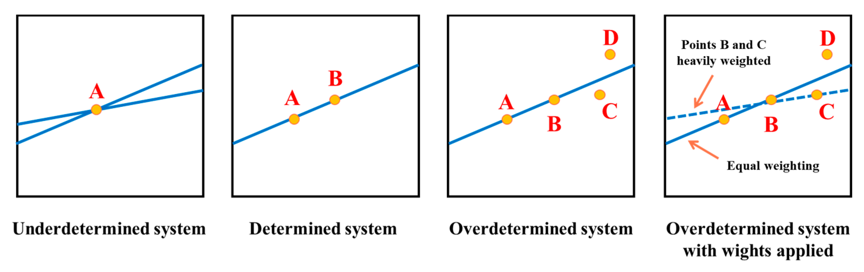
3.1. Construction of Linear Equations

The inversion of lithology and mineral content is essentially a process of solving linear equations. Taking a well with element logging data as an example, the conversion relationship between the dry weight of the elements and the mineral composition can be expressed in matrix form as shown in Equation (1):

$$\left[T\right]=\left[V\right]\times \left[R\right]$$

(1)

In Equation (1), [T] represents the element dry weight matrix, [V] represents the mineral dry weight matrix, and [R] is the coefficient matrix that converts the element dry weight into mineral composition content. Based on this relationship, a system of linear equations can be established as shown in Equation (2):

$$T_j={\displaystyle \sum _i^n{V}_i\times R_{ji}}$$

(2)

In Equation (2), $T_j$ represents the dry weight of the j-th element, calculated based on the corresponding mineral content. $V_i$ denotes the content of the i-th mineral, while $R_{ji}$ is the conversion factor between the i-th mineral and the j-th element. n is the total number of selected mineral types. A system of m linear equations can be formed, as expressed in Equation (3), by constructing linear equations for the dry weight of elements, with each corresponding to one of the m elements. This system, with dimensions of ($m\times n$), serves to solve for the mineral composition content [34].

$$\left\{\begin{array}{c}{T}_1={\displaystyle {\sum }_{i=1}^n{V}_i\times R_{1i}}\\ T_2={\displaystyle {\sum }_{i=1}^n{V}_i\times R_{2i}}\\ ⋮\\ T_m={\displaystyle {\sum }_{i=1}^n{V}_i\times R_{mi}}\end{array}\right.$$

(3)

At the same time, the mineral component content required by the equation set needs to meet the basic constraints shown in Equations (4) and (5):

$${\displaystyle {\sum }_{i=1}^n{V}_i}=1$$

(4)

$$0<V_i<1$$

(5)

Equation (4) indicates that the sum of the contents of all mineral components cannot exceed 100%, meaning that the total proportion of mineral components in the rock volume should be less than or equal to 1. Equation (5) stipulates that the content of each mineral component must be non-negative, i.e., the mineral content cannot be negative.

In practical applications, the cost of obtaining elemental logging data is high. Such methods can be substituted by conventional logging curves, such as density, neutron, and sonic, through linear inversion. The conventional approach involves using the natural gamma logging curve to calculate the clay content and then inverting the content of other minerals by using three porosity curves. However, the range of invertible mineral types is limited in this case. Kumar et al. [35] enriched the system of equations by introducing the shear modulus, $\mu =\rho \Delta t_s$, and the bulk modulus, $K=\rho \left(\Delta t_p^2-{\displaystyle \frac{4}{3}}\Delta t_s^2\right)$, from the elastic modulus to address this issue. Li et al. [36] introduced nuclear magnetic resonance porosity, ${\varphi }_{NMR}$, into the system of equations and demonstrated its feasibility in tight sandstone reservoirs. Considering that for the study area, conventional, array sonic, and nuclear magnetic resonance logging data have been collected, a system of linear equations is constructed by using the three conventional porosity curves, the shear modulus, the bulk modulus, and nuclear magnetic porosity, totaling six curves.

$$\left\{\begin{array}{c}{\rho }_b={\displaystyle {\sum }_{i=1}^n{V}_i\times {\rho }_i}\\ {\varphi }_N={\displaystyle {\sum }_{i=1}^n{V}_i\times {\varphi }_{Ni}}\\ \Delta t_p={\displaystyle {\sum }_{i=1}^n{V}_i\times \Delta t_{pi}}\\ \mu ={\displaystyle {\sum }_{i=1}^n{V}_i\times {\mu }_i}\\ K={\displaystyle {\sum }_{i=1}^n{V}_i\times K_i}\\ {\varphi }_{NMR}={\displaystyle {\sum }_{i=1}^n{V}_i\times {\varphi }_{NMRi}}\end{array}\right.$$

(6)

The inversion equations constructed with the compensation density (${\rho }_b$), the supplementary neutron (${\varphi }_N$), the longitudinal wave time difference ($\Delta t_p$), the shear modulus ($\mu$), the bulk modulus ($K$), and the nuclear magnetic porosity (${\varphi }_{NMR}$) are shown in Equation (6).

3.2. The Objective Function Based on the Principle of Linear Weighted Least Squares

When performing multi-mineral content inversion by using geophysical logging curves, the m × n dimensional linear system can be analyzed based on the number of equations (m) and the number of minerals (n) being solved for (Figure 4). The relationship between the number of equations and the mineral types can be classified into three cases. When m = n, the system is well conditioned with a unique solution. When m < n, the system is underdetermined, typically yielding infinitely many solutions. In this case, it is necessary to either add more equations or reduce the number of minerals. When m > n, the system becomes overdetermined and typically does not have an exact solution. In such cases, methods such as least squares, QR decomposition, LU decomposition, and singular value decomposition (SVD) can be applied to obtain an approximate solution.

In multi-mineral inversion, as the number of logging curves increases, the system typically encounters overdetermined equations. In the context of the study area, where inversion involves five mineral types, the number of curves exceeds the number of minerals to be inverted, meaning that the number of equations (m) is greater than the number of selected minerals (n). As a result, an exact solution does not exist, and optimization techniques are generally applied to find a solution. By integrating concepts such as the least squares principle and weighting factors, an objective function can be constructed as shown in Equation (7).

$$\min f\left(\overrightarrow{V}\right)={\displaystyle \sum _{j=1}^m{\left[\left(T_j-L_j\right)\times w_j\right]}^2}$$

(7)

In Equation (7), $T_j$ and $L_j$ represent the logging responses obtained from the inversion calculation of the j-th response equation and the actual responses measured with the instrument, respectively, while $w_j$ is the weight associated with the corresponding equation. Since different logging curves have varying impacts on the final result, the weight ($w_j$) serves to adjust the relative importance of each logging curve and can be expressed as

$$w_j={\displaystyle \frac{W{P}_j}{MaxWeight}}\times {\displaystyle \frac{1}{UN{C}_j}}$$

(8)

The role of the weight ($w_j$) is to adjust the relative importance of different logging curves, as the influence of each curve on the final result varies. In the weight formula (8), the uncertainty of the j-th logging curve is considered. Quirein [37] proposed that measurement errors can be quantified by using uncertainty, which allows the measurement values to be adjusted to dimensionless numbers, ensuring consistent amplitude variations across different logging curves. This uncertainty serves as an influence factor for the j-th logging curve, determined based on geological context and the quality of the logging curve. MaxWeight represents the maximum influence factor, which is manually defined across all logging curves to normalize the influence factors.

3.3. Improvement and Application of Sequential Quadratic Programming Method

3.3.1. Principle and Solving Steps of Sequential Quadratic Programming Method

When solving weighted and constrained problems by using the least squares principle, there are various optimization methods available. One such method is SQP, which is specifically designed to address nonlinear constrained optimization problems. The core idea of SQP is to convert the nonlinear optimization problem into a series of linear or quadratic programming subproblems, which are solved iteratively to progressively approximate the optimal solution. The detailed steps for solving the problem are as follows:

(1)

Define the objective function: Initially, the objective function and constraints of the nonlinear constrained optimization problem are mathematically modeled. The objective function can be nonlinear, while the constraints typically consist of both equality and inequality conditions.

(2)

Select an initial point: An initial point is chosen to start the optimization process. This point must generally satisfy the constraint conditions to ensure that the optimization procedure proceeds smoothly.

(3)

Linearize the objective function and constraints: Based on the current point, the objective function and constraints are linearized to formulate a linear programming subproblem.

(4)

Solve the linear subproblem: Linear programming solving techniques, such as interior-point methods or gradient projection methods, are employed to solve the linear subproblem and obtain a new iteration point.

(5)

Determine the step size: The step size from the current point to the new iteration point is computed, typically by using a one-dimensional search method (e.g., Armijo’s rule), ensuring that each iteration makes sufficient progress.

(6)

Update the current point: The current point is updated to the new iteration point, where the step size is denoted as $x_{k+1}\leftarrow x_k+{\alpha }_k·\Delta x_k$.

(7)

Check for convergence: Finally, the method checks whether the current point meets the convergence criteria, such as whether the change in the objective function is below a predefined threshold or the constraint conditions are satisfied. If the termination criteria are not met, the process returns to step 3 for further iterations until convergence is achieved.

In step 3, the Taylor expansion is often used to approximate the nonlinear functions as linear functions, resulting in linearized objective function and constraints, as shown in Equation (9):

$$f(x+\Delta x)\approx f(x)+\nabla f(x)·\Delta x+{\displaystyle \frac{1}{2}}\Delta x^T{\nabla }^{2}f(x)·\Delta x$$

(9)

In Equation (9), $\Delta x$ represents the increment in the optimization variables, $\nabla f(x)$ is the gradient of objective function $f(x)$, and ${\nabla }^{2}f(x)$ is the Hessian matrix of the objective function. The Hessian matrix is used to represent the second-order derivatives of the objective function and plays a crucial role in evaluating the curvature of the objective function during the optimization process.

For the constraint conditions, both the equality constraint function, $h_j(x)$, and the inequality constraint function, $g_i(x)$, can also be linearized:

$$\begin{array}{l}{h}_j(x+\Delta x)\approx h_j+\nabla h_j(x)·\Delta x\\ g_i(x+\Delta x)\approx g_i+\nabla g_i(x)·\Delta x\end{array}$$

(10)

In Equation (10), $\nabla h_j(x)$ is the gradient of the equality constraint function, $h_j(x)$, and $\nabla g_i(x)$ is the gradient of the inequality constraint function, $g_i(x)$.

3.3.2. Construction of SQP_AW Model

We present a mineral composition inversion model (SQP_AW) that combines SQP with the Adam optimization algorithm based on XRD data.

The Adam algorithm integrates the advantages of gradient descent and momentum optimization [38], enabling adaptive learning rate adjustments that accelerate convergence. By using exponential moving averages to estimate the first and second moments of the gradient, Adam adapts to the varying learning rate requirements of different parameters. Its strengths lie in its fast convergence in high-dimensional, non-convex, and sparse data scenarios. Compared with other adaptive learning rate algorithms, Adam is more efficient and has become one of the most widely used optimization algorithms in deep learning [39]. The update rule of the Adam algorithm consists of several steps, first-order momentum update, second-order momentum update, bias correction for the first and second moments, and final weight update, as detailed in Equations (11)–(15).

$$m_t={\beta }_1{m}_{t-1}+(1-{\beta }_1)g_t$$

(11)

$$v_t={\beta }_2{v}_{t-1}+(1-{\beta }_2)g_t^2$$

(12)

$${\widehat{m}}_t={\displaystyle \frac{m_t}{1-{\beta }_1^t}}$$

(13)

$${\widehat{v}}_t={\displaystyle \frac{v_t}{1-{\beta }_2^t}}$$

(14)

$$w_{t+1}=w_t-\alpha {\displaystyle \frac{{\widehat{m}}_t}{\sqrt{{\widehat{v}}_t+\epsilon }}}$$

(15)

In the above equations, $m_t$ is the first-order momentum of the gradient; $v_t$ is the second-order momentum of the gradient; ${\beta }_1$ and ${\beta }_2$ are the momentum and Root Mean Square Propagation (RMSProp) coefficients, respectively; $\alpha$ denotes the learning rates; $\epsilon$ denotes the small constants that prevent division by zero; $g_t$ is the current gradient; and ${\widehat{m}}_t$ and ${\widehat{v}}_t$ are the momentum and second-order momentum after deviation correction, respectively.

In this study, we construct an evaluation metric as shown in Equation (16) based on the mineral composition inversion results, XRD data, and the least squares method to evaluate the iterative results and model weight parameters.

$$\min E\mathrm{rr}={\displaystyle \sum _{j=1}^m\left[{\left({\displaystyle \sum _{i=1}^n(V_i-XR{D}_i})\right)}^2\right]}$$

(16)

In Equation (16), Err represents the discriminant error, $V_i$ is the content of the i-th mineral calculated by using the SQP method, XRD_i refers to the corresponding XRD mineral content of the i-th mineral, n is the number of mineral types, m is the total number of depth segments with XRD data, and n is also the total number of selected mineral categories.

3.4. Method Steps

After clarifying the methodology, the implementation steps of the multi-mineral inversion method in this study are as follows:

(1)

First, conventional logging curves, modulus curves, and nuclear magnetic porosity curves are imported. The mineral composition data from the core XRD experimental results are combined with the least squares method to determine the transformation coefficients (constants in the equations) and initialize the uncertainty matrix.

(2)

The mineral composition contents, equation weights, and Adam optimization algorithm parameters are initialized; then, the inversion system of equations is constructed.

(3)

The iterative optimization process, where the equations are solved by using the SQP method and the error gradient is calculated, is entered. The weights are updated with the Adam algorithm, which dynamically adjusts the optimization process.

(4)

The optimal inversion results are output, the mineral content in the new well is calculated, and these results are compared with the core XRD data.

4. Results

4.1. The Results of Coefficient Calibration and Weight Calculation

The method here presented was used for coefficient calibration in conjunction with core XRD experimental data. A total of 40 parameter sets were employed for calibration, with uncertainty being set to a constant value. The coefficients of the system of equations corresponding to Equation (6) are listed in

Table 1. The curve equation coefficient table showing the content of each mineral.

	Quartz	Calcite	Dolomite	Anhydrite	Shale
Bulk density (g/cm3)	2.65	2.71	2.87	2.99	2.45
Neutron porosity (%)	−0.03	0	0.03	−0.03	0.4
Longitudinal wave time difference (μs/ft)	55.5	47.5	43.5	50	100
$\mu$	44	27.9	44.5	29.5	8.8
K	37	68.2	94.2	57.4	24.8
${\varphi }_{NMR}$	0.18	0.05	0.09	0.006	0.01

, while the corresponding curve weights are shown in

Table 2. The weight corresponding to each curve equation.

Curve Equation	Curve Weight
Bulk density	2.03
Neutron porosity	1.92
Longitudinal wave time difference	1.84
$\mu$	1.92
K	1.77
${\varphi }_{NMR}$	1.22

. These weights were calculated under the assumption of uniform uncertainty. It is worth noting that for the porosity curves in the conventional logging data, standard values were applied, while the remaining three sets of equations were determined based on the core XRD data.

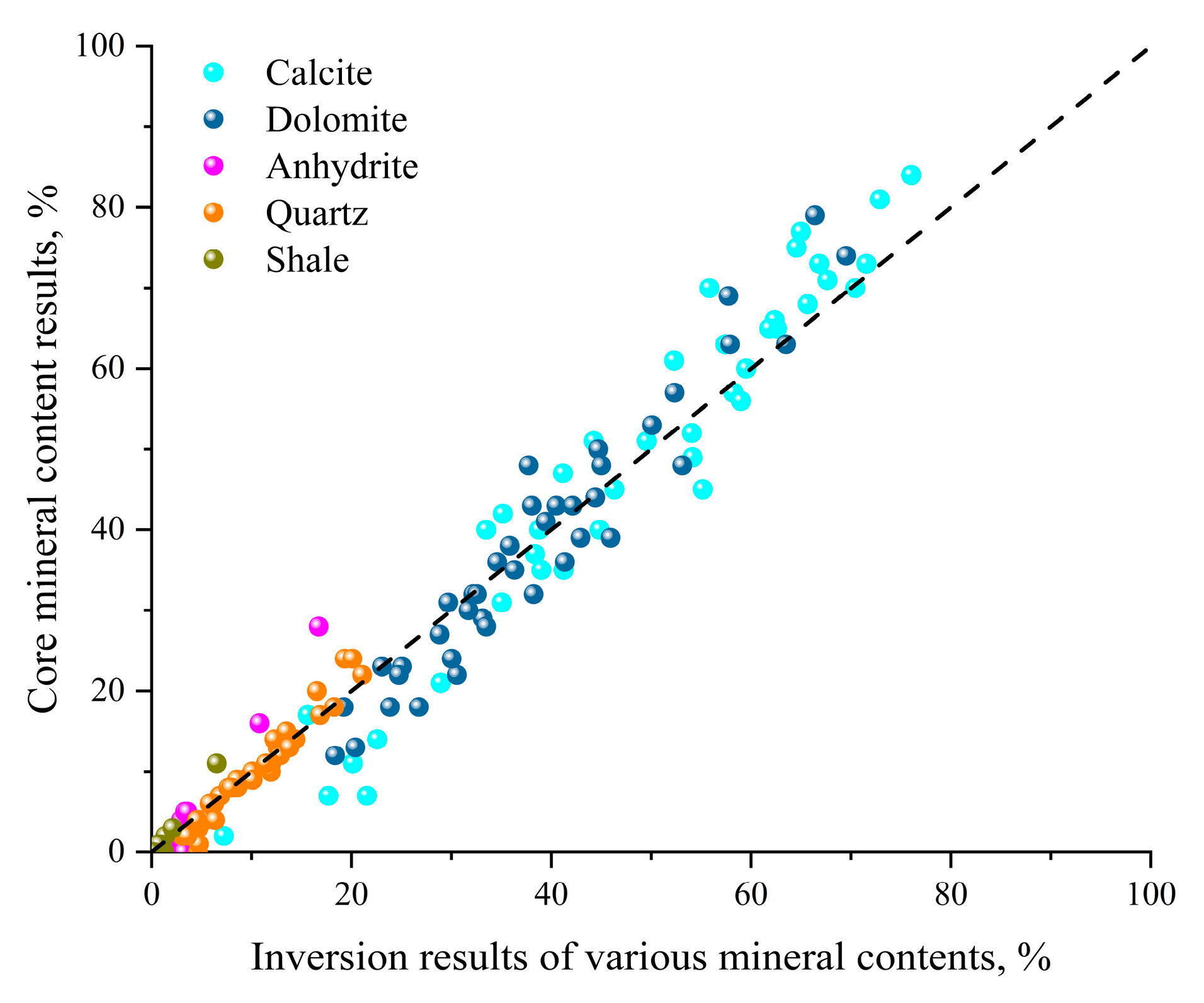
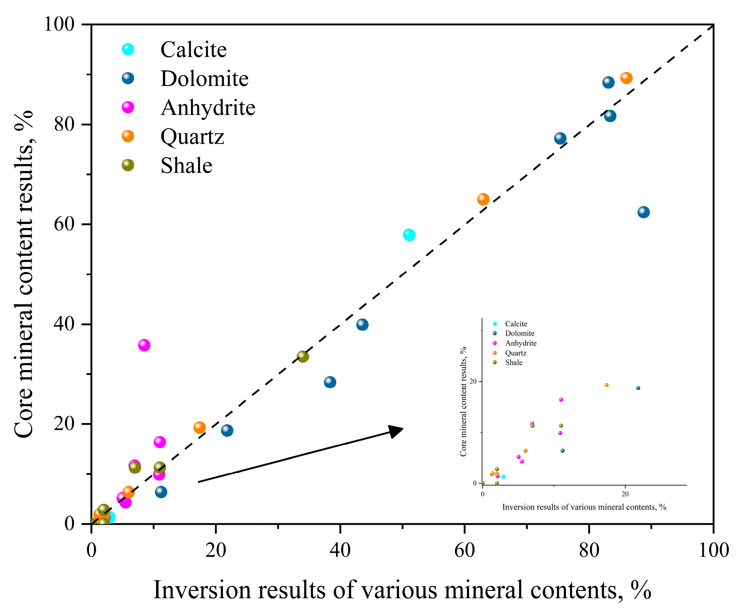
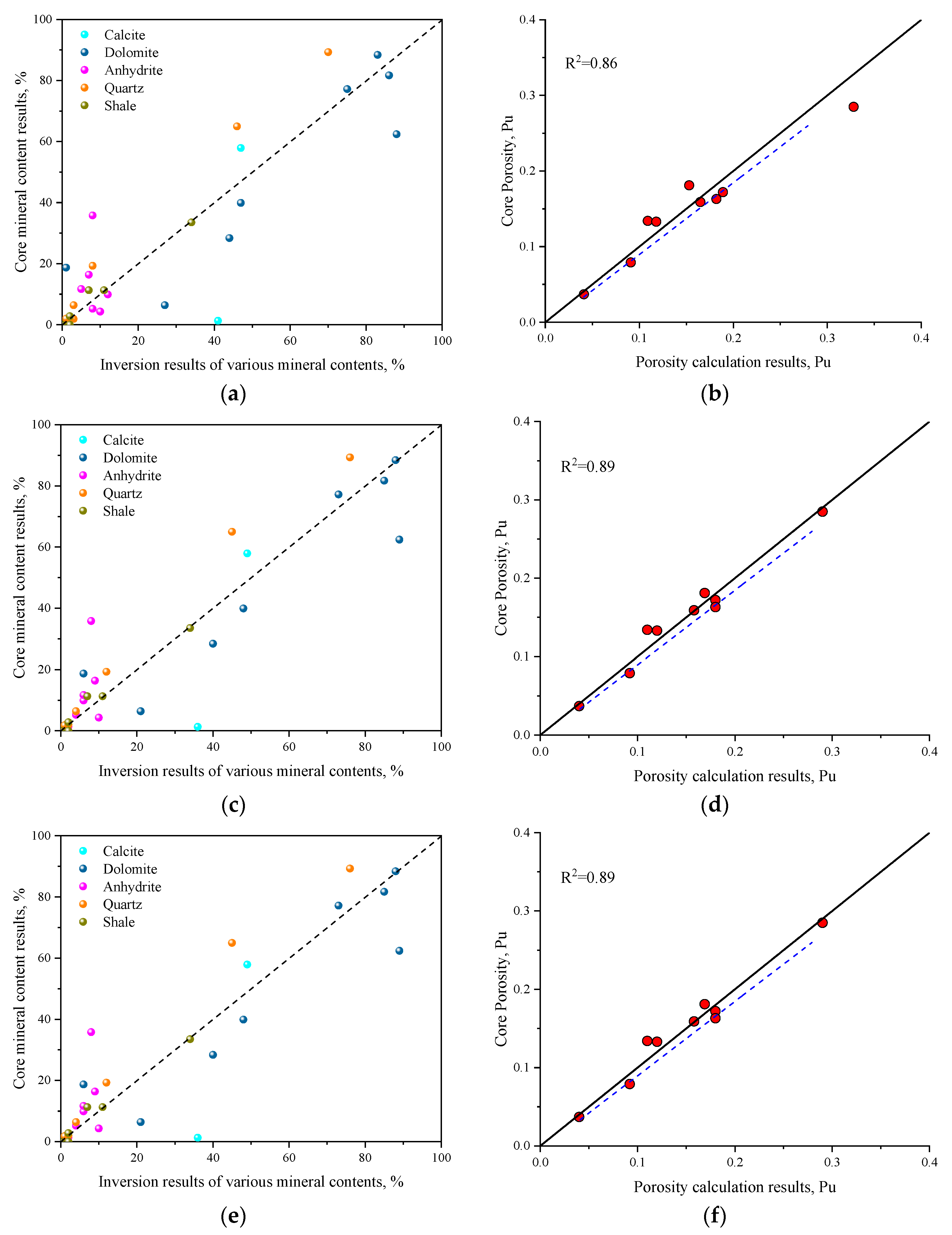
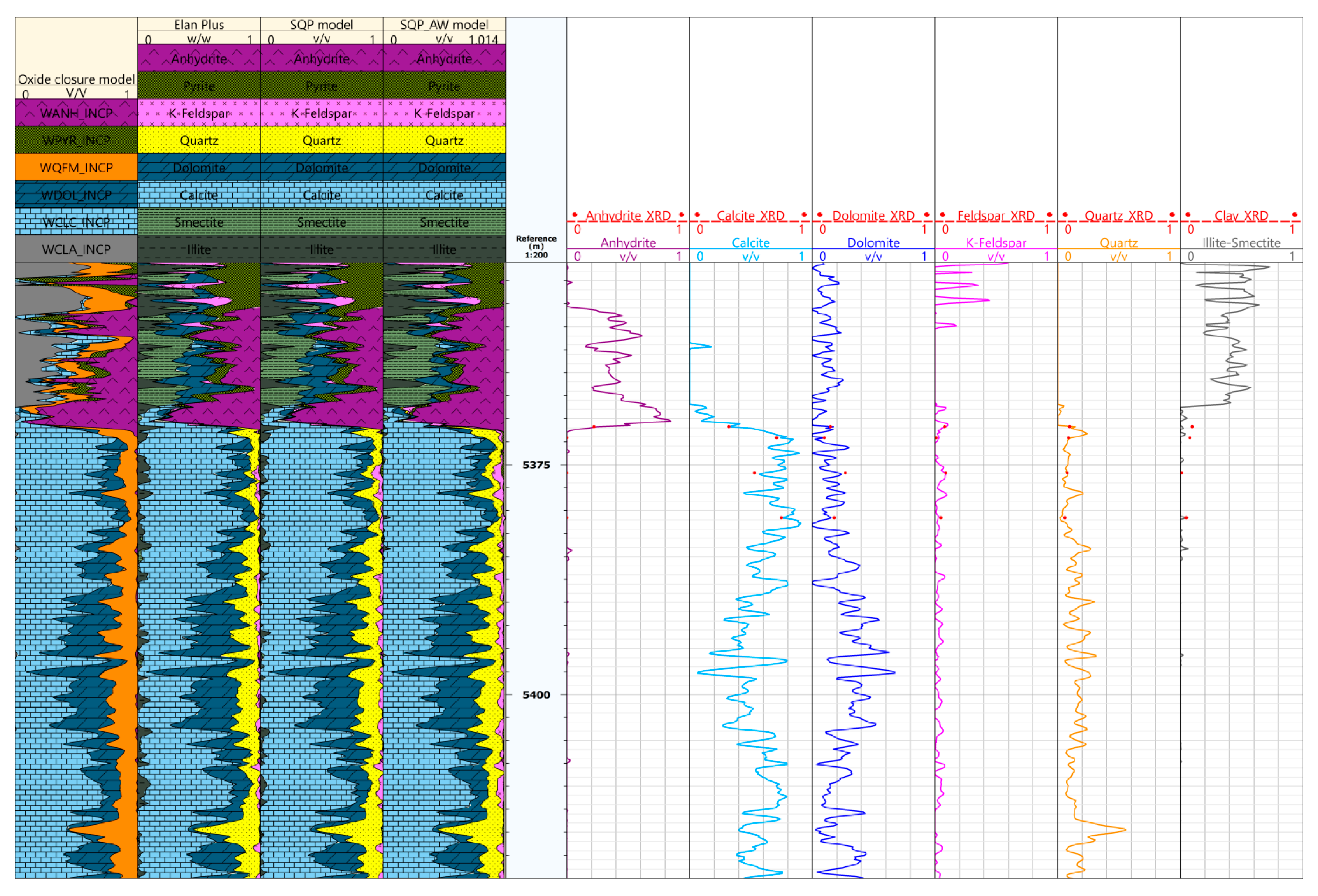
4.2. Mineral Content Inversion Results

Based on the coefficients of the system of equations and the respective equation weights, mineral contents were inverted. Additionally, the 40 sets of core experimental data used for coefficient calibration were subjected to cross-validation. The resulting comparison between the computed data and core data is presented in the intersection diagram shown in Figure 5. The results indicate strong agreement between the calculated and core data, with an overall goodness of fit (R²) of 0.91.

For the core samples described above, the calculation errors in the content of each mineral are presented in the error table (

Table 3. Calculation error table of contents of various minerals.

Evaluating Index	Quartz	Calcite	Dolomite	Anhydrite	Shale
Mean Relative Error (%)	5.5	9.4	10.2	24.6	11.7
Mean Absolute Error (%)	3.2	4.9	5.2	5.9	1.8
R2 (Pu)	0.92	0.84	0.82	0.61	0.73

). Table 3 displays the average absolute error, average relative error, and R² for the calculated mineral contents compared with the core data. The data indicate that the prediction accuracy for quartz, dolomite, and calcite contents is high, while the prediction accuracy for anhydrite is the lowest. An analysis of the intersection diagram (Figure 5) shows that the anhydrite content is relatively low, with its concentration in the 40 core samples being below 30%, and most samples have less than 10% anhydrite. As a result, despite an average absolute error of 5.9% for anhydrite, the highest average relative error was observed. Similarly, for shale content, since this mineral can be calculated by using the natural gamma curve, the solution from the system of equations is not necessary in multi-mineral inversion.

The results of the evaluation above demonstrate the effectiveness of the model. To further validate the accuracy and generalizability of the method here proposed, an application and verification were conducted by using data from Well A, located in the Santos Basin, which was not included in model construction. The application was performed on the Asmari Formation of Well A. Figure 6 presents the application results, which are displayed across fourteen panels: first, the depth panel, showing the measurement depth of the curves; second, the stratigraphy panel, which includes the specific stratigraphy of the Asmari Formation; third, the lithology curve panel, which includes natural potential curves, borehole diameter curves, drill bit diameter, and natural gamma logging curves; fourth, the porosity logging curve panel, which contains the sonic travel-time logging curve, the compensated density logging curve, and the compensated neutron logging curve; fifth, the resistivity panel, showing three resistivity curves with different detection radii; sixth, the modulus curve panel, which includes the shear modulus and bulk modulus curves calculated from the sonic travel-time curve, the shear wave travel-time curve, and the compensated density curve; seventh, the nuclear magnetic resonance logging curve panel; eighth, the mineral profile panel, obtained by overlaying the mineral content calculation results, with unfilled segments corresponding to porosity values; panels nine to thirteen display the calculated contents of anhydrite, calcite, dolomite, quartz, and shale, respectively, along with the corresponding XRD analysis results from core samples (the XRD results were converted by using core porosity and not pure mineral proportions to ensure comparability); the fourteenth panel shows the porosity panel, which includes both the porosity calculation curve and core porosity, where porosity was calculated by applying a volume model after obtaining the weighted rock density from mineral content calculations.

The analysis of Figure 6 reveals that section MB1 is primarily composed of gypsum, while sections A1 to A3 predominantly present dolomite with minor interbedded mudstone layers. The lithology in section B is more complex, with an increase in mudstone layers and the development of dolomite, calcite, and quartz. A comparison of the calculated mineral content with core sample results shows a high degree of consistency, although some discrepancies are noted. The XRD results indicate that at a depth of 3032 m, the sample contains 100% gypsum. Figure 7 presents the corresponding Scanning Electron Microscopy (SEM) image, which shows pure gypsum. Despite this, the log responses, including the compensated density, sonic travel time, and compensated neutron logs, do not exhibit significant variations. The compensated density log, for instance, shows only a slight increase. This limited fluctuation may be due to the vertical resolution constraints of the logging curves, which prevent the effective identification of such unusual samples. Apart from these special cases, the comparison of mineral content calculations with core experiment results for the remaining eight sample sets, shown in Figure 8, demonstrates that the calculated and core results are evenly distributed on both sides of the zero-error line, with a goodness of fit of 0.87.

5. Discussion

5.1. Advantages of the New Method

Traditional methods rely solely on conventional logging curves for mineral content inversion; in this study, we extend the inversion equation by incorporating modulus parameters and nuclear magnetic porosity. The feasibility of using the shear and bulk moduli has been demonstrated by previous researchers, particularly for distinguishing dolomite and calcite in carbonate rocks. Li et al. [36] introduced the nuclear magnetic porosity equation for extension and calibrated the coefficients in the equation by using micro-image stitching scans, achieving successful results in tight sandstones. Unlike previous authors, we verify these methods by combining thin-section data, as shown in Figure 9, with Figure 9a showing the actual core thin-section data and Figure 9b presenting a correlation plot between the pore face percentage and core porosity extracted from the thin-section data for the study area. The results indicate a weak correlation between the two. Figure 9c provides further clarification to address this issue: the image data from cross-sections, such as those from core thin sections, only represent individual planes and fail to fully capture the three-dimensional characteristics of the core. Additionally, the pore face shape is complex. Under ideal conditions, as shown in Figure 9d, there is a conversion relationship between porosity and pore face percentage for regular cubic and spherical geometries. However, in actual formations, the reservoir’s strong heterogeneity makes the real situation more complex than the theoretical case; therefore, using image data for coefficient calibration introduces certain risks.

We utilize the SQP_AW model for coefficient calibration, mitigating the risks of using two-dimensional data to represent three-dimensional characteristics. The results from the practical application show good agreement with core data.

We conducted a comparative analysis across three groups to further validate the effectiveness and innovation of the proposed method. The first group employed the proposed method in combination with conventional logging curves to invert mineral content, gradually adding additional curves. The second group used conventional logging curves along with two modulus curves for inversion. The third group incorporated conventional logging curves, two modulus curves, and nuclear magnetic porosity curves to invert the mineral content. In all cases, eight samples from Well A were used for comparison, and the results are shown in Figure 10.

Figure 10a represents the inversion results for the first group, while Figure 10b displays the correlation plot between the porosity derived from the inversion results and the core porosity, based on a volume model. The goodness of fit reaches 0.86, indicating that the proposed method combined with conventional logging curves can effectively invert the mineral content. While some samples exhibited discrepancies, the main minerals could be accurately quantified, and the corresponding porosity effectively reflected the actual core porosity. As additional curves were introduced, the precision of dolomite and calcite improved with the inclusion of two modulus curves, resulting in a goodness of fit for porosity calculations of 0.89. When all curves were used, the prediction accuracy for quartz improved further, and the goodness of fit for porosity reached its highest value, 0.91.

The average relative errors in mineral content inversion and porosity across the three groups were statistically analyzed. The average relative error in each group’s mineral content was weighted based on the actual core composition, which yielded errors of 9.45%, 7.21%, and 6.59% for the first, second, and third groups, respectively. The corresponding average relative errors in porosity were 8.1%, 7.6%, and 7.1%, respectively. These results demonstrate that the proposed method, when combined with conventional logging curves, can effectively invert mineral content and compute porosity. The inclusion of modulus curves enhances the prediction accuracy for dolomite and calcite, while the introduction of nuclear magnetic porosity curves improves the evaluation of quartz content. Overall, the addition of curves leads to better accuracy in mineral content evaluation and porosity prediction.

5.2. Extensibility of the New Method

The method proposed in this study demonstrated good performance when applied to wells with conventional logging data, array data, and nuclear magnetic resonance (NMR) data. Additionally, the method was evaluated for wells for which elemental logging data had been collected.

A trial calculation was conducted for Well B in the Brazilian block of the Santos Basin, which collected elemental logging data. The analysis focused on the formation interval from 5353 m to 5773 m in depth. XRD data and a core thin-section analysis revealed that the primary minerals in this interval were calcite and dolomite, with minor amounts of quartz and potassium feldspar. In the upper section of the formation, small amounts of anhydrite were also observed, while clay minerals, predominantly illite and montmorillonite, were present in low quantities [31].

The relative elemental yields were calculated by using spectral decomposition techniques based on the elemental logging data from the formation. The oxide closure model was then applied to obtain preliminary estimates of the contents of anhydrite, calcite, dolomite, pyrite, the quartz–feldspar–mica (Q-F-M) group, and clay minerals. The preliminary mineral content calculation results are shown in Figure 11, Track 1. However, due to the limitations of the oxide closure model, the computed results were relatively coarse and did not meet the precision required for accurate inversion. The method proposed in this study, specifically the multi-mineral inversion approach based on SQP_AW, which optimizes the inversion equation weights automatically by incorporating XRD data, was applied to enhance the inversion accuracy. Nine elements were selected for inversion, namely aluminum, calcium, iron, potassium, magnesium, sodium, silicon, sulfur, and titanium, with uncertainties of 0.0378, 0.011, 0.018, 0.0026, 0.021, 0.02, 0.016, 0.515, and 0.002, respectively. The inversion minerals chosen were anhydrite, calcite, dolomite, K-feldspar, quartz, illite, smectite, and pyrite.

We compare the SQP_AW model with the SQP model using default parameters and the Elan Plus module from Schlumberger to visually demonstrate the inversion performance of the proposed method. The results show that the inversion outcomes of both the Elan Plus and SQP models closely follow the trend of the oxide closure model (Figure 11, Track 1), as seen in Figure 11, Track 2 and Track 3. However, the inversion results of the Elan Plus and SQP models are more refined, and the distribution of mineral contents more closely aligns with the actual data, indicating that the SQP method can achieve a level comparable to advanced commercial software.

However, the inversion results from the SQP model with default parameters still exhibit certain discrepancies when compared with the XRD data, primarily due to the subjective setting of the weight factors and their associated uncertainties. We further employ the SQP_AW model to automatically optimize the weight factors to address this issue. The optimized mineral composition is shown in Figure 11, Track 4, while Tracks 6 to 11 provide a comparison between the primary mineral contents and the XRD data.

Table 4. Table of optimal weights and average errors for inversion elements.

Element	Optimal Weighting	Average Error (%)
Al	1.85	0.80
Ca	1.73	0.24
Fe	1.95	0.20
K	1.19	0.01
Mg	2.21	0.12
Na	0.69	0.01
Si	1.29	0.09
S	0.88	0.12
Ti	0.65	1.59

summarizes the optimal weights for each inverted element curve in the SQP_AW model under these geological conditions, along with the resulting average errors, which highlight the applicability of the proposed method.

The proposed method is also applicable to elemental logging data. The optimal weights for each element in the study area were determined by integrating actual core sample data, and the inversion accuracy was found to align with the results from the ELAN PLUS module. This demonstrates the reliability of the computed results.

5.3. Limitations of the New Method and Future Research Directions

The novel approach proposed in this study effectively integrates conventional and specialized logging data for mineral content inversion, yielding promising results. Additionally, it proves to be applicable to elemental logging data. The limitations of the method’s application are also addressed and discussed in further detail.

In the absence of elemental logging data, the method proposed in this study facilitates multi-mineral content inversion based on the combination of conventional logging curves with those extracted and calculated from specialized logging data. However, in practical development wells with limited logging series, such as when only a single porosity curve is available, this method may not be effective for mineral content inversion. Similarly, when no array sonic logging data are collected, the shear wave time difference curve cannot be directly extracted, preventing the calculation of the modulus curves required for mineral content estimation, which may lead to reduced inversion accuracy. With the introduction of data-driven approaches, some researchers have used artificial intelligence techniques to invert shear wave time difference curves with promising results [32]. However, the limitation lies in the persistent errors in the inverted shear wave time difference curves, which affect the computed modulus and, consequently, the accuracy of mineral content inversion. The impact of these errors on inversion precision has not yet been effectively assessed. Similarly, in wells lacking nuclear magnetic resonance data, the absence of nuclear porosity leads to a reduction in the number of equations, limiting the types of minerals that can be inverted. This study focuses on carbonate reservoirs; other types of reservoirs, such as igneous rocks and dense sandstones, for which limited data are available [8,9], were not studied. As a future research direction, the method here presented could be applied to other unconventional reservoirs based on the trial calculation, which would allow different improvements to be made.

Furthermore, the existing results, such as the optimal weights of the system of equations, whether for conventional, specialized, or elemental data, were computed specifically for research areas in the Middle East. The feasibility of the weight values derived in this study for areas with different geological backgrounds requires further investigation. Based on the results of this study, it is suggested to recalibrate the weight parameters by integrating the methodology with actual core experimental data from the specific working area, followed by the prediction of multi-mineral contents.

6. Conclusions

We present the SQP_AW model, which combines conventional logging curves and specialized data with the Adam optimization algorithm, for the accurate calculation of reservoir mineral content. Applied to the Asmari Formation of the M oilfield in the Middle East, the model shows promising results for lithology mineral content inversion.

The SQP_AW model effectively inverts mineral content by constructing a linear equation system and optimizing it with the SQP method and the Adam algorithm. The coefficients are calibrated by using core XRD data, and the curve weights are computed under unified uncertainty conditions. For 40 core samples, the model achieved a 0.91 fit with XRD data. When applied to eight additional samples from Well A, the fit reached 0.87, confirming the model’s validity and generalizability.

The new method offers significant advantages over traditional approaches. As it incorporates modulus parameters and expands the nuclear magnetic porosity inversion equation, it improves accuracy in mineral content evaluation (e.g., dolomite, calcite, and quartz) and avoids the risk of using two-dimensional data. Comparative experiments show that adding more curves enhances mineral content and porosity prediction accuracy. The introduction of the elastic modulus and nuclear magnetic porosity allows the average relative error in mineral content to decrease from 9.45% to 6.59% and that in porosity estimation to decrease from 8.1% to 7.1%.

The method is also applicable to wells with elemental logging data and exhibits inversion accuracy comparable to that of advanced commercial software. However, limitations include the impact of missing logging curves (e.g., porosity or sonic data) on inversion accuracy and the regional applicability of the weight values, which require further validation for different geological settings.

References

1. Feng, Z.; Li, X.; Wu, H.; Xia, S.; Liu, Y. Multimineral optimization processing method based on elemental capture spectroscopy logging. Appl. Geophys. 2014, 11, 41–49. [Google Scholar] [CrossRef]
2. Guo, J.; Zhang, Z.; Zhang, C.; Zhao, Q.; Tang, X. Enhanced water saturation evaluation method using an improved electrical efficiency model: A case study of the Mishrif Formation, Iraq. J. Appl. Geophys. 2025, 236, 105656. [Google Scholar] [CrossRef]
3. Tang, X.; Zhou, W.; Yang, W.; Zhang, C.; Zhang, C. An improved method in petrophysical rock typing based on mercury-injection capillary pressure data. Energy Source Part A 2024, 46, 12647–12662. [Google Scholar] [CrossRef]
4. Hollis, C.; Vahrenkamp, V.; Tull, S.; Mookerjee, A.; Taberner, C.; Huang, Y. Pore system characterisation in heterogeneous carbonates: An alternative approach to widely-used rock-typing methodologies. Mar. Petrol. Geol. 2010, 27, 772–793. [Google Scholar] [CrossRef]
5. Hussein, H.S.; Mansurbeg, H.; Bábek, O. A new approach to predict carbonate lithology from well logs: A case study of the Kometan formation in northern Iraq. Heliyon 2024, 10, e25262. [Google Scholar] [CrossRef]
6. Leisi, A.; Shad Manaman, N. Seismic and geomechanical characterization of Asmari formation using well logs and simultaneous inversion in an Iranian oil field. Sci. Rep. 2025, 15, 11276. [Google Scholar] [CrossRef]
7. Stadtműller, M.; Jarzyna, J.A. Estimation of petrophysical parameters of carbonates based on well logs and laboratory measurements, a review. Energies 2023, 16, 4215. [Google Scholar] [CrossRef]
8. Lai, J.; Fan, X.; Liu, B.; Pang, X.; Zhu, S.; Xie, W.; Wang, G. Qualitative and quantitative prediction of diagenetic facies via well logs. Mar. Petrol. Geol. 2020, 120, 104486. [Google Scholar] [CrossRef]
9. Gavidia, J.C.R.; Chinelatto, G.F.; Basso, M.; Souza, J.P.; Soltanmohammadi, R.; Vidal, A.C.; Goldstein, R.H.; Mohammadizadeh, S.M. Utilizing integrated artificial intelligence for characterizing mineralogy and facies in a pre-salt carbonate reservoir, Santos Basin, Brazil, using cores, wireline logs, and multi-mineral petrophysical evaluation. Geoenergy Sci. Eng. 2023, 231, 212303. [Google Scholar] [CrossRef]
10. Lee, H.; Lee, H.P. Formation lithology predictions based on measurement while drilling (MWD) using gradient boosting algorithms. Geoenergy Sci. Eng. 2023, 227, 211917. [Google Scholar] [CrossRef]
11. Zhao, J.; Xu, S.; Peng, H.; Ji, C. Improving Interpretation Accuracy of ECS Mineral Content with Core Analysis Data. Logging Technol. 2018, 42, 49–53. [Google Scholar]
12. Li, D.; Li, X.; Liu, L.; He, W.; Li, Y.; Li, S.; Shi, H.; Fan, G. Prediction on rock strength by mineral composition from machine learning of ECS logs. Energy Geosci. 2025, 6, 100386. [Google Scholar] [CrossRef]
13. Sun, J.; Jiang, D.; Yin, L. A method for determining mineral content by formation element logging. Nat. Gas Ind. 2014, 34, 42–47. [Google Scholar]
14. Zhao, J.; Chen, H.; Yin, L.; Li, N. Mineral inversion for element capture spectroscopy logging based on optimization theory. J. Geophys. Eng. 2017, 14, 1430–1436. [Google Scholar] [CrossRef]
15. Mohamed, A.; Ibrahim, E.; Sabry, A. Petrophysical characteristics of Wakar formation, Port Fouad marine field, north Nile delta, Egypt. Arab. J. Geosci. 2013, 6, 1485–1497. [Google Scholar] [CrossRef]
16. Parra, J.; Emery, X. Geostatistics applied to cross-well reflection seismic for imaging carbonate aquifers. J. Appl. Geophys. 2013, 92, 68–75. [Google Scholar] [CrossRef]
17. Gao, C. An Optimum Algorithm to Inverse Geochemical Logging Data to the Composition of Rock Materials. J. Petrol. Nat. Gas 1999, 21, 26–28. [Google Scholar]
18. Amosu, A.; Sun, Y. MinInversion: A program for petrophysical composition analysis of geophysical well log data. Geosciences 2018, 8, 65. [Google Scholar] [CrossRef]
19. Li, J.; Lu, S.; Wang, M.; Chen, G.; Tian, W.; Jiao, C. A novel approach to the quantitative evaluation of the mineral composition, porosity, and kerogen content of shale using conventional logs: A case study of the Damintun Sag in the Bohai Bay Basin, China. Interpretation 2019, 7, 83–95. [Google Scholar] [CrossRef]
20. Pan, B.; Xue, L.; Huang, B.; Yan, G.; Zhang, L. Evaluation of volcanic reservoirs with the “QAPM mineral model” using a genetic algorithm. Appl. Geophys. 2008, 5, 1–8. [Google Scholar] [CrossRef]
21. Boiger, R.; Churakov, S.V.; Ballester Llagaria, I.; Kosakowski, G.; Wüst, R.; Prasianakis, N.I. Direct mineral content prediction from drill core images via transfer learning. Swiss J. Geosci. 2024, 117, 8. [Google Scholar] [CrossRef]
22. Zhang, H.; Wu, W.; Song, X. Well Logs Reconstruction Based on Deep Learning Technology. IEEE Geosci. Remote Sens. 2024, 21, 7501205. [Google Scholar] [CrossRef]
23. Wang, J.; Cao, J.; You, J. Reconstruction of logging traces based on GRU neural network. Oil Geophys. Prospect. 2020, 55, 510–520. [Google Scholar] [CrossRef]
24. Tariq, Z.; Gudala, M.; Yan, B.; Sun, S.; Mahmoud, M. A fast method to infer Nuclear Magnetic Resonance based effective porosity in carbonate rocks using machine learning techniques. Geoenergy Sci. Eng. 2023, 222, 211333. [Google Scholar] [CrossRef]
25. Wang, Y.; Mao, Z.; Hu, C.; Li, G.; He, W.; Ma, F. Research on evaluation method of rock mineral composition content by logging based on deep convolutional neural networks. Prog. Geophys. 2023, 38, 748–758. [Google Scholar]
26. Wang, J.; Cao, J.; You, J.; Cheng, M.; Zhou, P. A method for well log data generation based on a spatio-temporal neural network. J. Geophys. Eng. 2021, 18, 700–711. [Google Scholar] [CrossRef]
27. Zhai, X.; Gao, G.; Li, Y.; Chen, D.; Gui, Z.; Wang, Z. Reconstruction method of logging curves by 2D convolutional neural network integrating attention mechanism. Oil Geophys. Prospect. 2023, 58, 1031–1041. [Google Scholar]
28. Guo, J.; Zhang, Z.; Xiao, H.; Zhang, C.; Zhu, L.; Wang, C. Quantitative interpretation of coal industrial components using a gray system and geophysical logging data: A case study from the Qinshui Basin, China. Front. Earth Sci. 2023, 10, 1031218. [Google Scholar] [CrossRef]
29. Moradi, M.; Kadkhodaie, A.; Taheri, M.R.; Chenani, A. Estimation of porosity distribution from formation image logs and comparing the results with NMR log analysis: Implications for the heterogeneity analysis of carbonate reservoirs with an example from the Asmari reservoir, southwest Iran. J. Afr. Earth Sci. 2024, 218, 105366. [Google Scholar] [CrossRef]
30. Taheri, K.; Alizadeh, H.; Askari, R.; Kadkhodaie, A.; Hosseini, S. Quantifying fracture density within the Asmari reservoir: An integrated analysis of borehole images, cores, and mud loss data to assess fracture-induced effects on oil production in the Southwestern Iranian Region. Carbonates Evaporites 2024, 39, 8. [Google Scholar] [CrossRef]
31. Lv, H.; Guo, J.; Gu, B.; Liu, Y.; Wang, L.; Wang, L.; Zhu, Z.; Zhang, Z. High-Precision Permeability Evaluation of Complex Carbonate Reservoirs in Marine Environments: Integration of Gaussian Distribution and Thomeer Model Using NMR Logging Data. J. Mar. Sci. Eng. 2024, 12, 2135. [Google Scholar] [CrossRef]
32. Lv, H.; Guo, J.; Gu, B.; Zhu, Z.; Zhang, Z. A fracture identification method using fractal dimension and singular spectrum entropy in array acoustic logging: Insights from the Asmari Formation in the M oilfield, Iraq. J. Appl. Geophys. 2025, 233, 105631. [Google Scholar] [CrossRef]
33. Khazaie, E.; Noorian, Y.; Moussavi-Harami, R.; Mahboubi, A.; Kadkhodaie, A.; Omidpour, A. Electrofacies modeling as a powerful tool for evaluation of heterogeneities in carbonate reservoirs: A case from the Oligo-Miocene Asmari Formation (Dezful Embayment, southwest of Iran). J. Afr. Earth Sci. 2022, 195, 104676. [Google Scholar] [CrossRef]
34. Ge, Y.; Wu, W.; Yang, C.; He, L.; Hu, G. Calculation of elemental logging yield and analysis of influencing factors. Prog. Geophys. 2020, 35, 950–954. [Google Scholar] [CrossRef]
35. Kumar, V.; Sondergeld, C.; Rai, C.S. Effect of mineralogy and organic matter on mechanical properties of shale. Interpretation 2015, 3, 9–15. [Google Scholar] [CrossRef]
36. Li, C.; Hu, F.; Yuan, C.; Li, X.; Li, C.; Liu, X. Determining multi-mineral compositions in tight reservoirs using a combination of NMR and conventional logging methods. J. Petrol. 2018, 39, 1019–1027. [Google Scholar] [CrossRef]
37. Quirein, J. A coherent framework for developing and applying multiple formation models. In Proceedings of the Society of Professional Well Log Analysts 27th Annual Logging Symposium, Houston, TX, USA, 9–13 June 1986; pp. 1–17. [Google Scholar]
38. Kingma, D.P.; Ba, J. Adam: A method for stochastic optimization. arXiv 2014, arXiv:1412.6980. [Google Scholar] [CrossRef]
39. Yi, D.; Ahn, J.; Ji, S. An effective optimization method for machine learning based on ADAM. Appl. Sci. 2020, 10, 1073. [Google Scholar] [CrossRef]
Figure 1. Core photos of Asmari Formation in M oilfield.
Processes 13 01954 g001
Figure 2. Experimental results of core XRD of Asmari Formation in M oilfield (taking sample 38 as an example).
Processes 13 01954 g002
Figure 3. Core mineral content distribution pie chart of Asmari Formation in M oilfield.
Processes 13 01954 g003
Figure 4. Solution of equation system.
Processes 13 01954 g004
Figure 5. The cross plot of the calculation results of 40 groups of core XRD data and the core results.
Processes 13 01954 g005
Figure 6. Mineral content calculation results of Asmari layer group in Well A1.
Processes 13 01954 g006
Figure 7. Scanning Electron Microscopy image of core sample at 3032 m of Well A1 (anhydrite content: 100%).
Processes 13 01954 g007
Figure 8. The cross plot of mineral content calculation results and core experimental results of 8 groups of samples from Well A1.
Processes 13 01954 g008
Figure 9. The demonstration of coefficient selection in nuclear magnetic porosity equation: (a) the actual core casting thin-section image; (b) the cross plot of the surface porosity and core porosity extracted from casting thin-section data in the study area; (c) a two-dimensional image that characterizes the situation diagram of the three-dimensional pore space; (d) the relationship between porosity and surface porosity in the ideal sphere model.
Processes 13 01954 g009
Figure 10. Comparison of three different mineral content inversion effects for Well A data: (a) the cross plot of mineral content inversion results and core results based on conventional logging curves; (b) the cross plot of porosity and core porosity calculated with the inversion of mineral content using conventional logging curves; (c) the cross plot of mineral content inversion results and core results based on conventional logging curves and two modulus curves; (d) the cross plot of porosity and core porosity calculated with the inversion of mineral content by conventional logging curve and two modulus curves; (e) the cross plot of mineral content inversion results and core results by combining conventional logging curves, modulus curves, and nuclear magnetic porosity; (f) the cross plot of porosity and core porosity calculated with the inversion of mineral content by conventional logging curve, two modulus curves, and nuclear magnetic porosity.
Processes 13 01954 g010
Figure 11. The new method and ECS logging data are applied to the calculation results of mineral content in Well B of the oilfield.
Processes 13 01954 g011