Fatigue Life Prediction of Five MW Wind Turbine Blade Based on Long-Term Wind Speed Simulation

Abstract

This paper studies the load spectrum and fatigue life estimation method of large wind turbine blades. A method based on the wind speed spectrum and stress response at each wind speed is proposed to calculate the response spectrum of the dangerous part of the blade. The response of the blade at each wind speed is obtained by finite element analysis. Considering the limited wind speed data, it is not enough to cover the whole situation of blade life experience, which will bring great discreteness to the blade fatigue life estimation method proposed in this paper. In this paper, the Markov chain Monte Carlo method is used to predict enough wind speed data to reduce the discreteness of life estimation. Because the traditional linear fatigue damage accumulation theory fails to consider the impact of loads below the fatigue limit on fatigue damage, this paper uses a fatigue damage theory based on fuzzy theory, introduces appropriate membership functions, and fully considers the impact of loads below the fatigue limit on fatigue damage. The calculation results are more in line with the actual situation.

1. Introduction

The environmental problems caused by the massive use of fossil energy have increasingly attracted people’s attention. As people’s voices on environmental protection are raised, the utilization of clean and renewable energy sources has become the focus of people’s attention. In order to realize the sustainable development of society and reduce the dependence on fossil energy, solar energy, wind energy, tidal energy, geothermal energy and many other green and clean energies began to ascend to the stage of history and become the mainstream direction of future energy development in the world. In 2024, China’s domestic installed capacity will increase by 14,388 units, with a capacity of 86.99 million kW, an increase of 9.6% year-on-year; in the same year, the total installed capacity was more than 209,000 units, with a total installed capacity of 561.26 million kW [1]. As the main form of wind energy utilization, the wind power generation industry has been widely emphasized in China.

As the core component of the generator set, the stable operation of the generator set is affected to a large extent by the performance of the blade. Its manufacturing cost accounts for 15% to 20% of the wind turbine equipment, and a large part of wind farm accidents is due to the unstable operation of the blade. Ensuring the quality of the blade is an important factor in ensuring the stable operation of the wind turbine and the safety of the wind farm. Wind turbine blades in operation will be subjected to extreme load and fatigue load; the actual situation is greater than the material strength limit of the extreme load and seldom leads to blade failure; the fatigue load amplitude is lower than the strength limit of the material, but due to the significantly higher number of cycles, it is usually the leading cause of fatigue damage to the blade. Research shows that the blade service life depends mainly on the fatigue life; therefore, the prediction of the blade’s fatigue life is of great significance. Based on the fracture mechanics theory, Aghajani et al. proposed a new multiaxial fatigue damage prediction model for wind turbine blades; interfiber characteristics and fatigue reduction of fiber are separately treated and simulated in this research, and the mechanism of composite blade damage generation and accumulation under multiaxial fatigue load conditions are analyzed [2]. According to the fatigue failure criterion, Kou selects blade stiffness as the characteristic quantity of the blade performance and proposes the blade acceleration model (AM). Then, the model of the blade stiffness attenuation path is established by using the Gamma process. Finally, the life of the full-size megawatt blade is predicted to be about 20 years by combining the proposed acceleration model and the blade stiffness degradation model [3]. Based on the measured wind speed and direction data at the hub of the wind turbine, Zhao Qin uses the research ideas of ‘non-Gaussian characteristics analysis of wind‘ and ’fatigue life analysis of blades‘ to systematically study the joint distribution probability model of non-Gaussian wind speed and direction and the life calculation model of blades in the whole wind direction range [4]. After obtaining the fatigue load of each section of the blade under different working wind speeds using GH Bladed software, Han Tongtong carried out a transient analysis with a remote point. Simplifying the section load into a remote point load can significantly improve the calculation efficiency. NCode compiles the stress load spectrum, and the fatigue life is predicted by fuzzy mathematics theory [5]. Zhang Zhewei carried out damage identification and location of small wind turbine blades with damage through experiments and carried out fluid–solid coupling simulation using finite element analysis software. The obtained data were used to study the residual fatigue life of wind turbine blades under four damage conditions [6]. Ma proposed a model to describe the constant life fatigue limit of typical glass fiber-reinforced plastic (GRP) composites. Compared with the classical model, it is pointed out that there are differences in the damage accumulation mode of GRP in the tensile and compressive stages. It is proved that the constant life fatigue limit curve is asymmetric and bell-shaped. The prediction effect of the model in stress–life data is compared and analyzed [7]. Yu takes the 1.5 MW blade as the research object and uses the fatigue load spectrum of the actual 1.5 MW blade during service. Based on the generalized stress–life curve of the blade material, the fatigue damage accumulation model of the blade under random load is used to calculate the total fatigue damage of the blade and predict the fatigue life. The prediction results of blade life are close to the field test results, which proves the correctness of the proposed blade fatigue life evaluation method [8]. According to the condition that the initial static strength of the composite material obeys the two-parameter Weibull distribution, Zhao assumed the relationship between the residual strength decay rate and the residual strength and constructed the initial static strength [9].

In summary, in past research, the key to predicting the fatigue life is to calculate the fatigue damage of the blade, so choosing a suitable method to solve the fatigue damage of the blade is the key to estimating the life of the blade and the premise of calculating the fatigue damage of the blade is to obtain the blade response and then obtain the stress spectrum. Some scholars measured the stress spectrum of the blade by installing a strain gauge at the root of the blade. However, determining the installation position of the strain gauge is a problem. In addition, due to the difficulty in obtaining measured load data for large wind turbines, most scholars primarily obtain relevant load data through analysis and simulation for the fatigue analysis of wind turbine blades. Some scholars calculate the static load of the dangerous part of the blade under each working wind speed using the fluid–solid coupling method and then obtain the stress spectrum by combining the annual distribution of wind speeds. In this paper, a fluid–solid coupling method is proposed to obtain the corresponding instantaneous static response sequence by combining the static load and the dynamic wind speed sequence. The instantaneous static response results are used to calculate the damage generated during the blade working process. Considering that the calculation results of this method will be affected by the randomness of wind speed when the wind speed data is insufficient, in order to make up for this, the wind speed prediction is used to simulate enough reasonable wind speed data to eliminate this effect. The test data in Reference [10] show that the dynamic response of the blade is closely related to the change in wind speed, and the transient response of the blade is not entirely consistent with the instantaneous change in wind speed. 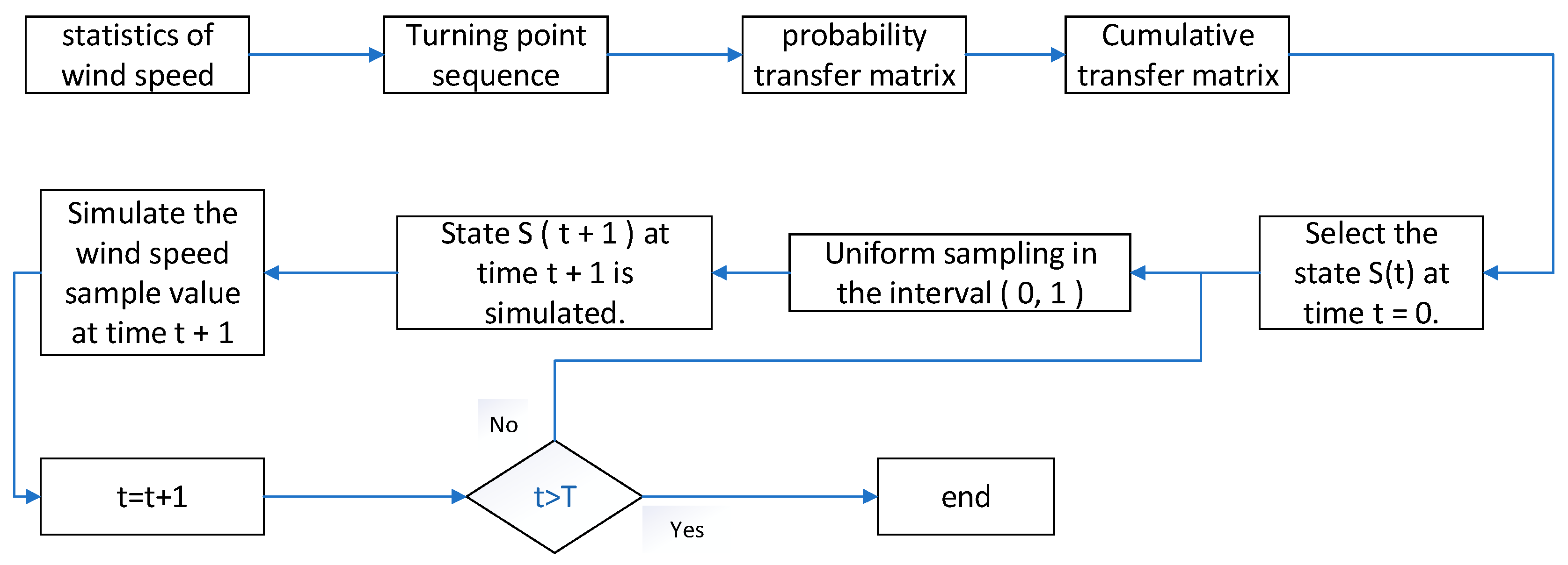If the transient response of the blade is entirely consistent with the change in the corresponding wind speed, that is, the instantaneous dynamic response of the blade with the change of wind speed is approximated to the corresponding instantaneous static response, the vibration of the strain signal is much more severe than the original [11]. From the perspective of fatigue, it can be considered that this assumption will cause more damage to the blade; that is to say, calculating the fatigue life of the blade under this assumption is a more conservative and feasible engineering estimation method. Considering that this method is not enough to cover all cases of blade service life in wind speed data, the estimated fatigue life will also have a lot of discreteness. This paper proposes a fatigue life prediction method considering long-term wind speed simulation to reduce the influence of wind speed randomness on the prediction results. In this paper, the wind speed prediction model is required to predict as much instantaneous wind speed data as possible. When evaluating the reliability of offshore wind power, Chao uses the time series properties of wind speed series to predict the wind speed for a long time by using the MCMC model and ARMA model, respectively. The final results show that the prediction results of the ARMA model contain negative values, while the MCMC model is more in line with the actual situation [12]. Based on statistical methods and neural network methods, Li designed a multi-neural network data fusion algorithm to predict the hourly wind speed in the following year. The results show that the average absolute error is small, and the wind speed trend is close to the actual results [13]. Under comprehensive consideration, this paper uses the MCMC model as the wind speed prediction model. The technical roadmap of this paper is shown in Figure 1:

2. Long-Term Forecasts of Wind Speed

2.1. Markov Chain

A Markov chain is a special type of discrete stochastic process that is used to describe the transfer process between events. The Markov process requires that the future state of things is independent of the past state and depends only on the present state. If the discrete stochastic process $\{X_k,k=0,1,2\dots \}$ is a stochastic process that takes a finite number of states, the states that may be achieved during the process will be represented by the set of positive integers $\{1,2,3\dots \}$. Then, the state transfer probability for any moment has $P\left(X_t=j|X_{t-1}=i\right)=p_{ij}$, which is invariant in time. The moments used to identify and define these conditional probabilities are represented as a time-step equidistant Delta. An m × m transfer probability matrix can then be formulated.

$$p=\left[\begin{array}{cccc}{p}_{11}& p_{12}& \cdots & p_{1n}\\ p_{21}& p_{22}& \cdots & p_{2n}\\ ⋮& ⋮& \ddots & ⋮\\ p_{m1}& p_{m2}& p_{m3}& p_{mn}\end{array}\right]$$

(1)

According to this representation, each row of the matrix corresponds to the current state of the process, and each column points to the possible next state. For example, p56 represents the transition probability that the current state is 5 and the next is 6. The rows of the matrix add up to 1 $({\displaystyle \sum p_{ij}}=1)$ because the cumulative result of each row corresponds to the probability of transition from the current state to any possible state. The estimation of the matrix term is

$$p_{ij}={\displaystyle \frac{n_{ij}}{{\displaystyle \sum _{j=1}^n{n}_{ij}}}}$$

(2)

$n_{ij}$ is the number of transitions from state i to state j.

2.2. Markov Chain Monte Carlo Simulation (MCMC Simulation)

This paper completes the MCMC simulation of wind speed using the Gibbs sampling method. Firstly, the wind speed is divided into states, the state interval is divided by 1 m/s interval, the wind speed state is used to represent the wind speed distribution, and the cumulative probability transfer matrix Pcum is calculated by Equation (2). In the case of a first-order Markov chain, each row i of the cumulative transition matrix corresponds to the discrete cumulative distribution function Fi of the next transformation. Let t = 0, according to the occurrence probability of wind speed state, the initial wind speed state Si is randomly selected when t = 0, and a random number q evenly distributed in an interval $(0,1)$ is randomly selected. If it falls between the elements P_cum(ij) and P_cum(1, j + 1), the next state is considered to be j + 1, and this process is repeated until the sampling length T is satisfied. The elements of the cumulative probability transfer matrix are

$$P_{cum}(ij)=\left\{\begin{array}{cc}0& j=1\\ {\displaystyle \sum _{l=1}^{j-1}{p}_{il}}& 1<j\le m+1\end{array}\right.$$

(3)

After obtaining the predicted wind speed state result, the actual wind speed needs to be obtained by the following formula, taking state j as an example:

$$X=X_{j-1}+r(X_j-X_{j-1})$$

(4)

The flowchart of the above wind speed simulation method is shown in Figure 2.

Figure 3 is the wind speed data recorded in a particular area of Beijing from 2020 to 2022 [14], which is accessed through the Xihe platform. In this paper, the wind speed data from 2020 to 2021 is used as the original data, and the wind speed data for the next year is predicted by the Monte Carlo method. The rationality of wind speed prediction is verified by comparing the statistical characteristics of the data.

According to the method described above, the wind speed results for next year are simulated with the 2020 wind speed series as the original data. The simulation results are shown in Figure 4.

The statistical data shown in

Table 1. Comparison of statistical characteristics of wind speed one year before and after simulation.

Data	Maximum	Minimum	Mean Root	Mean Square	Standard Deviation
Raw data	18.92	0.65	4.60	2.71	5.362813
predicted value	19.58	1	5.16	2.81	5.885126

characteristics that the relative error between the original wind speed and the predicted wind speed is small, which indicates that the MCMC method has a good effect on wind speed simulation.

The wind speed data used to predict the wind speed sequence in this paper is derived from the measured data of a wind farm in the United States for one year. The measurement interval is 10 min. Considering that the working wind speed of the wind turbine is between 3 m/s and 25 m/s, it is necessary to filter out the wind speed other than the working wind speed. The equivalent fatigue stress spectrum required for fatigue analysis can be obtained by combining the long-term wind speed sequence measured by the Markov chain Monte Carlo method with the stress response values at each wind speed obtained below.

3. Numerical Simulation

The operating environment of wind turbines is often very complex, and its overall stress is unpredictable. The blades are deformed and damaged under the interaction of various loads. The deformation and load of the blades under actual operating conditions can be analyzed by the fluid–solid coupling method, which is of great significance for studying the fatigue life of wind turbine blades.

3.1. Three-Dimensional Model of Leaves

The NREL 5 MW wind turbine blade is the research object of this paper. The parameters of the NREL 5 MW wind turbine blade are determined through literature research, and the blade is modeled based on the skin lofting method. Through the coordinate transformation of the cross-section coordinate data of different radial distances of the blade, the coordinate information of each position is saved in DAT format, and the coordinate information is imported into the UG12.0 software using the insertion spline command to generate the airfoil diagram [15]. The blade shape is modeled by the curve group sweeping command, and the web is established at the blade’s 15% and 50% chord lengths. The final result is shown in Figure 5. After completing the modeling work, the blade model is output in IGS format, and the three-dimensional surface of the fan is imported into ANSYS Workbench 2020.

3.2. Fluid Domain Analysis

In this paper, a Multiple Reference Frame (MRF) is used to control the rotation of the blade. In this paper, other wind turbine components, such as the engine room and tower, are not considered. Considering the periodic symmetry of wind turbine blade rotation, in order to save computing resources and improve the calculation speed, as shown in Figure 6, the calculation area only considers one-third of the flow field. The total length of the calculation domain along the free flow direction is 12R, where the inlet to the blade rotation surface is 4R, the radius of the stationary domain is set to 5R, and the length of the rotation domain is set to 5R. The distance between the inlet and the blade rotation surface is 1R, and the radius of the rotation domain is set to 1.5R. According to the incompressible nature of the flow field, the velocity boundary condition at the inlet of the flow field is the Dirichlet condition, the incoming flow velocity is a given velocity, the pressure gradient is 0, the outlet boundary condition is the pressure outlet, that is, the given pressure value, the velocity gradient is 0, and the blade surface adopts the non-slip boundary condition. The K-epsilon wind model is used for the turbulent wind model. The inlet velocity is 11 m/s, 13 m/s, and 19 m/s, respectively. The following is an example of the fluid domain results with a rated wind speed of 11 m/s.

It can be seen from Figure 7 that the high-pressure area on the fan blade is mainly located at the front edge of the pressure, and the pressure gradually decreases from the tip to the blade’s root. The distribution law is obvious. The low-pressure area is concentrated at the tip of the suction surface. The pressure surface is mainly subjected to positive pressure, and the suction surface is mainly subjected to negative pressure. The pressure on the front edge of the blade is higher than the pressure on the trailing edge, and the pressure on the trailing edge of the suction surface is higher than the pressure on the leading edge. The pressure difference on both sides promotes the rotation of the blade. The results are in line with the reality.

3.3. Solid Domain Analysis

The results of the fluid domain calculation are imported into the static calculation module. Similarly, the flow field part needs to be suppressed during the solid domain analysis, and the pressure results of the fluid analysis are loaded onto the blade coupling interface. When the single blade is analyzed in this paper, the blade is regarded as a cantilever beam. Because the blade root is still some distance away from the hub center, it can be considered that the blade root and the rotation center are fixed, and the remote point command is used to impose fixed constraints on the blade root. The thickness of the blade skin is generally 20 mm, and the web’s thickness depends on the blade section’s airfoil chord length [16]. Considering the simplification of the model, the thickness of the blade skin is 20 mm, and the thickness of the web is 30 mm. Considering the long-term operation of the blade in harsh natural environments, the blade should choose materials with high mechanical strength, non-conductivity, corrosion resistance, and light weight, and glass fiber/epoxy material should be selected as the blade skin material. The mechanical properties are shown in

Table 2. Fiberglass/epoxy material properties.

Elastic Modulus/Gpa			Poisson Ratio			Shear Modulus/Gpa
Exy	Eyz	Exz	μxy	µyz	µxz	Gxy	Gyz	Gxz
27.8	28	28	0.21	0.26	0.26	11.1	12.1	12.1

.

The static analysis of the blade under wind speeds of 11 m/s, 13 m/s, and 19 m/s is carried out, and the displacement results of the blade are viewed in the post-processing module. As shown in Figure 8, from the deformation results of the blade, the maximum deformation position of the blade appears at the tip of the blade. The deformation gradually decreases from the tip to the blade’s root, and there is almost no deformation at the blade’s root. With the continuous increase in wind speed, the deformation at the tip of the blade also increases, which is in line with the deformation results of the blade working condition in reality.

The equivalent stress cloud diagram of the blade is shown in Figure 9. From the stress distribution of the blade surface, the maximum stress is located in the transition area from the blade root to the aerodynamic part, which is close to the root of the rib plate and is prone to stress concentration. Therefore, the equivalent stress of the blade is the largest here, and the blade is easily damaged here, which is consistent with the actual situation. And with the increase in wind speed, the equivalent stress of the blade root also increases gradually.

The stress response of the blade at different wind speeds is obtained by numerical simulation. The maximum stress is located at the transition between the aerodynamic part and the blade root part, which can be regarded as a dangerous part, and the maximum stress response at each wind speed is recorded. The results are shown in

Table 3. Stress response at different wind speeds.

Wind Speed (m/s)	Rotor Speed (r/min)	Vibration Response (Mpa)
3	6.9	6.29
5	7.6	11.2
7	8.5	16.2
9	9.6	21.6
11	12.1	32.3
13	12.1	53.3
15	12.1	57.6
17	12.1	68.5
19	12.1	75.5
21	12.1	92.5
23	12.1	101
25	12.1	108

.

The stress spectrum is a prerequisite for estimating fatigue life. In this paper, the corresponding fatigue stress response is obtained by numerical simulation of the blade at various wind speeds. The relationship curve between wind speed and stress value is obtained by curve fitting in the Matlab2016 toolbox. The equivalent fatigue stress spectrum required for fatigue analysis can be obtained by combining the previous wind speed prediction results. The results are shown in Figure 10.

The rain flow counting method was used to count different stress amplitudes and their occurrence frequencies. The results are shown in Figure 11.

4. Material Stress–Life Curve (S–N Curve) and Fatigue Damage Criterion

4.1. S–N Curve of Composite Material

The S–N curve describes the relationship between the stress level and the number of cycles N of the standard part under a specific cyclic symmetrical load loading condition. The general S–N curve obtains the corresponding data through the fatigue test of the standard part, to draw the S–N curve. Another way is to obtain the S-N curve according to the material parameters combined with the empirical formula. Since composite materials have no apparent fatigue limit, the stress when the number of cycles increases to 10⁸ is generally used as its conditional fatigue limit. The exponential function formula is used instead of the measured curve:

$$a{\sigma }_i+\lg N_i=b$$

(5)

In the formula, a and b are material constants, which are dimensionless, $b={\sigma }_b/B$ (b is approximately equal to 10), ${\sigma }_b$ is the static strength of the material; a = 1/B; σ_i represents the stress of the ith level, and N_i represents the maximum number of cycles corresponding to the stress of the ith level.

The above calculation is obtained under symmetrical cyclic stress loading. In reality, the stress ratio of the component under load is generally not −1. Some scholars estimate the fatigue limit through empirical models. In this paper, the conditional fatigue limit under random cyclic characteristics is calculated by the Goodman curve model:

$${\sigma }_a={\sigma }_{-1}\ast (1-{\sigma }_m/{\sigma }_b)$$

(6)

In the formula, ${\sigma }_m$ is the average stress, and ${\sigma }_{-1}$ is the fatigue limit when the stress ratio is −1.

4.2. Fuzzy Miner Linear Fatigue Damage Theory

The fatigue damage theory commonly used in current engineering is the Miner theory. This theory holds that the fatigue damage D of the material can be expressed as the ratio of the number of cycles of stress n to the fatigue limit N of the material under this stress: D = n/N. Under the action of stress cycles with different amplitudes, when the fatigue failure of the component occurs, there are

$${\displaystyle \sum _{i=1}^k\frac{n_i}{N_i}}=1$$

(7)

The linear Miner theory holds that damage cannot be generated when the stress amplitude is lower than the fatigue limit. However, the stress of the material under random load is lower than the fatigue limit, which means there is an intermediate transition fuzzy state where the stress can cause damage to the component. In view of fatigue damage’s fuzziness, some scholars have proposed the discrete Miner fatigue damage accumulation rule of fuzzy theory (hereinafter referred to as the “fuzzy Miner method”).

Many experiments have shown no obvious fatigue limit for composite materials such as fiber glass-reinforced plastics and synthetic resin. For the crack propagation stage, the stress below the fatigue limit will also affect the fatigue damage to a certain extent [17]. A fatigue damage threshold lower than the fatigue limit is defined. When the stress amplitude is lower than the threshold, it is considered that no damage will occur, the fuzzy damage degree is 0, and the stress amplitude in this interval does not affect the fatigue life. When the stress is between the fatigue limit and the fatigue damage threshold, it is considered that damage may occur, and the membership function determines the degree of fatigue damage. When the stress amplitude is greater than the fatigue limit, it is considered that there will be damage, and the fuzzy damage degree is 1.

The membership function is the key to describing the uncertainty of the research object. Only from the membership function can the ambiguity of the research object be described. The fatigue damage caused by random load on the blade is cumulatively increased. Generally, the large membership function is used for analysis and calculation, and the normal distribution membership function is used to describe the ambiguity of the damage caused by wind load on the wind turbine blade.

$$\mu (x)=\left\{\begin{array}{cc}0& x\le a\\ 1-e^{-{({\displaystyle \frac{x-a}{b}})}^2}& x>a,b>0\end{array}\right.$$

(8)

According to the fuzzy uncertainty of the damage of a large number of fatigue test materials under different stresses, it is most reasonable to take the fatigue damage threshold ${\sigma }_0=0.85{\sigma }_{-1}$ as the boundary of the fuzzy characteristics of the material. Through the fitting observation of multiple sets of data, it can be seen that the value of b in the formula is inversely proportional to the stress level, and the value range is (0.05–0.4) ${\sigma }_{-1}$. If the stress above the fatigue limit in the load history of the component has j levels, the fatigue damage of the component under the load history is

$$D={\displaystyle \sum _{i=1}^j\frac{n_i}{N_i}}+{\displaystyle \sum _{i=j+1}^n\frac{n_i}{N_0}\mu ({\sigma }_i)}$$

(9)

In the formula, $N_0$ is the base number of stress cycles. In this paper, $N_0=2\ast {10}^8$.

5. Fatigue Life Calculation

Blade Fatigue Life Calculation

According to the empirical formula mentioned above, the number of cycles under different stress levels and the conditional fatigue limit modified by the Goodman model are calculated. The result is 40.41 Mpa. According to the fuzzy uncertainty of material damage under different stresses in a large number of fatigue tests, it is the most reasonable to set the fatigue damage threshold at $0.85{\sigma }_{-1}$, which is used as the boundary of the material’s fuzzy characteristics. The cumulative duration of wind speed at all levels is calculated by the Webull function. The calculation results are shown in

Table 4. Blade fatigue load spectrum.

Stress Interval (Mpa)	Frequency of Occurrence (Ni)	Maximum Stress	Percentage of Stress Cycle (Ni)
0–5	1558	5	Does not cause fatigue damage
5–10	20,650	10
10–15	42,777	15
15–20	30,778	20
20–25	15,482	25
25–30	17,788	30
30–34	13,655	34
34–40	4418	40
40–45	6732	45	1.32 × 108
45–50	6459	50	1.00 × 108
50–55	6730	55	5.97 × 107
55–60	2715	60	4.44 × 107
60–65	726	65	2.82 × 107
65–70	812	70	1.40 × 107
70–75	149	75	1.15 × 107
75–80	26	80	7.29 × 106
80–85	9	85	4.14 × 106
85–90	1	90	2.16 × 106
90–95	2	95	1.18 × 106

.

According to the Palmgren–Miner theory, the cumulative fatigue damage should be calculated from 40.41 Mpa, and the fatigue damage within 10 years is

$$D={\displaystyle \sum _{i=1}^k\frac{{\mathrm{n}}_i}{N_{\mathrm{i}}}}={\displaystyle \frac{6732}{1.32\times {10}^8}}+{\displaystyle \frac{6459}{1.00\times {10}^8}}+\cdots +{\displaystyle \frac{2}{1.18\times {10}^6}}=5.7\times {10}^{-4}$$

(10)

Considering that the wind load used in this paper is only counted once in 600 s, and the blade is still affected by the wind load at other times, and the damage caused by the calculated wind load is superimposed [18].

$$D1=600\ast D=0.342$$

(11)

$$Y/1=10/D1=29.22 \mathrm{years}$$

(12)

According to the fuzzy Miner fatigue damage theory, the fatigue damage threshold ${\sigma }_0=0.85{\sigma }_{-1}=34.34$. The fatigue damage calculated by the fuzzy Miner fatigue damage theory is

$$D={\displaystyle \sum _{i=1}^j\frac{{\mathrm{n}}_i}{N_{\mathrm{i}}}}+{\displaystyle \sum _{i=j+1}^n\frac{n_i}{N_0}}\mu ({\sigma }_i)=6.9\times {10}^{-4}$$

(13)

$$Y=23.87 \mathrm{years}$$

(14)

The calculation results meet the requirements of the fan’s design life of 20 years, but the error of the fuzzy Miner theory is much smaller than that of the traditional Miner theory, which greatly improves the estimation accuracy and is closer to the actual situation.

6. Conclusions

Based on past research on the life of wind turbines at home and abroad, this paper proposes a method to calculate the blade load spectrum by combining the blade’s transient response with the wind speed value and uses the fuzzy Miner method to estimate the fatigue life of the 5 MW wind turbine. The main conclusions are as follows:

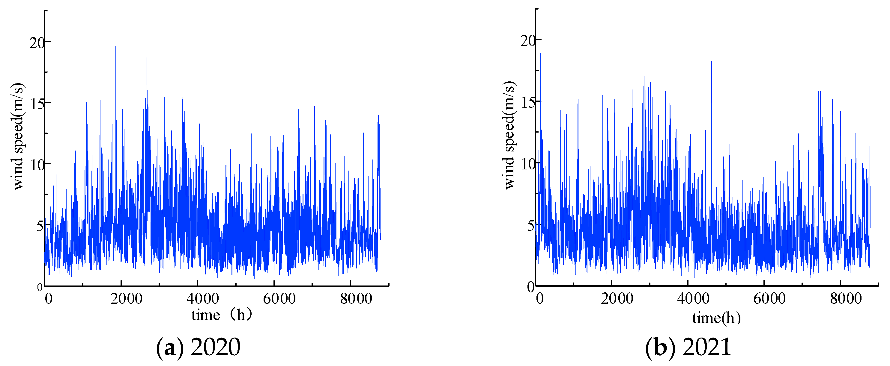
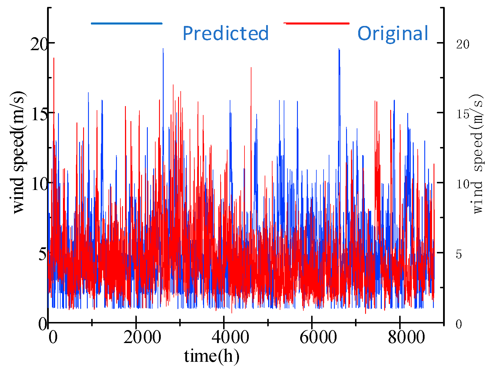
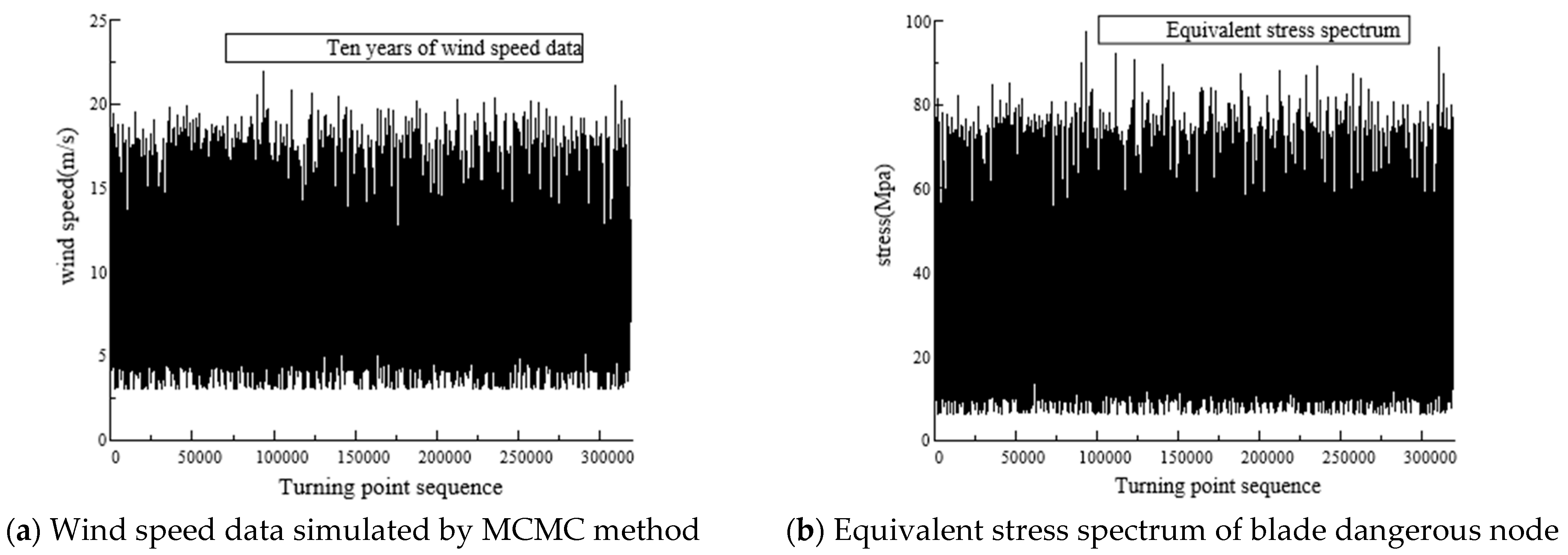
(1) In this paper, the significance of long-term wind speed simulation for fatigue life estimation of wind turbine blades is analyzed. Taking the wind speed data of the Xihe platform for two years as an example, the MCMC method establishes a reliable wind speed prediction model. The prediction results show that the simulation effect is good, and it is an effective method.

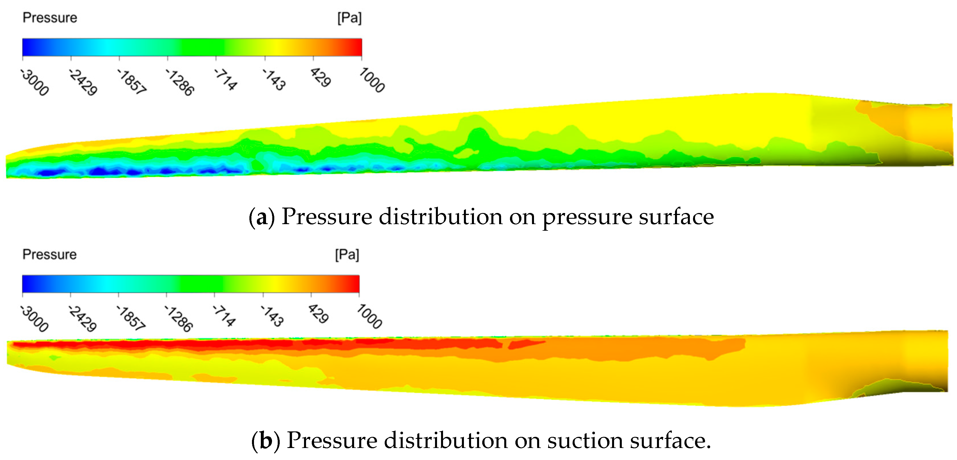
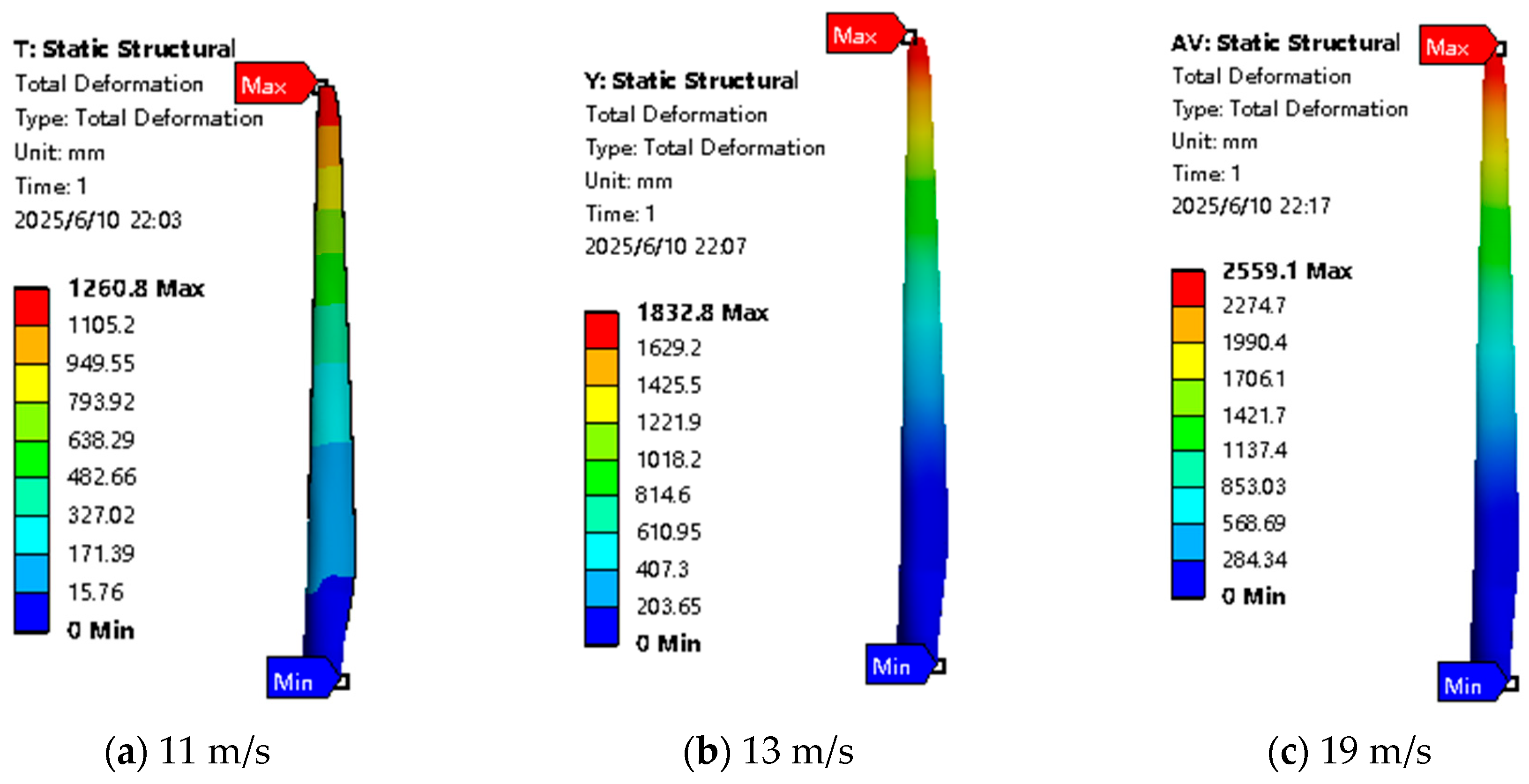
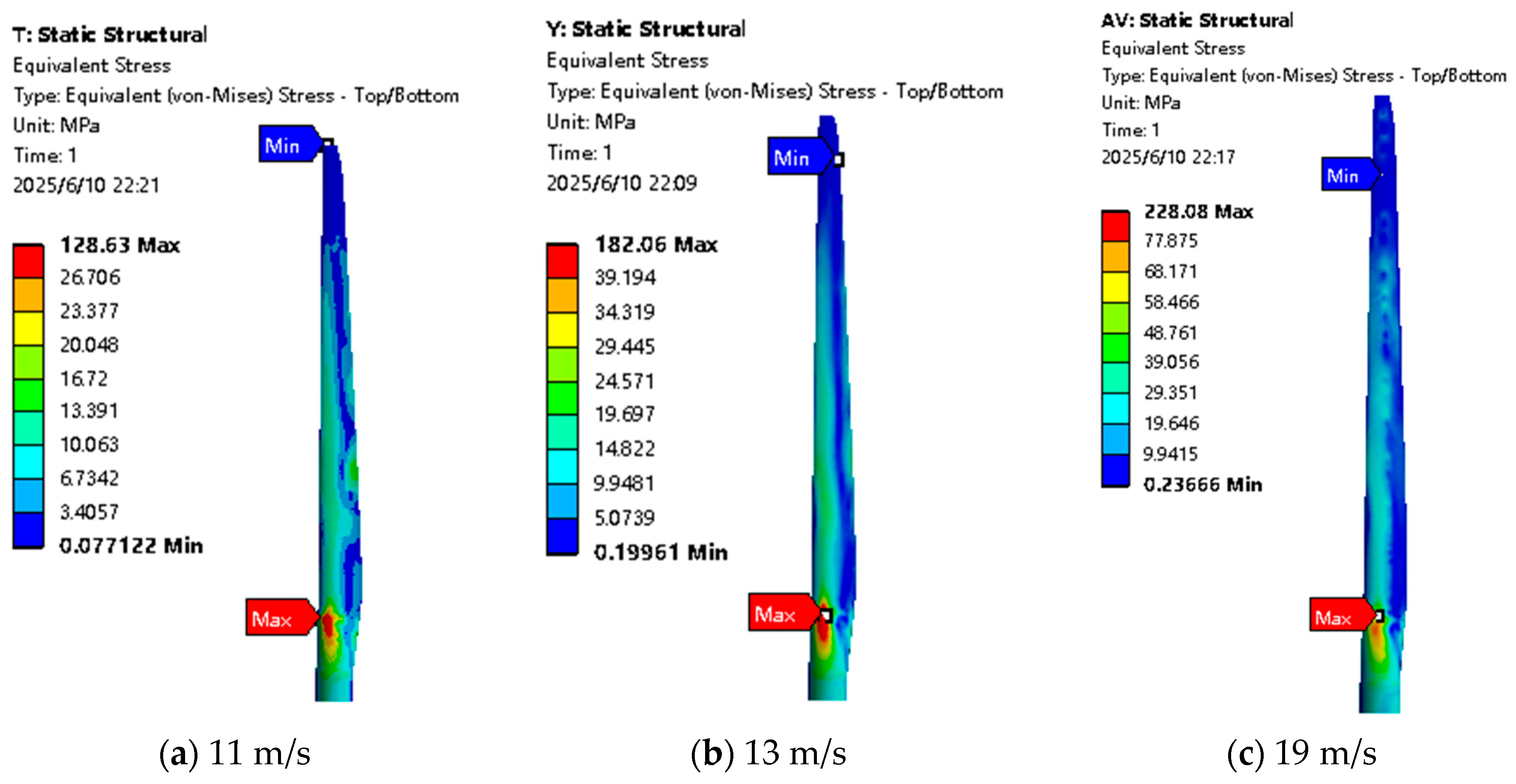
(2) The pressure difference between the suction surface and the pressure surface of the blade drives the fan blade to rotate. Through analysis, the maximum pressure of the blade is located at the transition position between the blade root and the aerodynamic part, and the maximum deformation is situated at the tip of the blade.

(3) The fatigue life of the wind turbine blade estimated based on the fuzzy theory is closer to the actual value than the estimation results of the classical theory, and the life estimation results show that the wind turbine blade can reach its design life.

In this paper, when predicting the fatigue life of the blade, only the normal operating conditions of the wind turbine are considered, and the influence of special conditions such as normal shutdown and emergency shutdown on the fatigue life of the blade is not considered. In future research, the proportion of various working conditions per unit time should be counted, and the damage under the corresponding working conditions should be calculated to make the estimated fatigue life closer to the real situation. Additionally, due to the computer’s performance, the model preprocessing used in this case is not sufficiently fine. In future research, it will be necessary to utilize a composite material layer model that closely resembles the real blade.

References

1. 2024 China Wind Power Hoisting Capacity Statistics Briefing. Wind Energy 2025, 3, 48–63.
2. Aghajani, S.; Hemati, M.; Torabnia, S. Life prediction of wind turbine blades using multi-scale damage model. J. Reinf. Plast. Compos. 2021, 40, 644–653. [Google Scholar] [CrossRef]
3. Kou, H.; An, Z.; Ma, Q.; Guo, X. Lifetime Prediction of Wind Turbine Blade Based on Full-Scale Fatigue Testing. J. Shanghai Jiaotong Univ. (Sci.) 2020, 25, 755–761. [Google Scholar] [CrossRef]
4. Qin, Z. Study on Fatigue Life of Wind Turbine Blades Considering Joint Probability Distribution of Wind Speed and Direction. Doctoral Dissertation, Xinjiang University, Ürümqi, China, 2022. [Google Scholar]
5. Han, T. Research on Structural Damage Diagnosis and Fatigue Life Prediction of Large Wind Turbine Blade. Master’s Thesis, Qingdao University of Science and Technology, Qingdao, China, 2021. [Google Scholar]
6. Zhang, Z. Residual Fatigue Life Analysis of Wind Turbine Blade Based on Damage. Master’s Thesis, Inner Mongolia University of Science & Technology, Baotou, China, 2021. [Google Scholar]
7. Ma, H.; Bi, J.; Ge, X.; Zhou, D.; Jiao, J.; Wang, G. Service Life Prediction of Wind Turbine Blade Based on Optimizated Constant Life Fatigue Limit Model. Acta Energiae Solaris Sin. 2023, 44, 362–369. [Google Scholar]
8. Yu, F. Study on Fatigue Damage Mechanism and Life Prediction of Wind Turbine Blade under Random Loading. Doctoral Dissertation, Shenyang University of Technology, Shenyang, China, 2022. [Google Scholar]
9. Zhao, W.; Zu, J.; Liu, C. Residual strength and life prediction of composites based on static strength distribution parameters. Chin. J. Comput. Mech. 2024, 41, 270–274. [Google Scholar]
10. Epaarachchi, J.A.; Clausen, P.D. The development of a fatigue loading spectrum for small wind turbine blades. J. Wind. Eng. Ind. Aerodyn. 2006, 94, 207–223. [Google Scholar] [CrossRef]
11. Zhang, J. Fatigue Life Prediction of Wind Turbine Blade. Master’s Thesis, Jilin University, Changchun, China, 2013. Available online: https://kns.cnki.net/kns8s/defaultresult/index?crossids=YSTT4HG0%2CLSTPFY1C%2CJUP3MUPD%2CMPMFIG1A%2CWQ0UVIAA%2CBLZOG7CK%2CPWFIRAGL%2CEMRPGLPA%2CNLBO1Z6R%2CNN3FJMUV&korder=SU&kw=%E9%A3%8E%E5%8A%9B%E6%9C%BA%E5%8F%B6%E7%89%87%E7%96%B2%E5%8A%B3%E5%AF%BF%E5%91%BD%E4%BC%B0%E7%AE%97%E6%96%B9%E6%B3%95%E7%A0%94%E7%A9%B6 (accessed on 17 June 2025).
12. Chao, H. Offshore Wind Farms Reliability Evaluation and Repair/Maintenance Resources Optimization Considering Severe Weather Conditions. 2019. Available online: https://kns.cnki.net/kcms2/article/abstract?v=i7m15r_oBqpXt1fyXCIkihYmUoMybVbLVJWXevLpdWj_3amn2lF2L9e1ySbUw_igOEx-R9nzR9kuvx8Tblg2yBnPRzB6m3VQ8Q1VbQPqL9dHmpLl-WY4R_eY-05cdHPs3k2ZLZn49wcXUkd_rDWC1yj5RqIDOOunk9xsLNyX-ZMHsuoXgqtm3cEt8Wk2H0Qh&uniplatform=NZKPT&language=CHS (accessed on 17 June 2025).
13. Li, J.; Zhang, H.; Pang, J. Medium-term and Long-term Wind Speed and Power Generation Forecast Based on Neural Network and Pattern Recognition. Environ. Technol. 2021, 39, 219–226. [Google Scholar]
14. Global Modeling and Assimilation Office (GMAO). MERRA-2 tavg1_2d_lnd_Nx, tavg1_2d_rad_Nx, tavg1_2d_slv_Nx: 2d,1-Hourly, Time-Averaged, Single-Level, Assimilation, Diagnostics V5.12.4 (M2T1NXSLV), Land Surface Diagnostics V5.12.4 (M2T1NXLND), Radiation Diagnostics V5.12.4 (M2T1NXRAD), Greenbelt, MD, USA, Goddard Earth Sciences Data. 2022. Available online: https://xihe-energy.com/ (accessed on 16 June 2025).
15. Wang, S.; Teng, W.; Wang, L.; Liu, Y.; Peng, D.; Ma, Z.; Liu, Y. Modeling of Blade Vibration Mechanism at Edgewise and Flapwise in Horizontal Axis Wind Turbines. J. Mech. Eng. 2024, 60, 131–142. [Google Scholar]
16. Zuo, W.; Li, H.; Rui, X.; Wang, X. Numerical Simulation of Aerodynamic Performance of NREL 5 mw Wind Turbine. Acta Energiae Solaris Sin. 2018, 39, 2446–2452. [Google Scholar]
17. Xu, R.X.; Gao, J.X.; Wu, Z.F. Prediction of Fatigue Life Based on Fuzzy Mathematics and Grey System Theory. J. Mech. Strength 2023, 45, 1452–1458. [Google Scholar]
18. Liang, M.; Nie, G.L.; Cheng, H. Equivalent Load Calculation and Load Spectrum Analysis of Wind Turbine Blade. Mach. Des. Manuf. 2017, 3, 141–143. [Google Scholar]
Figure 1. Technology roadmap.
Processes 13 01951 g001
Figure 2. Flowchart of wind speed simulation method based on MCMC.
Processes 13 01951 g002
Figure 3. Wind field measured wind speed samples.
Processes 13 01951 g003
Figure 4. Comparison of original wind speed and predicted wind speed in 2021.
Processes 13 01951 g004
Figure 5. 3D model of blades.
Processes 13 01951 g005
Figure 6. Calculation domain setting of fan blade.
Processes 13 01951 g006
Figure 7. Pressure distribution on blade surface under rated wind speed.
Processes 13 01951 g007
Figure 8. The total deformation cloud map of the blade.
Processes 13 01951 g008
Figure 9. Equivalent stress cloud diagram of the blade.
Processes 13 01951 g009
Figure 10. The wind speed and stress corresponding to the time series.
Processes 13 01951 g010
Figure 11. Histogram of amplitude and frequency of occurrence.
Processes 13 01951 g011