Data-Driven Prediction of Crystal Size Metrics Using LSTM Networks and In Situ Microscopy in Seeded Cooling Crystallization

Abstract

This work presents a data-driven modeling framework for predicting image-derived crystal size metrics in seeded cooling crystallization using Long Short-Term Memory (LSTM) neural networks. The model leverages in situ microscopy data to predict square-weighted D10, D50, D90, and particle counts based solely on seed loading and temperature profiles, without requiring real-time supersaturation measurements. To enhance predictive power, engineered process descriptors—including temperature derivatives and integrals—were incorporated as dynamic features. Experimental validation was performed using creatine monohydrate crystallization from aqueous solution, with LSTM models trained on a diverse dataset encompassing variable seed loadings and cooling profiles. The feature-engineered LSTM model consistently outperformed its non-engineered counterpart, particularly under nonlinear cooling conditions where crystallization dynamics were the most complex. This approach offers a practical alternative to mechanistic models and spectroscopic process analytical technology (PAT) tools by enabling accurate prediction of chord length distribution (CLD) metrics from routinely collected data. The framework is easily transferable to other crystallization systems and provides a low-complexity, high-accuracy tool for accelerating lab-scale crystallization development.

1. Introduction

Crystallization is a key process in various industries, especially in pharmaceuticals, where control of particle size distribution is essential in ensuring product quality and optimal drug performance, including dissolution profiles [1,2,3]. Particle size distribution not only has a significant impact on the quality of the final product, but also on the efficiency of downstream operations, such as filtration, washing, and drying [4]. The ability to predict and optimize particle size distribution under different process conditions is crucial for ensuring consistent product quality, process efficiency, and scale-up feasibility [5,6,7].

Crystallization modelling plays a crucial role in shortening development times as it provides a predictive framework that minimizes the need for labor-intensive and time-consuming experimental trials [8]. By simulating the effects of process variables on particle size distribution, the models enable rapid iteration during the early development phase, allowing researchers to quickly determine optimal operating conditions [9]. This predictive capability accelerates decision making, particularly in the design and optimization of cooling profiles, seeding strategies, and other critical parameters [10].

Mechanistic approaches such as population equation models (PBEs) are traditionally used to simulate crystallization dynamics, including nucleation, growth, agglomeration, and crystal breakage [10,11,12,13,14]. These models provide fundamental insights into crystallization behavior and have been successfully used in optimizing process conditions [15]. Although mechanistic models can be used for in silico experimentation, accurately determining kinetic parameters requires extensive experimental data to decouple individual crystallization mechanisms [16]. However, PBEs are highly dependent on accurate supersaturation measurements, as supersaturation directly governs nucleation and growth kinetics [17]. Process analytical technologies (PATs) such as attenuated total reflectance Fourier transform infrared spectroscopy (ATR-FTIR) [18,19,20,21,22], Raman spectroscopy [23,24], and attenuated total reflectance ultraviolet–visible spectroscopy (ATR-UV/Vis) [25,26,27,28,29] are commonly used to monitor solution concentration and supersaturation. However, these instruments often require calibration models and chemometric methods to achieve satisfactory accuracy, which can be time- and resource-consuming [30].

To bypass the need for direct supersaturation monitoring, data-driven machine learning (ML) approaches have gained attention for their ability to predict crystallization behavior based on easily measurable process variables [31,32]. Unlike mechanistic models, ML-based methods do not require explicit knowledge of underlying kinetics and instead learn patterns directly from experimental data [33].

Table 1. Summary of examples on mechanistic and machine learning models for crystallization modeling.

Reference	Authors	Problems Addressed	Solving Method
[34]	Y. Liu et al.	Model for cooling crystallization of carbamazepine	PBE
[11]	T. Le Minh et al.	Model for crystallization of L-Lactide in a mixture of n-Hexane and Tetrahydrofuran	PBE
[17]	L. Bosetti et al.	Model of crystal growth and secondary nucleation by attrition and ripening	PBE
[16]	Y. Ma et al.	predicting the final yield and particle size distribution (PSD) in cooling crystallization processes.	ANN
[35]	K. Vasanth Kumar et al.	Model for the crystal growth rate of sucrose	ANN
[36]	B. W. Nyande et al.	Model isothermal crystallization of lysozyme in a batch stirred tank and cooling crystallization of paracetamol	Sparse identification of nonlinear dynamics (SINDy)
[31]	Y. Zheng et al.	Machine-learning-based predictive control schemes for batch crystallization processes	RNN
[37]	F. A. R. D. Lima et al.	Predict the moments of particle-size distribution	Multilayer perceptron (MLP) network, echo state network (ESN), LSTM

provides a summary of examples on mechanistic and machine learning models for crystallization modeling. By including a comparison of different approaches, the table provides a clear overview of the evolution of predictive modeling techniques in crystallization research.

Techniques such as Artificial Neural Networks (ANNs) have been explored in crystallization modeling to extract relationships between process inputs and PSD [16]. However, these models struggle with capturing sequential dependencies, limiting their ability to model time-dependent variations in crystallization.

To address these challenges, this study proposes the use of Long Short-Term Memory (LSTM) networks, a specialized form of recurrent neural networks (RNNs) designed for sequential data processing [38,39]. LSTMs are particularly advantageous for handling time–series data, making them well-suited for predicting PSD in complex crystallization processes where past conditions strongly influence future outcomes [33]. While feedforward neural networks struggle with sequential dependencies, LSTMs leverage memory cells that allow them to retain information over long periods, ensuring that process history is effectively captured [40]. This ability is crucial for modeling nonlinear crystallization dynamics, including variations in cooling profiles. Despite advancements in high-performance computing, solving PBEs remains computationally expensive due to their reliance on numerical solvers for high-dimensional systems, particularly those involving agglomeration and breakage [41]. In contrast, LSTM models, once trained, can rapidly predict PSD evolution without requiring explicit kinetic equations or complex numerical integration.

While alternative RNN architectures such as Gated Recurrent Units (GRUs) and Transformer models have been explored in process modeling applications [40], LSTMs offer a balance between computational efficiency and accuracy. GRUs, although computationally simpler, may not retain long-term dependencies as effectively as LSTMs [42], while Transformer models require large datasets and significant computational resources, making them less practical for crystallization studies with limited data availability [43]. Convolutional Neural Networks (CNNs) have been used for image-based crystallization monitoring but are not well-suited for sequential dependencies inherent in process dynamics [44]. Given these considerations, LSTMs were chosen for their superior ability to capture long-range dependencies in sequential data while remaining computationally feasible for crystallization modeling. While this work applies LSTM networks to predict macroscale crystallization behavior using in situ microscopy data, similar data-driven approaches could also support modeling of kinetic phenomena at the nanoscale [45].

This study explores a data-driven modelling approach that bypasses the need for direct monitoring of supersaturation. Instead, we investigate whether predictive models can be developed by using easily measurable variables such as temperature and seed loadings, in conjunction with real-time particle chord length distribution data. In this context, in situ microscopy plays a central role as it provides high-resolution, real-time insights into the evolution of particle size during the crystallization process [46]. By utilizing advanced techniques such as dark-field illumination, in situ microscopy ensures improved contrast and sensitivity, making it suitable for challenging systems with high dispersed-phase concentrations or small particle sizes [47]. This technology enables the precise measurement of critical metrics, such as the square weighted (SW) D10, D50, D90, and SW counts of the image-derived chord length distribution (ID-CLD), which reflect nucleation and growth dynamics.

Based on this data, we employed Long Short-Term Memory (LSTM) networks, a specialized type of recurrent neural network (RNN) designed to handle time–series data by learning both short- and long-term dependencies. In contrast to conventional machine learning models, LSTMs are able to retain information over longer sequences. This makes them ideal for capturing temporal patterns and dependencies, which are crucial in dynamic processes such as crystallization. This capability is particularly important in scenarios where past conditions strongly influence future outcomes, such as the effects of temperature profiles on particle size distribution.

In this study, the LSTM model utilized lagged inputs derived from the temperature profiles T(t) and seed loading, together with engineered features such as temperature derivatives. These dynamic descriptors provided a comprehensive representation of the process variables and enabled the model to effectively capture the intricate and time-dependent relationships inherent in crystallization dynamics. Using this approach, the LSTM model was able to accurately predict the ID-CLD metrics (SW D10, D50, D90, and SW counts) even under complex and nonlinear process conditions.

The results demonstrate the potential of LSTM models to provide robust predictions of ID-CLD and crystallization dynamics with minimal inputs. By utilizing in situ microscopy data and dynamic process descriptors, the feature-engineered LSTM model showed improved prediction accuracy, especially under dynamic conditions such as nonlinear cooling profiles. These results underline the importance of dynamic features for improving the generalization and adaptability of predictive models and highlight the potential of data-driven approaches.

2. Materials and Methods

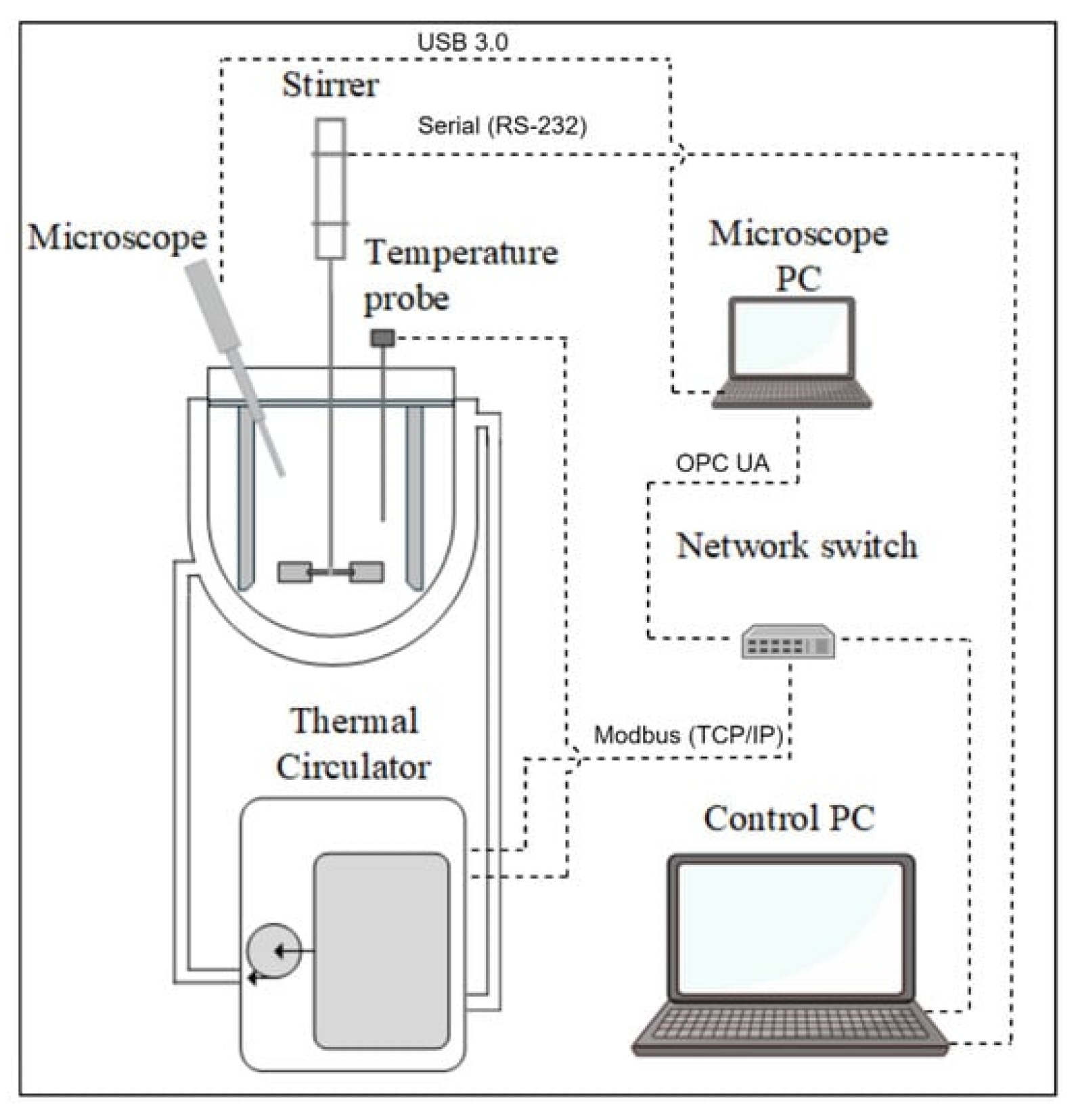
2.1. Experimental Material and Crystallizer Setup

Creatine monohydrate (Polleo Sport, Zagreb, Croatia) and deionized water were selected as the model system for this study. During crystallization from aqueous solution, creatine crystallizes in a monoclinic prism morphology, with each creatine molecule enclosing a water molecule to form the crystalline structure of creatine monohydrate [48,49] (Figure 1).

The experiments were carried out in a jacketed 500 mL glass crystallizer equipped with four flat baffles and a Rushton turbine agitator (Figure 2). The temperature was controlled with a thermostat (Julabo Maggio MS-1000F, Seelbach, Germany), while temperature measurements were recorded with a PTFE-encapsulated Pt-100 sensor (BOLA, Grünsfeld, Germany). The stirring speed was precisely controlled with a stirrer (Heidolph Hei-TORQUE 100, Schwabach, Germany) set to a constant rate to ensure consistent hydrodynamic conditions.

Real-time monitoring of the crystallization process was performed using an in situ microscope (Blaze Metrics LCC Blaze 900 Micro, Bothell, WA, USA) recording ID-CLD metrics. Key features such as SW D10, D50, D90, and SW count were recorded at 5 s intervals along with temperature measurements, providing high-resolution data on crystallization dynamics. A representative image recorded using the in situ microscope is shown in Figure 3. This image highlights typical crystalline morphology during the process.

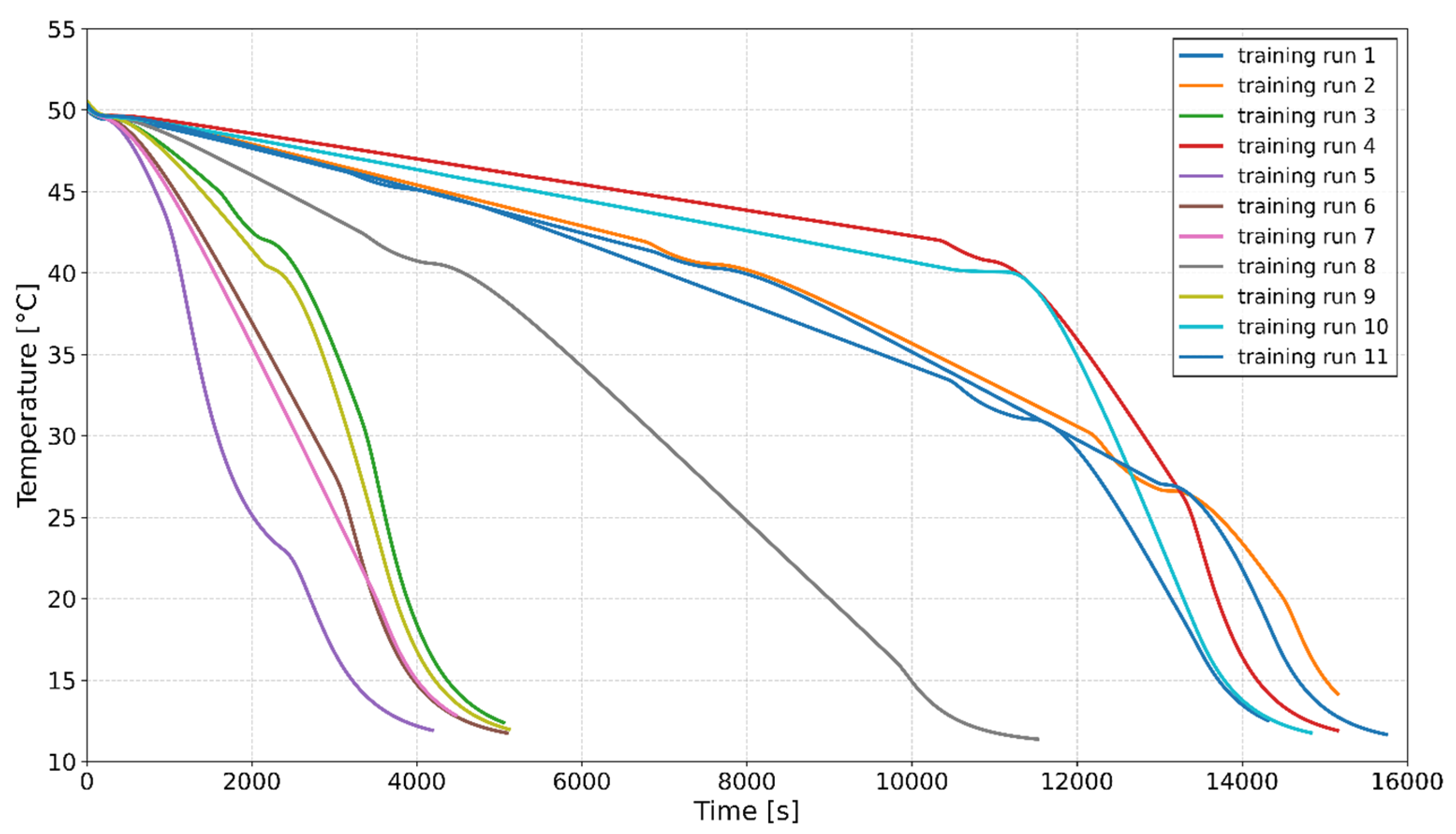
2.2. Crystallization Experiments for Model Training

Crystallization experiments were carried out to generate a comprehensive dataset for training the predictive model. These experiments aimed to capture the variability in crystallization behavior under different process conditions, with a focus on the effects of seed loadings and cooling profiles on ID-CLD. By systematically varying key parameters, the dataset reflects a wide range of operating scenarios and ensures that the model can be effectively generalized under different conditions. A total of 11 experiments were conducted with seed loadings ranging from 0.5% to 3.5%, calculated as:

$$Seed loading, \%={\displaystyle \frac{m_{seed}}{m_{starting mass}}}\ast 100\%$$

(1)

These experiments formed the basis for the development of a robust LSTM-based predictive method capable of capturing the dynamics of cooling crystallization. The training runs were performed with the following seed loadings.

• 0.5% Seed Loading: Training Runs 1, 3, 4, 6, 11
• 2% Seed Loading: Training Runs 2, 7, 8, 9, 10
• 3.5% Seed Loading: Training Run 5

The seeding temperature and concentration were consistently set at 50 ± 0.2 °C and 50 g/L, while the final temperature was 12 ± 2 °C. The stirring rates were maintained at 300 rpm throughout the experiments. To ensure that the dataset captured a wide range of process dynamics, the cooling profiles, shown in Figure 4, were designed to include different patterns. These variations provide a solid basis for training the predictive model.

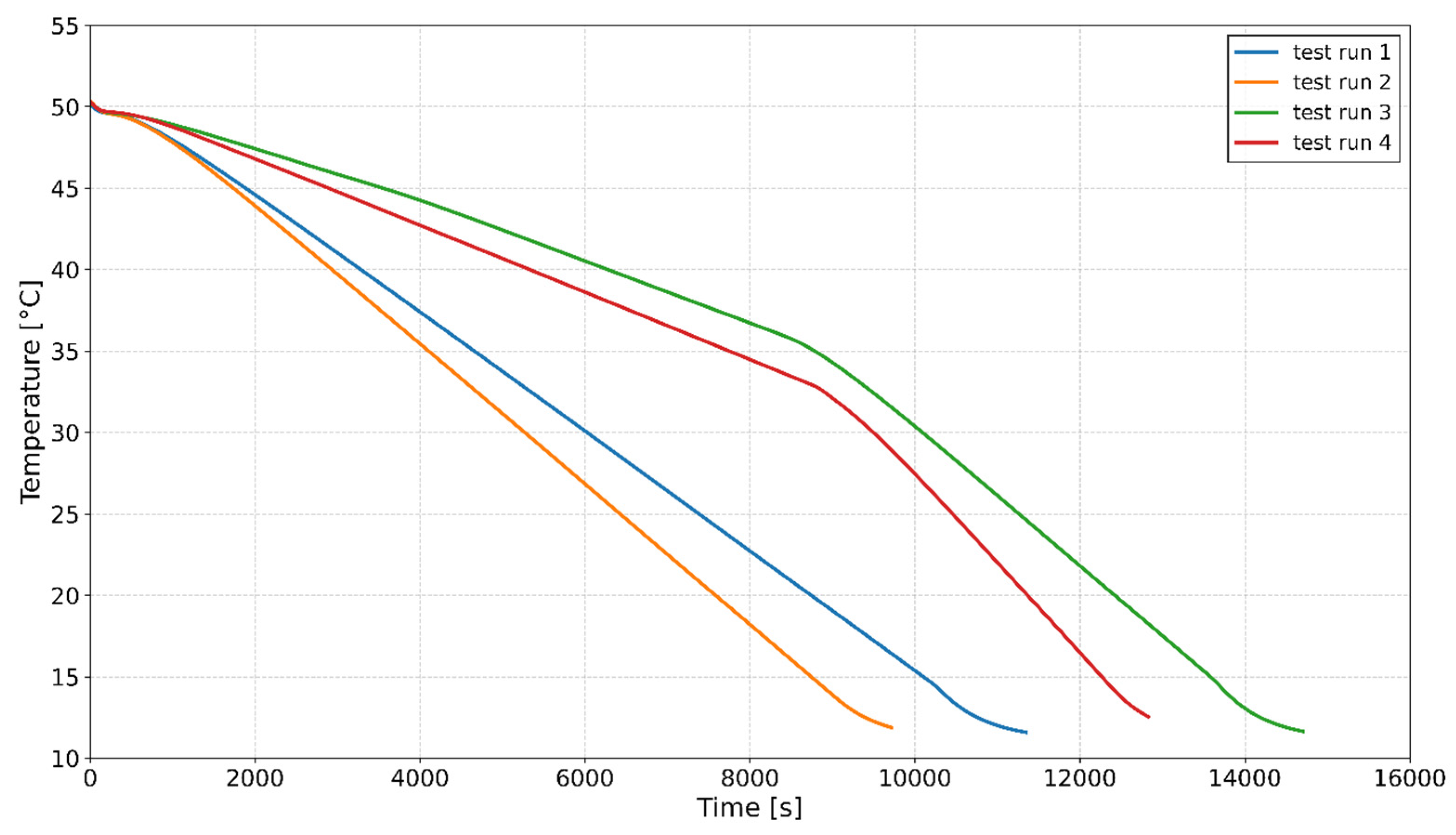
2.3. Crystallization Experiments for Model Testing

To test the models, an additional series of experiments was conducted to evaluate the predictive performance of the trained models under different conditions. The seeding and final temperatures, initial concentration, and stirring rate were kept consistent with those of the training experiments to ensure comparability. Seed loadings (

Table 2. Seed loadings for test runs.

Test Run	1	2	3	4
Seed Loading (%)	1.2	2.5	3	0.75

) between 0.75% and 3.0% were selected to test the developed models under different scenarios.

The cooling profiles used in the test phase (Figure 5) were deliberately designed to differ from the profiles used in training and to introduce new dynamic behaviors. These included a linear cooling profile, rapid cooling conditions, and two nonlinear cooling profiles that allowed a thorough assessment of the model’s ability to generalize in different cooling scenarios.

2.4. Model Building

The predictive modelling framework was developed to capture dynamic relationships within the crystallization process by integrating lagged input steps, data scaling, feature engineering, and Long Short-Term Memory (LSTM) networks. The lagged input variables included temperature, seed loading, and temperature-derived dynamic features. The output variables included the SW counts and SW D10, D50, and D90, which are important process characteristics. To ensure consistency and improve the performance of the model, the input and output variables were normalized using a MinMax scaler. By enriching the dataset with dynamic temperature descriptors, the model’s ability to capture complex relationships was improved. The predictive model was created using an LSTM neural network, which has the ability to learn temporal dependencies and long-term patterns in time–series data, making it particularly suitable for modelling crystallization processes. Hyperparameter optimization was performed using grid search and k-fold cross-validation for both the feature-based and non-feature-based models. The best configurations in each case were compared with an independent test set to ensure robust performance evaluation on unseen data. The implementation was performed in Python (version 3.11) using the PyTorch (version 2.0), Scikit-learn (version 1.2), Pandas (version 1.5), and Numpy (version 1.25) libraries.

2.4.1. Data Scaling

To ensure consistent scaling of the features in the dataset, a MinMax scaler was used.

$$x_{scaled}={\displaystyle \frac{x_i-x_{min}}{x_{max}-x_{min}}}$$

(2)

This preprocessing step was particularly useful for normalizing temperature, seed loading, and ID-CLD features spanning different numerical ranges, improving model performance. By scaling each feature to the range between its minimum (0) and maximum (1) values, the MinMax scaler preserved the relative magnitudes and relationships between the features while preventing any single feature from dominating the analysis due to differences in scale [50]. In this study, seed loading, temperature data, and ID-CLD features were scaled individually. This ensured compatibility with machine learning models such as LSTM, which are sensitive to feature magnitudes.

2.4.2. Feature Engineering from Temperature Profile

In order to capture the dynamic behavior of the cooling process, additional features were derived from the temperature profile T(t). These include the first derivative (dT/dt), which represent the rate of temperature change, the second derivative ($d^{2}T/d{t}^2$), which indicates the acceleration or deceleration of cooling, and the cumulative integral ($\int dT/dt$), which reflects the total temperature change during cooling crystallisation.

The first derivation provided valuable insights into the cooling rate by revealing abrupt changes or steady-state phases. The second derivative provided a deeper understanding of inflection points and transitions by capturing shifts in the cooling trajectory. The cumulative integral quantified the overall temperature change during the process.

By including these features, the dataset was enriched with meaningful descriptors of the cooling process, allowing the predictive model to capture the complex relationships between temperature dynamics and their effects on the crystallization process.

The models were developed both with and without feature engineering to assess their impact on the predictive performance of the models.

2.4.3. LSTM Model—Hyperparameter Optimization

To improve the performance of the LSTM models in predicting the process output, a systematic hyperparameter tuning strategy was applied. This involved a combination of grid search and k-fold cross-validation to evaluate the performance of the model across a range of configurations to ensure robustness and generalization ability. During training, the models were optimized using the Adam optimizer [51] with a fixed learning rate of 5 × 10⁻⁴. This learning rate was chosen to establish a balance between convergence speed and stability during gradient descent.

Grid search was used to comprehensively explore the hyperparameter space for feature-engineered and non-feature-engineered architectures.

The tested parameters included thefollowing:

• Hidden units: the number of hidden units in the LSTM layers (32, 64, 96).
• Number of layers: the number of stacked layers (2, 3).
• Lag: the number of the time steps included in the input sequence (24, 46, 60).

To prevent overfitting and improve generalization, both L1 and L2 regularization techniques were used. L1 regularization, with a strength of 1 × 10⁻⁶, promoted sparsity in the model weights by penalizing their absolute values. L2 regularization, incorporated as a weight decay with a strength of 1 × 10⁻⁶, helped to mitigate overfitting by discouraging excessively large weight values.

A 5-fold cross-validation approach was implemented for the LSTM models to evaluate the performance of each hyperparameter configuration. The dataset was divided into five subsets, with four subsets used for training and the remaining subset reserved for validation. This process was repeated five times, so that each subset served as a validation set once. The average validation loss across all folds was recorded as the primary metric for model evaluation.

The optimization process involved stopping early to prevent overfitting. Training was halted if the validation loss did not improve in 10 consecutive epochs. For each hyperparameter configuration, the validation loss, measured as mean squared error (MSE), was averaged over all output variables and folds. The scaling ensured that all output variables were on the same scale, providing a consistent evaluation metric. The best-performing configuration for the feature-engineered and non-feature-engineered model was selected based on the lowest average MSE value.

$$\mathrm{M}\mathrm{S}\mathrm{E}={\displaystyle \frac{1}{n}}\sum _{i=1}^n{{(y}_i-{\widehat{y}}_i)}^2$$

(3)

After optimizing the architecture, the best-performing configurations for LSTM models with and without features were used for the prediction of the test experiments. The predictive performance of each model was evaluated using the Median Absolute Error (MedAE) and Root Mean Squared Error (RMSE), both calculated for each variable. MedAE was chosen for its robustness to outliers [52,53], while RMSE provides a measure that penalizes larger errors more strongly, making it useful for assessing overall prediction accuracy [54].

$$\mathrm{M}\mathrm{e}\mathrm{d}\mathrm{A}\mathrm{E}=median(\left|y_i-{\widehat{y}}_i\right|,\dots ,\left|y_n-{\widehat{y}}_n\right|)$$

(4)

$$\mathrm{R}\mathrm{M}\mathrm{S}\mathrm{E}=\sqrt{{\displaystyle \frac{1}{n}}\sum _{i=1}^n{(y_i-{\widehat{y}}_i)}^2}$$

(5)

3. Results and Discussion

3.1. Variability in SW D10, D50, D90, and SW Counts Across Crystallization Training Runs

The variations in ID-CLD metrics (SW D10, D50, D90, and SW counts) observed during the training runs are influenced by key input variables: seed loadings and cooling profiles. These differences highlight the complexity of the crystallization process and the need for a robust model to predict results and optimize operating conditions.

Figure 6a–c shows the evolution of the SW D10, D50, and D90 values derived from ID-CLD. Of these values, SW D50 is analyzed in detail as it shows the largest changes. The results show that in experiments with the same seed loading (training run 3–run 11 and run 8–run 10), a slower cooling rate promotes crystal growth by allowing existing crystals to grow instead of initiating nucleation.

Figure 6d shows the evolution of the SW counts, corresponding to the nucleation events. The highest nucleation rate is observed in training run 5, which is characterized by the fastest cooling rate and a high seed loading (3.5%).

The SW counts exhibit clear dependence on the seed loading:

• Training runs 3 and 11 (0.5% seed loading) show the lowest SW counts, which is due to the limited nucleation sites.
• Training runs 8 and 10 (2% seed loading) show intermediate SW counts, which is due to an increase in nucleation events.
• Training run 5 (3.5% seed loading) achieves the highest SW counts, which is due to the fact that a larger seed load provides more nucleation sites and a high degree of supersaturation throughout the process due to the rapid cooling profile.

The results also illustrate the role of cooling rates. For example, the altered cooling profile in training run 10 leads to increased nucleation, which is reflected in higher SW counts and a decrease in SW-D50 values. These results are consistent with crystallization theory, which states that higher supersaturation promotes nucleation, while lower supersaturation facilitates crystal growth.

The dependence of nucleation and growth on the seed loading and the cooling rate underlines the complexity of the crystallization process. This complexity makes it difficult to optimize the operating conditions through experimentation alone, underlining the need for a predictive model. Such a model would enable precise control of particle size distribution, improve process efficiency, and shorten development time.

3.2. Evaluation of LSTM Hyperparameters for Feature-Engineered and Non-Feature-Engineered Models

The grid search optimization process was developed to identify the optimal configurations for both feature and featureless LSTM models. This systematic approach examined a wide range of hyperparameters, including the number of hidden units (32, 64, 96), layers (2, 3), and lag times (24, 48, 60). The performance of each configuration was evaluated using Avg Val Loss, measured as MSE over all scaled output variables. The results of the grid search are summarized in Figure 7.

Feature-engineered models consistently showed lower Avg Val Loss compared to non-feature-engineered models for most configurations, emphasizing the benefits of including dynamic process descriptors. The best-performing feature-engineered configuration achieved an Avg Val Loss of 2.68 × 10⁻³ with 64 hidden units, 3 layers and 60 lag steps. This result highlights the ability of feature engineering to capture complex temporal relationships in the crystallization process. Interestingly, the optimal configuration for the models without feature-engineered models had 96 hidden units, 2 layers and 48 lag steps and achieved an Avg Val Loss of 2.57 × 10⁻³. While this configuration performed better than the feature-engineered counterpart in this particular case, the general trend suggests that feature engineering provides more robust performance over a wider range of hyperparameters.

To further evaluate the ability of the models to generalize beyond the training data, four independent test runs were conducted under different input conditions, including different seed loadings and cooling profiles. These test runs represented different scenarios to evaluate the predictive accuracy and robustness of the models across a range of crystallization dynamics. For this evaluation, the best-performing models identified during the grid search, both with and without feature engineering, were selected to assess the impact of feature engineering on model performance in independent datasets.

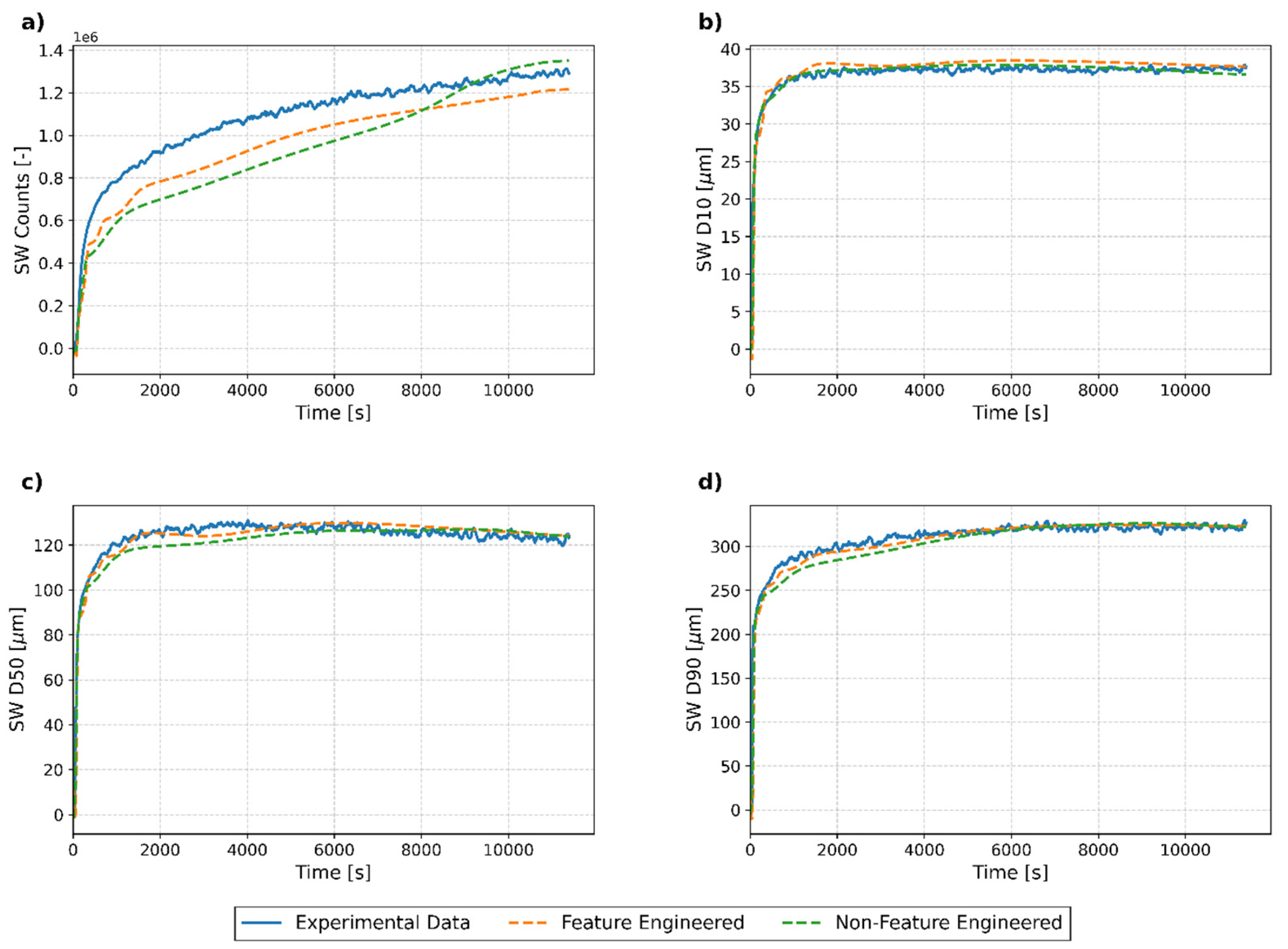
3.3. Analysis of Model Performance Across Test Runs

3.3.1. Overview of Results

In this study, the predictive performance of the LSTM model with and without feature engineering was investigated in four independent test runs, each characterized by different crystallization conditions. The main results, including SW counts, SW D10, D50, and D90, were evaluated to assist our understanding of the ability of the models to generalize under different seed loadings and cooling profiles. The overall results are summarized in

Table 3. MedAE and RMSE comparison for feature-engineered (FE) and non-feature-engineered (NFE) LSTM models.

Run	Variable	MedAE (FE)	MedAE (NFE)	RMSE (FE)	RMSE (NFE)
Test Run 1	SW counts/105	1.17	1.86	1.23	1.73
	SW D10/µm	0.87	0.40	1.33	0.83
	SW D50/µm	2.27	2.96	3.41	4.36
	SW D90/µm	3.13	5.15	9.61	10.86
Test Run 2	SW counts/105	0.40	0.40	0.63	0.71
	SW D10/µm	3.49	4.13	4.01	4.42
	SW D50/µm	8.31	13.11	10.94	14.91
	SW D90/µm	9.68	13.13	17.46	18.99
Test Run 3	SW counts/105	0.20	0.45	0.45	0.61
	SW D10/µm	0.34	2.35	1.56	2.72
	SW D50/µm	1.42	13.35	5.51	13.82
	SW D90/µm	4.17	18.15	10.72	20.06
Test Run 4	SW counts/105	0.92	1.09	1.02	1.10
	SW D10/µm	0.34	1.12	1.72	1.85
	SW D50/µm	2.23	5.78	6.28	7.95
	SW D90/µm	4.09	8.67	15.10	15.47

, which shows the MedAE and RMSE for both models across all test runs. Overall, the feature-engineered model with lower MedAE and RMSE performed better on all ID-CLD metrics.

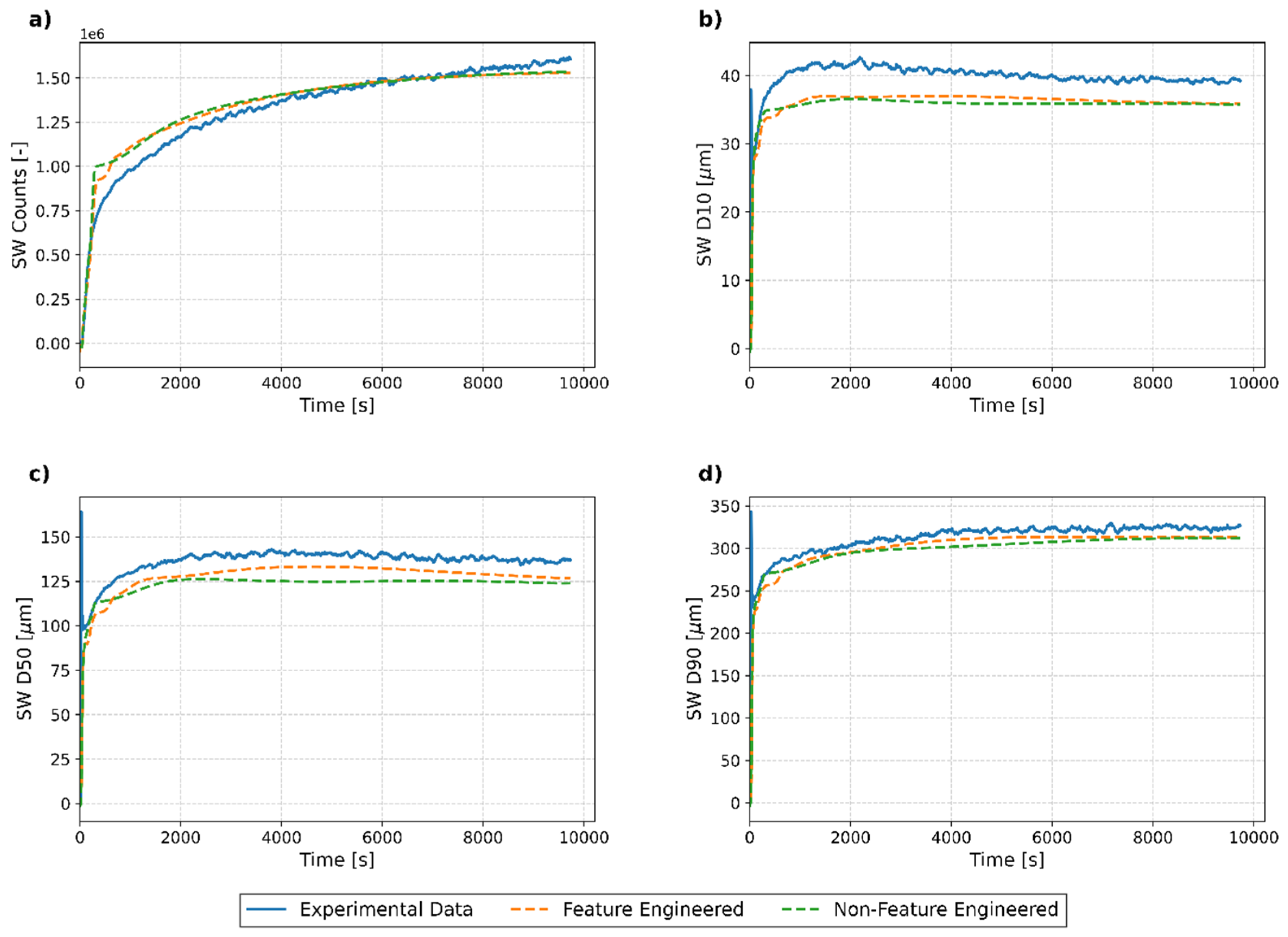
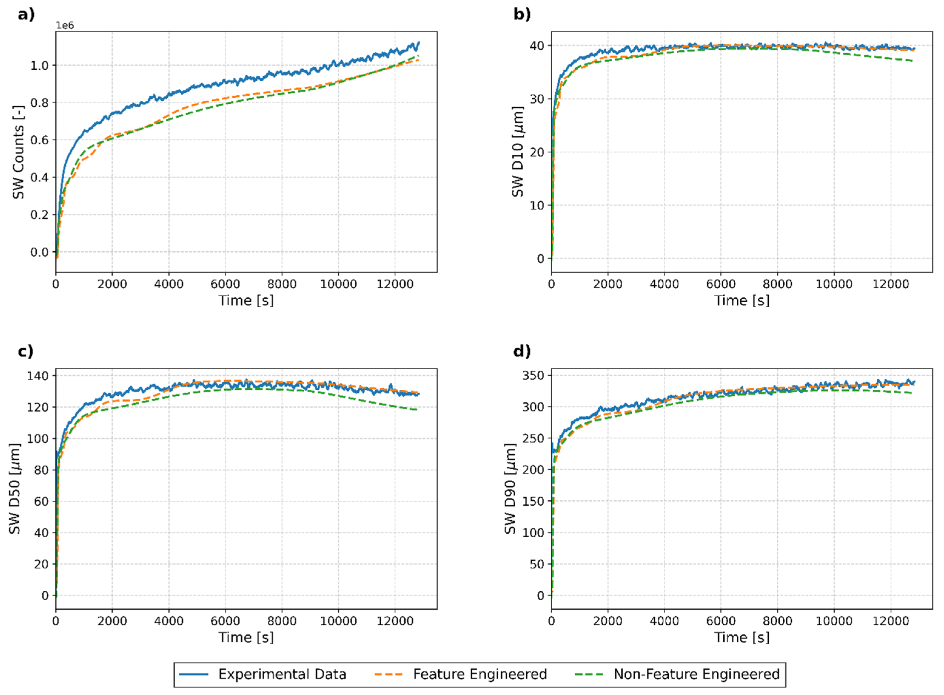
3.3.2. Individual Run Analysis

Test Run 1

Test run 1, defined by a linear cooling profile and a seed loading of 1.2%, was used as a test case to evaluate the model performance at a constant cooling rate.

The most significant difference in prediction accuracy between the models was observed in the SW counts, where the feature-engineered model achieved a 37% reduction in MedAE compared to the non-feature-engineered model. As can be seen in Figure 8a, both models underestimated SW counts, but the feature-engineered model followed the experimental data with a lower error and captured the same nucleation profile as observed experimentally. In contrast, the non-feature-engineered model consistently underestimated the SW counts during the first 9000 s and overestimated them towards the end of the process due to a shift in the prediction of the nucleation rate. This deviation illustrates the inability of the model to fully capture the dynamic effects of nucleation. The improvement observed with the feature-engineered model highlights the importance of including dynamic features, such as temperature derivatives, to better model the dynamics of nucleation and improve prediction accuracy.

For SW D10, D50, and D90, the predictions of both models were remarkably similar, with only slight advantages for the feature-engineered model. As shown in Figure 8b–d, both models closely followed the experimental trends, reflecting the stable growth conditions provided by the linear cooling profile.

Test Run 2

In test run 2, which was defined by a 2.5% seed loading and a rapid cooling profile (orange line in Figure 5), the performance of the models was evaluated under conditions of high supersaturation, which promotes nucleation. Both models showed similar prediction trends, but the feature-engineered model showed slightly better accuracy in most metrics. Despite this improvement, both models underestimated the values for SW D10, D50, and D90.

The SW counts (Figure 9a) showed almost identical performances in the models. The similar prediction accuracy for the SW counts indicates that the nucleation dynamics under high-seed-loading conditions are mainly influenced by seeding.

For SW D50, which represents the median particle size, the feature-engineered model achieved a 37% reduction in MedAE compared to the non-feature-engineered model. As can be seen in Figure 9c, the feature-engineered model agreed better with the experimental data and provided slightly better predictions than the non-feature-engineered model. While both models captured the overall trend quite well, the feature-engineered model showed a modest advantage in accuracy.

Test Run 3

Test run 3, which was characterized by a 3.0% seed loading and a nonlinear cooling profile (green line in Figure 5), resulted in different supersaturation rates throughout the crystallization process. These dynamic conditions posed a challenge for the models as they had to adapt to the changing nucleation and growth rates, which differentiated them from the linear and fast cooling profiles of the previous runs.

In the SW counts (Figure 10a), the performance of both models was comparable, similar to test run 2, which also had high seed loading. Both models had limitations in capturing the subtle changes in nucleation rate associated with the change in cooling rate, resulting in a slight underestimation of SW counts in the later stages of the process.

The feature-engineered model showed clear advantages in predicting SW D50 and SW D90 (Figure 10c,d), which emphasizes its effectiveness in incorporating dynamic features. For SW D90, the feature-engineered model achieved a 77% reduction in MedAE compared to the non-feature-engineered model, closely following the experimental data throughout the process, as can be seen in Figure 10d). Similarly, the feature-engineered model for SW D50 achieved a 90% reduction in MedAE (1.42 vs. 13.33 µm), as seen in Table 3. While the feature-engineered model accurately captured the experimental trends for both metrics, the non-feature-engineered model showed significant underestimates, especially under the influence of the nonlinear cooling profile. These results underline the importance of dynamic features for improving the prediction accuracy of crystallization processes.

The results of test run 3 underline the crucial role of feature engineering in improving the ability of the model to generalize under dynamic crystallization conditions. The nonlinear cooling profile led to transient fluctuations that required the model to adapt to rapid changes in nucleation and growth rates. The feature-engineered model’s ability to incorporate dynamic descriptors such as temperature derivatives and integrals proved essential for the accurate prediction of results such as SW D50 and SW D90, which are influenced by crystal growth and nucleation. These results highlight the limitations of the non-feature-engineered model, which struggled to cope with the variability caused by the nonlinear cooling profile. Overall, test run 3 highlights the effectiveness of the feature-engineered model in accurately capturing the complex crystallization dynamics under nonlinear cooling profiles and demonstrates its robustness and reliability in coping with such challenging process conditions.

Test Run 4

Test run 4, characterized by a seed loading of 0.75% and a nonlinear cooling profile (red line in Figure 5), provided a distinct scenario with a significantly lower seed loading compared to the previous runs. The lower seed loading led to a stronger dependence on solution nucleation and made the process more sensitive to dynamic changes in the cooling rate.

For the SW counts (Figure 11a), both models had difficulty predicting the values accurately, which is due to the low seed loading in test run 4. The reduced seed loading limited the surface area available for crystal growth, resulting in supersaturation in the solution. This increased sensitivity to cooling rates and supersaturation levels added variability in the process and made accurate predictions difficult for both models.

For SW D10, D50, and D90, the feature-engineered model showed better prediction accuracy than the non-feature-engineered model, especially when the cooling rate was changed. As can be seen in Figure 11b–d, the feature-engineered model followed the experimental data for all three metrics—SW D10, D50, and D90—very accurately and successfully captured the transitions caused by the nonlinear cooling profile. In comparison, the non-feature-engineered model had difficulty capturing these transitions, leading to significant deviations in the later stages of crystallization.

3.3.3. Key Findings

Analyzing the effects of seed loading and cooling profiles highlights the unique challenges of each test run and their impact on model performance.

For SW counts, models performed better in runs with higher seed loading (test runs 2 and 3), as sufficient seed loading facilitated crystal growth and minimized variability, reducing dependence on dynamic features. Conversely, in test runs 1 and 4, the surface area available for growth was limited by the low seed loading, resulting in higher MedAE and RMSE.

The results show that feature engineering significantly improves the prediction accuracy of the LSTM models, especially for SW D50 and SW D90 under complex dynamic conditions, such as nonlinear cooling profiles (Test Run 3 and 4). In contrast, for a constant cooling rate, as in test run 1, both models perform similarly for most metrics, with the exception of SW counts.

Overall, the results show the effectiveness of the LSTM models in capturing the dependencies in the seeded cooling. Feature engineering and lagged time steps further improve the model’s capabilities by incorporating process-specific descriptors, enabling more accurate predictions over a wider range of crystallization scenarios.

4. Conclusions

This study investigated the predictive performance of LSTM models for seeded cooling crystallization, focusing on ID-CLD metrics (SW D10, D50, D90, and SW counts). The results show that LSTM models represent the dynamics of crystallization processes very well, whereby the prediction accuracy in complex scenarios is significantly improved by feature engineering.

A key strength of this approach is the ability to achieve accurate predictions without direct monitoring of supersaturation, which is normally required in mechanistic crystallization modelling. Supersaturation, a key factor in nucleation and growth, is often difficult and resource-intensive to measure directly and requires spectroscopy and chemometrics. Instead, the use of lagged data, including seed loading, temperature profile, and its dynamic characteristics, (dT/dt, $d^{2}T/d{t}^2$, $\int dT/dt$) allowed the LSTM model to indirectly capture these dynamics and highlight the effects of previous temperature profiles on crystallization behavior.

The feature-engineered model consistently outperformed the unfeatured model, especially for nonlinear cooling profiles where dynamic variations in growth and nucleation rates were critical. By using dynamic features, such as temperature derivatives and integrals, the feature-engineered model effectively adapted to the changing crystallization conditions and achieved a remarkable reduction in MedAE and RMSE, especially for SW D50 and SW D90.

These results underline the potential of LSTM models as a reliable tool for modelling complex crystallization processes, especially when augmented with feature engineering and lagged input data. By effectively capturing the relationships between process variables and crystallization outcomes without supersaturation measurements, LSTM models reduce the reliance on extensive experimental work and provide valuable opportunities for process simulation and optimization.

Beyond its predictive capabilities, the LSTM model based on in situ microscopy can serve as a valuable tool for identifying optimal crystallization parameters at the laboratory scale. By systematically analyzing the effects of seed loading and cooling profiles, this approach enables us to determine the most effective operating conditions for achieving desired crystal size distributions. These optimized parameters can then be translated to larger-scale production, ensuring consistent product quality while minimizing the need for extensive trial-and-error experimentation during development.

While the LSTM model demonstrated strong predictive capabilities, its application to other crystallization systems remains to be explored. Future studies should assess methodology performance across different solvent systems, hydrodynamic conditions, and active pharmaceutical ingredients (APIs) to evaluate its broader industrial applicability. This framework could also be extended by incorporating additional process variables that play a critical role in other crystallization systems. Additionally, applying this approach to challenging crystallization scenarios, such as needle-like crystal morphologies or systems with high crystal concentrations, remains an important research direction, as accurately extracting chord length distributions (CLD) from in situ microscopy images becomes increasingly difficult under such conditions.

References

1. Zokić, I.; Kardum, J.P. Crystallization Behavior of Ceritinib: Characterization and Optimization Strategies. ChemEngineering 2023, 7, 84. [Google Scholar] [CrossRef]
2. Garg, M.; Rathore, A.S. Process development in the QbD paradigm: Implementing design of experiments (DoE) in anti-solvent crystallization for production of pharmaceuticals. J. Cryst. Growth 2021, 571, 126263. [Google Scholar] [CrossRef]
3. Chen, J.; Sarma, B.; Evans, J.M.B.; Myerson, A.S. Pharmaceutical crystallization. Cryst. Growth Des. 2011, 11, 887–895. [Google Scholar] [CrossRef]
4. Lee, H.L.; Lin, H.Y.; Lee, T. The impact of reaction and crystallization of acetaminophen (Paracetamol) on filtration and drying through in-process controls. In Proceedings of the Particle Technology Forum 2014—Core Programming Area at the 2014 AIChE Annual Meeting, Atlanta, GA, USA, 16–21 November 2014; pp. 275–286. [Google Scholar]
5. Wei, H.Y. Computer-aided design and scale-up of crystallization processes: Integrating approaches and case studies. Chem. Eng. Res. Des. 2010, 88, 1377–1380. [Google Scholar] [CrossRef]
6. Woinaroschy, A.; Isopescu, R.; Filipescu, L. Crystallization process optimization using artificial neural networks. Chem. Eng. Technol. 1994, 17, 269–272. [Google Scholar] [CrossRef]
7. Worlitschek, J.; Mazzotti, M. Model-based optimization of particle size distribution in batch-cooling crystallization of paracetamol. Cryst. Growth Des. 2004, 4, 891–903. [Google Scholar] [CrossRef]
8. Mazzotti, M.; Vetter, T.; Ochsenbein, D.R. Crystallization Process Modeling. In Polymorphism in the Pharmaceutical Industry; Wiley-VCH Verlag GmbH & Co., KGaA: Weinheim, Germany, 2018; pp. 285–304. [Google Scholar] [CrossRef]
9. Pickles, T.; Svoboda, V.; Marziano, I.; Brown, C.J.; Florence, A.J. Integration of a model-driven workflow into an industrial pharmaceutical facility: Supporting process development of API crystallisation. CrystEngComm 2024, 26, 4678–4689. [Google Scholar] [CrossRef]
10. Fiordalis, A.; Georgakis, C. Data-driven, using design of dynamic experiments, versus model-driven optimization of batch crystallization processes. J. Process Control 2013, 23, 179–188. [Google Scholar] [CrossRef]
11. Le Minh, T.; Thanh, T.P.; Hong, N.N.T.; Minh, V.P. A Simple Population Balance Model for Crystallization of L-Lactide in a Mixture of n-Hexane and Tetrahydrofuran. Crystals 2022, 12, 221. [Google Scholar] [CrossRef]
12. Szilagyi, B.; Eren, A.; Quon, J.L.; Papageorgiou, C.D.; Nagy, Z.K. Application of Model-Free and Model-Based Quality-by-Control (QbC) for the Efficient Design of Pharmaceutical Crystallization Processes. Cryst. Growth Des. 2020, 20, 3979–3996. [Google Scholar] [CrossRef]
13. Rosenbaum, T.; Tan, L.; Engstrom, J. Advantages of utilizing population balance modeling of crystallization processes for particle size distribution prediction of an active pharmaceutical ingredient. Processes 2019, 7, 355. [Google Scholar] [CrossRef]
14. Jha, S.K.; Karthika, S.; Radhakrishnan, T.K. Modelling and control of crystallization process. Resour. Technol. 2017, 3, 94–100. [Google Scholar] [CrossRef]
15. Nagy, Z.K.; Braatz, R.D. Advances and new directions in crystallization control. Annu. Rev. Chem. Biomol. Eng. 2012, 3, 55–75. [Google Scholar] [CrossRef]
16. Ma, Y.; Li, W.; Yang, H.; Gong, J.; Nagy, Z.K. Digital Design of Cooling Crystallization Processes Using a Machine Learning-Based Strategy. Ind. Eng. Chem. Res. 2024, 63, 20236–20251. [Google Scholar] [CrossRef]
17. Bosetti, L.; Mazzotti, M. Population Balance Modeling of Growth and Secondary Nucleation by Attrition and Ripening. Cryst. Growth Des. 2020, 20, 307–319. [Google Scholar] [CrossRef]
18. Herceg, T.; Andrijić, Ž.U.; Gavran, M.; Sacher, J.; Vrban, I.; Bolf, N. Application of Neural Networks for Estimating the Concentration of Active Ingredients Solution using In-situ ATR-FTIR Spectroscopy. Kem. Ind. 2023, 72, 639–650. [Google Scholar] [CrossRef]
19. Zhang, F.; Du, K.; Guo, L.; Xu, Q.; Shan, B. Comparative Study of Preprocessing on an ATR-FTIR Calibration Model for In Situ Monitoring of Solution Concentration in Cooling Crystallization. Chem. Eng. Technol. 2021, 44, 2279–2289. [Google Scholar] [CrossRef]
20. Togkalidou, T.; Fujiwara, M.; Patel, S.; Braatz, R.D. Solute concentration prediction using chemometrics and ATR-FTIR spectroscopy. J. Cryst. Growth 2001, 231, 534–543. [Google Scholar] [CrossRef]
21. Togkalidou, T.; Tung, H.H.; Sun, Y.; Andrews, A.; Braatz, R.D. Solution concentration prediction for pharmaceutical crystallization processes using robust chemometrics and ATR FTIR spectroscopy. Org. Process Res. Dev. 2002, 6, 317–322. [Google Scholar] [CrossRef]
22. Lewiner, F.; Klein, J.P.; Puel, F.; Feh, G. On-line ATR FTIR measurement of supersaturation during solution crystallization processes. Calibration and applications on three solute/solvent systems. Chem. Eng. Sci. 2001, 56, 2069–2084. [Google Scholar] [CrossRef]
23. Lin, M.; Wu, Y.; Rohani, S. Simultaneous Measurement of Solution Concentration and Slurry Density by Raman Spectroscopy with Artificial Neural Network. Cryst. Growth Des. 2020, 20, 1752–1759. [Google Scholar] [CrossRef]
24. Gavran, M.; Andrijić, Ž.U.; Bolf, N.; Rimac, N.; Sacher, J.; Šahnić, D. Development of a Calibration Model for Real-Time Solute Concentration Monitoring during Crystallization of Ceritinib Using Raman Spectroscopy and In-Line Process Microscopy. Processes 2023, 11, 3439. [Google Scholar] [CrossRef]
25. Zhang, Y.; Jiang, Y.; Zhang, D.; Li, K.; Qian, Y. On-line concentration measurement for anti-solvent crystallization of β-artemether using UVvis fiber spectroscopy. J. Cryst. Growth 2011, 314, 185–189. [Google Scholar] [CrossRef]
26. Simone, E.; Saleemi, A.N.; Tonnon, N.; Nagy, Z.K. Active polymorphic feedback control of crystallization processes using a combined raman and ATR-UV/Vis spectroscopy approach. Cryst. Growth Des. 2014, 14, 1839–1850. [Google Scholar] [CrossRef]
27. Saleemi, A.N.; Rielly, C.D.; Nagy, Z.K. Monitoring of the combined cooling and antisolvent crystallisation of mixtures of aminobenzoic acid isomers using ATR-UV/vis spectroscopy and FBRM. Chem. Eng. Sci. 2012, 77, 122–129. [Google Scholar] [CrossRef]
28. Billot, P.; Couty, M.; Hosek, P. Application of ATR-UV spectroscopy for monitoring the crystallisation of UV absorbing and nonabsorbing molecules. Org. Process Res. Dev. 2010, 14, 511–523. [Google Scholar] [CrossRef]
29. Vrban, I.; Šahnić, D.; Bolf, N. Artificial Neural Network Models for Solution Concentration Measurement during Cooling Crystallization of Ceritinib. Teh. Glas. 2024, 18, 354–362. [Google Scholar] [CrossRef]
30. Qu, H.; Alatalo, H.; Hatakka, H.; Kohonen, J.; Kultanen, M.L.; Reinikainen, S.P.; Kallas, J. Raman and ATR FTIR spectroscopy in reactive crystallization: Simultaneous monitoring of solute concentration and polymorphic state of the crystals. J. Cryst. Growth 2009, 311, 3466–3475. [Google Scholar] [CrossRef]
31. Zheng, Y.; Wang, X.; Wu, Z. Machine Learning Modeling and Predictive Control of the Batch Crystallization Process. Ind. Eng. Chem. Res. 2022, 61, 5578–5592. [Google Scholar] [CrossRef]
32. Lu, M.; Rao, S.; Yue, H.; Han, J.; Wang, J. Recent Advances in the Application of Machine Learning to Crystal Behavior and Crystallization Process Control. Cryst. Growth Des. 2024, 24, 5374–5396. [Google Scholar] [CrossRef]
33. Sitapure, N.; Kwon, J.S.I. Machine learning meets process control: Unveiling the potential of LSTMc. AIChE J. 2024, 70, 1–18. [Google Scholar] [CrossRef]
34. Liu, Y.; Acevedo, D.; Yang, X.; Naimi, S.; Wu, W.; Pavurala, N.; Nagy, Z.; O’Connor, T. Population Balance Model Development Verification and Validation of Cooling Crystallization of Carbamazepine. Cryst. Growth Des. 2020, 20, 5235–5250. [Google Scholar] [CrossRef]
35. Kumar, K.V.; Martins, P.; Rocha, F. Modelling of the batch sucrose crystallization kinetics using artificial neural networks: Comparison with conventional regression analysis. Ind. Eng. Chem. Res. 2008, 47, 4917–4923. [Google Scholar] [CrossRef]
36. Nyande, B.W.; Nagy, Z.K.; Lakerveld, R. Data-driven identification of crystallization kinetics. AIChE J. 2024, 70, 1–11. [Google Scholar] [CrossRef]
37. Lima, F.A.R.D.; de Miranda, G.F.M.; de Moraes, M.G.F.; Capron, B.D.O.; de Souza, M.B. A Recurrent Neural Networks-Based Approach for Modeling and Control of a Crystallization Process. Comput. Aided Chem. Eng. 2022, 51, 1423–1428. [Google Scholar] [CrossRef]
38. Staudemeyer, R.C.; Morris, E.R. Understanding LSTM—A tutorial into Long Short-Term Memory Recurrent Neural Networks. arXiv 2019, arXiv:1909.09586. [Google Scholar] [CrossRef]
39. Hochreiter, S.; Schmidhuber, J. Long Short-Term Memory. Neural Comput. 1997, 9, 1735–1780. [Google Scholar] [CrossRef]
40. Meyer, C.; Arora, A.; Scholl, S. A method for the rapid creation of AI driven crystallization process controllers. Comput. Chem. Eng. 2024, 186, 108680. [Google Scholar] [CrossRef]
41. Omar, H.M.; Rohani, S. Crystal Population Balance Formulation and Solution Methods: A Review. Cryst. Growth Des. 2017, 17, 4028–4041. [Google Scholar] [CrossRef]
42. Yang, X.; Muhammad, T.; Bakri, M.; Muhammad, I.; Yang, J.; Zhai, H.; Abdurahman, A.; Wu, H. Simple and fast spectrophotometric method based on chemometrics for the measurement of multicomponent adsorption kinetics. J. Chemom. 2020, 34, 1–13. [Google Scholar] [CrossRef]
43. Sitapure, N.; Kwon, J.S.-I. CrystalGPT: Enhancing system-to-system transferability in crystallization prediction and control using time-series-transformers. Comput. Chem. Eng. 2023, 177, 108339. [Google Scholar] [CrossRef]
44. Salami, H.; McDonald, M.A.; Bommarius, A.S.; Rousseau, R.W.; Grover, M.A. In Situ Imaging Combined with Deep Learning for Crystallization Process Monitoring: Application to Cephalexin Production. Org. Process Res. Dev. 2021, 25, 1670–1679. [Google Scholar] [CrossRef]
45. Piskunova, N.N. Non-reversibility of crystal growth and Dissolution: Nanoscale direct observations and kinetics of transition through the saturation point. J. Cryst. Growth 2024, 631, 127614. [Google Scholar] [CrossRef]
46. Mentges, J.; Bischoff, D.; Walla, B.; Weuster-Botz, D. In Situ Microscopy with Real-Time Image Analysis Enables Online Monitoring of Technical Protein Crystallization Kinetics in Stirred Crystallizers. Crystals 2024, 14, 1009. [Google Scholar] [CrossRef]
47. Sacher, J.B.; Bolf, N.; Sejdić, M. Batch Cooling Crystallization of a Model System Using Direct Nucleation Control and High-Performance In Situ Microscopy. Crystals 2024, 14, 1079. [Google Scholar] [CrossRef]
48. Antonio, J.; Candow, D.G.; Forbes, S.C.; Gualano, B.; Jagim, A.R.; Kreider, R.B.; Rawson, E.S.; Smith-Ryan, A.E.; VanDusseldorp, T.A.; Willoughby, D.S.; et al. Common questions and misconceptions about creatine supplementation: What does the scientific evidence really show? J. Int. Soc. Sport. Nutr. 2021, 18, 13. [Google Scholar] [CrossRef]
49. Jäger, R.; Purpura, M.; Shao, A.; Inoue, T.; Kreider, R.B. Analysis of the efficacy, safety, and regulatory status of novel forms of creatine. Amino Acids 2011, 40, 1369–1383. [Google Scholar] [CrossRef]
50. de Amorim, L.B.V.; Cavalcanti, G.D.C.; Cruz, R.M.O. The choice of scaling technique matters for classification performance. Appl. Soft Comput. 2023, 133, 109924. [Google Scholar] [CrossRef]
51. Kingma, D.P.; Ba, J.L. Adam: A method for stochastic optimization. In Proceedings of the 3rd International Conference on Learning Representations, ICLR 2015—Conference Track Proceedings, San Diego, CA, USA, 7–9 May 2015; pp. 1–15. [Google Scholar]
52. Yu, H.; Hu, Y.; Shi, P. A Prediction Method of Peak Time Popularity Based on Twitter Hashtags. IEEE Access 2020, 8, 61453–61461. [Google Scholar] [CrossRef]
53. Hyndman, R.J.; Koehler, A.B. Another look at measures of forecast accuracy. Int. J. Forecast. 2006, 22, 679–688. [Google Scholar] [CrossRef]
54. Chai, T.; Draxler, R.R. Root mean square error (RMSE) or mean absolute error (MAE)?—Arguments against avoiding RMSE in the literature. Geosci. Model. Dev. 2014, 7, 1247–1250. [Google Scholar] [CrossRef]
Figure 1. Molecular structure of creatine monohydrate.
Processes 13 01860 g001
Figure 2. Crystallizer setup [47].
Processes 13 01860 g002
Figure 3. In situ microscopy image collected during crystallization of creatine monohydrate.
Processes 13 01860 g003
Figure 4. Temperature profiles used in training experiments.
Processes 13 01860 g004
Figure 5. Temperature profiles used in test experiments.
Processes 13 01860 g005
Figure 6. Variability in ID-CLD metrics across training runs: (a) SW D10, (b) SW D50, (c) SW D90, and (d) SW counts.
Processes 13 01860 g006
Figure 7. Comparison of Avg Val Loss for LSTM architectures: (a) feature-engineered and (b) non-feature-engineered.
Processes 13 01860 g007
Figure 8. Performance of feature-engineered and non-feature-engineered LSTM models for test run 1: (a) SW counts, (b) SW D10, (c) SW D50, and (d) SW D90.
Processes 13 01860 g008
Figure 9. Performance of feature-engineered and non-feature-engineered LSTM models for test run 2: (a) SW counts, (b) SW D10, (c) SW D50, and (d) SW D90.
Processes 13 01860 g009
Figure 10. Performance of feature-engineered and non-feature-engineered LSTM models for test run 3: (a) SW counts, (b) SW D10, (c) SW D50, and (d) SW D90.
Processes 13 01860 g010
Figure 11. Performance of feature-engineered and non-feature-engineered LSTM models for test run 4: (a) SW counts, (b) SW D10, (c) SW D50, and (d) SW D90.
Processes 13 01860 g011