Abstract
Fibrous biomaterials are essential in biomedical engineering, tissue engineering, and filtration due to their specific transport and mechanical properties. Fluid flow through these materials is critical for their function. However, many biological fluids exhibit non-Newtonian behavior, characterized by micro-rotational effects, which traditional models often overlook. The current study presents a machine learning (ML) framework for the prediction and understanding of hydraulic permeability in fibrous biomaterials with a micropolar fluid. A dataset of 1000 numerical simulations was generated by varying the micropolar fluid properties and the fiber volume fraction in a periodic porous structure with nine parallel cylindrical fibers in a square lattice. Six powerful ML algorithms were deployed: Decision Trees (DT), Random Forests (RF), XGBoost, LightGBM, Support Vector Regression (SVR), and k-Nearest Neighbors (kNN). The balance of predictive capacity to unseen data values (tracking values and error metrics) with computational efficiency for all algorithms was assessed. The best-performing ML algorithm was subsequently used to interpret the decisions made by the model using Shapley Additive exPlanations (SHAP) analysis and understand the role of feature importances. The SHAP findings highlight the potential of ML in capturing complex fluid interactions and guiding the design of advanced fibrous biomaterials with optimized hydraulic permeability.
1. Introduction
Fibrous biomaterials, due to their unique transport and mechanical properties, are widely used in biomedical engineering [1], tissue engineering [2], and filtration applications [3]. Different types of biological fibers are frequently encountered, including collagen fibers, elastin fibers, and fibrin networks [4], as well as synthetic bio-based fibers such as polylactides (PLAs) and polyhydroxyalkanoates (PHAs), produced via electrospinning [4]. These biomaterials have diverse applications: from cell migration wound healing replacement, to the growth of native extracellular matrix and gas permeability [5].
In the above applications, the fluid flow in the open space between the formed fibrous lattice is crucial, and it is of especially high importance in biomedical engineering applications due to the sensitivity of cell structures to mechanical/shear stress as well as micro-scale transport of species such as nutrients, oxygen, CO2, and other metabolic products [6]. In implants and tissue scaffolds, flow in the porous region promotes favorable tissue responses as well as diffusion of oxygen and nutrients [7]. Also, the presence of porosity in nanofiber biomaterials allows for high efficiency in drug storage and release [8]. It can be easily inferred that the permeability of the above-mentioned fibrous biomaterials is highly dependent on their porosity and microstructure, as well as interactions with the surrounding fluid.
It has long been recognized that the flow of biological fluids through fibrous biomaterials deviates from Newtonian behavior. Such complex fluids possess an internal structure, reflected in the movement and orientation of their microscopic constituents. One classic example is blood. It comprises suspended particles such as red blood cells, platelets, and white blood cells in plasma [9]. These constituents can rotate, aside from the possible rotation of the bulk fluid, and interact, leading to micro-rotational effects that cannot be captured by Newtonian models. Another example is synovial fluid, which lubricates the joints and contains microstructures made of hyaluronic acid and other macromolecules [10]. Also, in magnetic hyperthermia of tumors, the colloidal nanofluid contains magnetic nanoparticles (e.g., iron oxides) that can physically rotate due to the application of an external magnetic field [11]. Biofluids that manifest the above-mentioned behavior are frequently referred to as micropolar, the concept of which was first introduced in the foundational study by Eringen [12]. These fluids exhibit a non-symmetric stress tensor and are generally characterized by the asynchrony of their microrotation and the vorticity of the liquid carrier [13,14].
The study of flow through fibrous materials has been an ongoing research field, centered mainly around materials processing. The permeability of fibrous media has been experimentally measured using several techniques [15,16,17]. Theoretical approaches have also been followed, for square and hexagonal fiber arrays, using, for instance, the free-surface model [18], the lubrication approximation [19], and an integral technique [20]. Also, several studies have been carried out to include the effect of size variation and perturbation of the fiber position in unidirectional fiber arrays [21,22,23]. In the above studies, the fluid was assumed to be a Newtonian or generalized-Newtonian fluid. Determining the hydraulic permeability of fibrous biomaterials with a micropolar fluid has been studied far less extensively. Erisken et al. [24], carried out numerical simulations using a micropolar fluid to study the effect of collagen fibril diameter distribution on effective permeability of healthy and injured tissues. Karvelas et al. [25] also used numerical simulations in an effort to identify how the micropolar fluid properties affect the hydraulic permeability in fibrous biomaterials.
Artificial Intelligence (AI) techniques have already exerted a significant impact on various technological areas and are poised to revolutionize both the research and development of materials and processes. Machine learning (ML) has recently emerged as an AI branch focusing on the use of datasets and algorithms for learning patterns, making predictions based on the trained patterns, and progressively improving prediction accuracy with minimal human intervention. A common ML process is supervised learning, typically involving a learning procedure via mapping given input and output pairs. The success of ML and AI techniques in various technological areas is due to the availability of digital (large) datasets. Ideally, the dataset should be created from real-world measurements/observations, the so-called ground truth. For example, Zade et al. [26], in order to construct a training dataset, used sensors and visualization techniques to measure the permeability of reinforcement mats with Newtonian fluids for four input parameters. Subsequently, the obtained experimental data were used by different ML techniques to model the permeability of the mats. Alternatively, numerical simulations for the fluid flow description in the fibrous microstructure can be perceived as the ground truth. In this context, Caglar et al. [27] used deep learning to train several pixelized image microstructures, combined with numerical Newtonian flow simulations, to predict the permeability of the fibrous structures. Moreover, Froning et al. [28] used deep learning methods and numerical flow simulations via the lattice Boltzmann method for a Newtonian fluid to predict the permeability and tortuosity of fibrous gas diffusion layers. Schmidt et al. [29] carried out Newtonian fluid numerical simulations for the generation of datasets for permeability estimation of composite microstructures and subsequently used ML techniques as a surrogate model for the simulations.
Understanding how biological fluids are transported through fibrous biomaterials is essential in many biomedical applications. Since many biological fluids do not typically exhibit Newtonian behavior, the present study constitutes a new ML-based framework to predict how easily such fluids can flow through fibrous structures. While earlier research focused on the permeability of these materials through experiments, theoretical models, and some recent efforts using AI techniques, these efforts were all based on the assumption of Newtonian fluid behavior. The present study takes a different path: it focuses specifically on micropolar fluids, which exhibit micro-rotational effects, and their interaction with the microstructure of fibrous biomaterials.
To achieve this, we created an extensive dataset using numerical simulations that reflect the unique transport properties of micropolar fluids. The goal is to train a surrogate model that not only predicts hydraulic permeability accurately but also does so efficiently. The present ML framework offers a fast and reliable way to analyze fluid transport in fibrous systems, with the aim of advancing the design of biomaterials used in areas like tissue engineering and drug delivery, where understanding fluid flow is critical.
2. Materials and Methods
2.1. Geometry and Dataset Generation
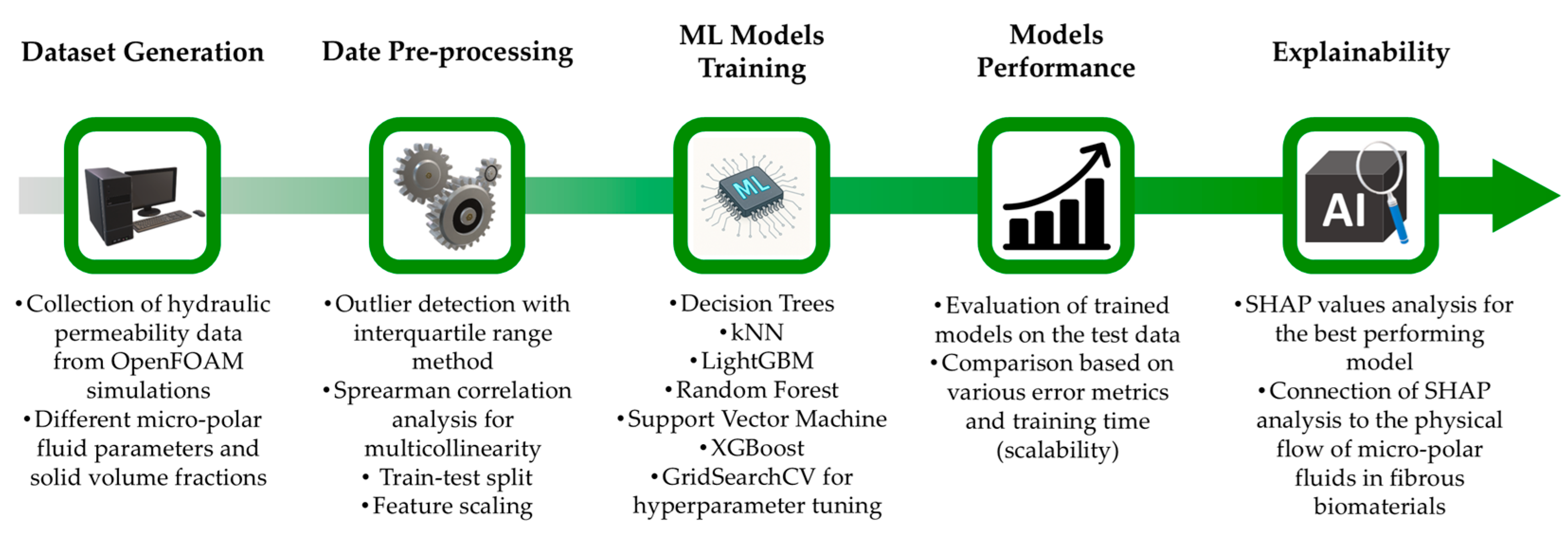
The proposed machine learning framework is shown schematically in Figure 1. There are several steps involved, starting from dataset generation and pre-processing to the use of ML models and interpretation of the best-performing model. For the dataset acquisition, we assume that porous structures of fibrous biomaterials can be replicated using the assembly shown in Figure 2, previously employed in the study by Karvelas et al. [25]. It consists of nine parallel cylindrical fibers in a regular square periodic packing. Several technical details, including micropolar fluid flow equations and numerical simulation setup, were fully disclosed in [25]. In the present study, for completeness, they are briefly summarized. The porous structure in Figure 2 has scaled dimensions , and the solid volume fraction of the structure is given by , where is the dimensionless diameter of the cylindrical fiber.

Figure 1.
Schematic representation of the proposed machine learning (ML) framework.
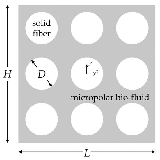
Figure 2.
Schematic representation of the regularly ordered fiber array consisting of nine cylinders, replicating the microstructure of fibrous biomaterials. The micropolar bio-fluid flows between the cylindrical solid fibers.
The material flows due to an applied pressure drop in the x-direction. Under steady-state and incompressible flow conditions, the laminar flow of the micropolar biofluid in the space between the fibers is governed by the following dimensionless equations [9,12,30]
where is the biofluid dimensionless velocity vector, is the dimensionless rotational velocity vector, and is the dimensionless pressure. is the Reynolds number given by
is a non-dimensional parameter known as spin-gradient viscosity
is a dimensionless form of the vortex viscosity given by
and is the dimensionless microinertia
In the above equations, is the fluid density, is the cross-sectional average velocity, is a characteristic length of the flow path, is the dynamic viscosity, is the rotational viscosity, is a material coefficient, and is the microinertia.
The dimensionless hydraulic permeability of the structure is calculated via Darcy’s law: where is the imposed dimensionless pressure-drop, is the dimensionless flow rate, and is the depth of the geometry. It is convenient to express the dimensionless permeability as a percentage difference between the permeability of a micropolar fluid and the permeability of a Newtonian fluid in an identical fibrous medium [25]
For the Newtonian fluid, the last term in Equation (2) is dropped, since , and Equation (3) ceases to exist. For a micropolar fluid, Equations (1)–(3) are solved numerically using the open-source software OpenFOAM [31]. A sample of the employed (unstructured) mesh between four neighboring fibers is shown in Figure 3a for . No-slip conditions for velocity and rotational velocity were applied on the surface of the cylinders, and periodic boundary conditions were applied on the rest of the boundaries. For all cases generated, it was assumed . A total of 1000 numerical simulations were carried out by systematically varying both the fluid’s micropolar properties , , and the solid volume fraction . Figure 3b shows a typical distribution of velocity streamlines between four neighboring fibers for .
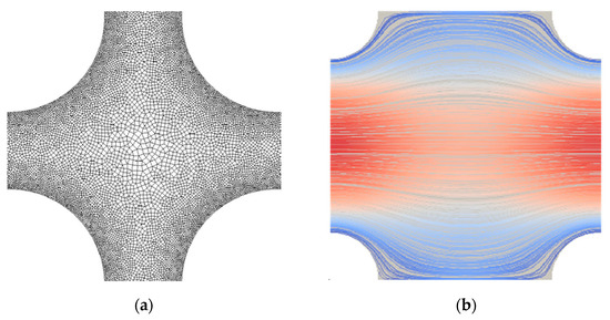
Figure 3.
Representative cases for (a) computational mesh detail between four neighboring fibers of the structure for , with mesh refinement near the fibers’ surface; (b) velocity streamlines between four fibers for , and . The color on the streamlines denotes low (blue) and high (red) velocities.
Based on the above, the constructed dataset contains four features (inputs): , , , and , as well as a target (output): . The value range of the dataset is shown in Table 1. Note that for , the negative values mean that and for the positive values mean .

Table 1.
Description and value range of the features and targets.
2.2. Data Preprocessing
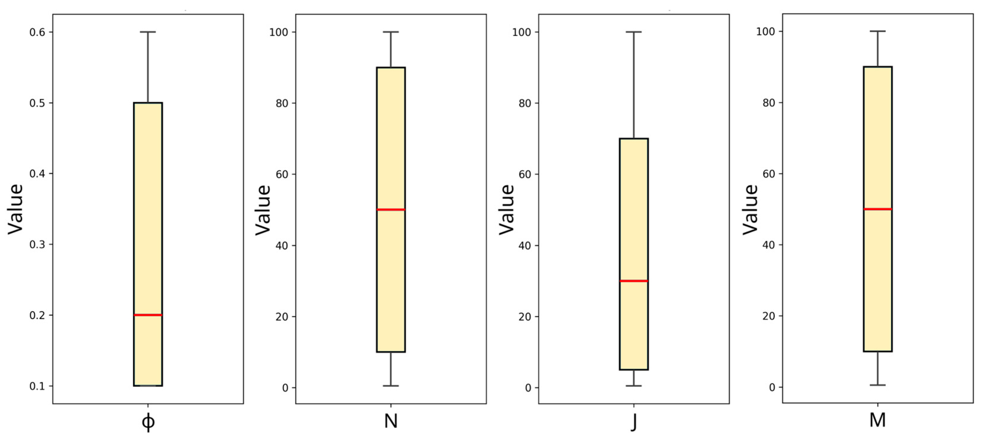
Outliers are identified as values that deviate substantially from the pattern of the dataset, leading to a reduction in the model’s accuracy and predictive power, particularly on a set of data that the ML model has never seen before. Treatment of outliers is a key preprocessing step in ML. As explained in the study by Ansari et al. [32], there are numerous approaches to detect outliers, one of which we adopt in the present study and commonly used in ML regression: the box-and-whisker plot, or simply, box-plot. With reference to Figure 4, the horizontal red line in the boxes is the median value of each feature, the box range corresponds to quartile ranges, and the whiskers symbolize the interquartile range [33]. These two ranges are calculated using the seaborn package in Python [34], customarily used for statistical data visualization. Outliers are simply values that fall outside the range of the whiskers. Based on the plot in Figure 4, there are no data points beyond the whiskers. Therefore, no outliers are detected in the dataset.
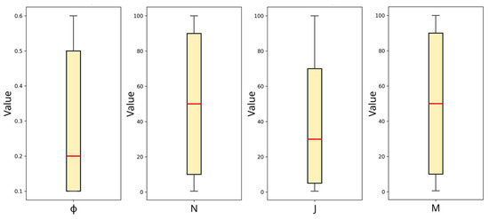
Figure 4.
Box plot for all the features for the detection of potential outliers.
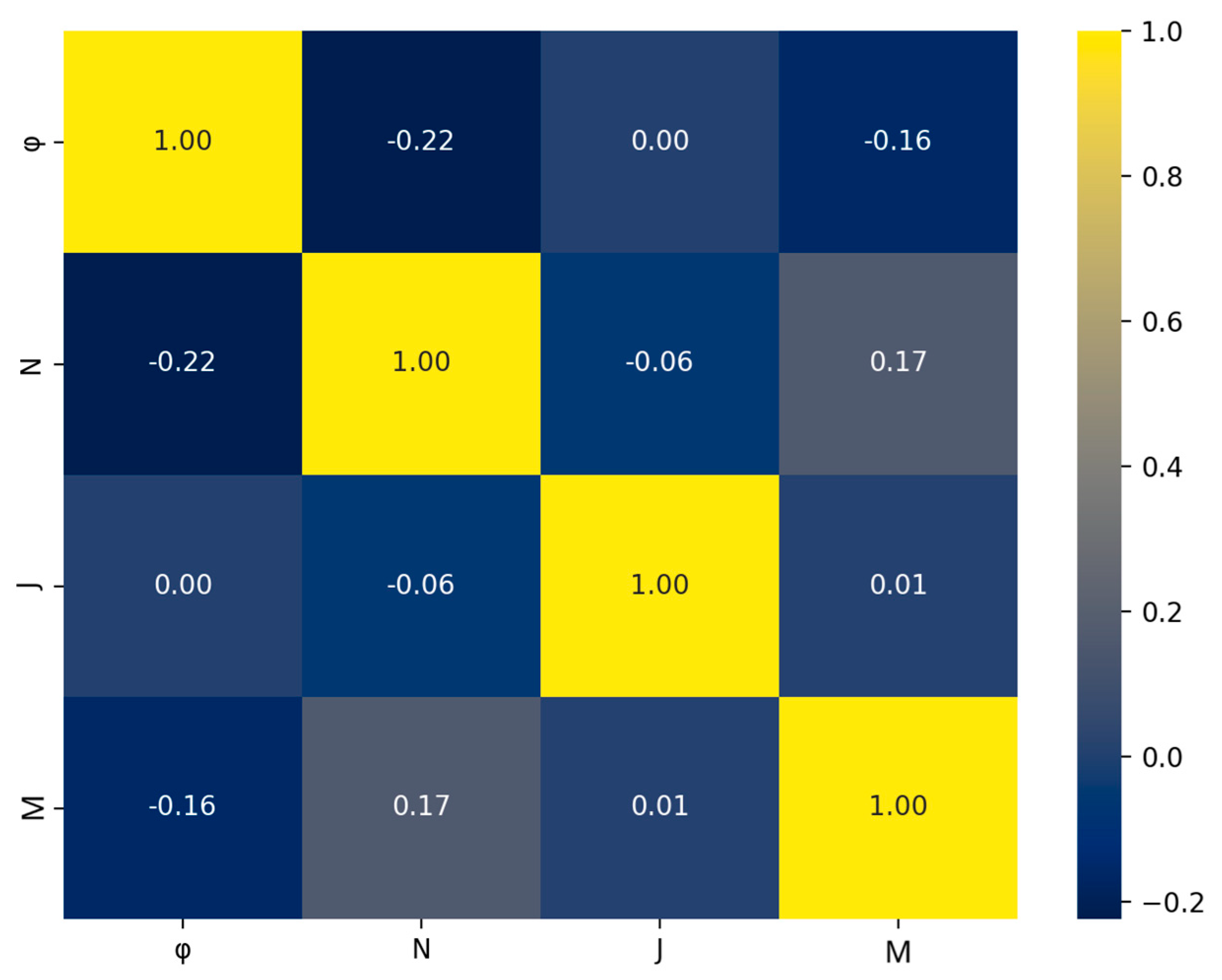
Another issue in ML models is the occurrence of multicollinearity among the features. This arises when two or more features in the dataset exhibit a high degree of correlation. Multicollinearity can lead to reduced model accuracy, a high chance of overfitting, and reduced model interpretability [35,36]. Such behavior can be effectively captured using the Spearman correlation heatmap. For the present dataset, the heatmap is shown in Figure 5. Each value in the heatmap shows how much two features from the dataset are correlated, either by exhibiting positive or negative correlation. Of course, a feature is fully correlated with itself, and this is why the diagonal cells of the heatmap show a perfect correlation, 1.00. If high correlation between two features occurs, then one of the features has to be dropped from the dataset [37,38]. A threshold value of 0.8 is frequently used as a criterion to determine the above behavior [35]; highly correlated features usually exhibit values greater than +0.8 or less than −0.8. As seen in Figure 5, the off-diagonal values range from −0.22 to +0.17, indicating weak correlation for all features of the dataset, therefore all are included.

Figure 5.
Spearman’s correlation matrix for the four features of the dataset.
Following data pre-processing, the dataset is split into two subsets of different sizes. In the primary subset, known as the training dataset, the model has access to both inputs and corresponding outputs and tries to find the underlying pattern between features and the target. The testing dataset serves as an independent set used to assess the trained model’s performance on unseen data. In the testing step, the model has access only to the features, namely the micropolar parameters , , and the solids fraction , and predicts the target, namely . This is the most crucial step for assessing the true predictive capacity of the ML model. The results of 800 numerical simulations are assigned for training the ML model, and the remaining 200 simulations are used for testing the learned model accuracy. This 80–20% data split ratio is in accordance with earlier studies [39,40].
Subsequently, feature scaling is carried out. Without scaling, features with larger numerical values may dominate the model’s learning process. This eventually leads to features with smaller ranges having a reduced impact [41,42]. Following Polychronopoulos et al. [42], features are scaled using the following equation
where denotes the scaled feature, the unscaled feature, the mean value of the feature, and the standard deviation.
2.3. Machine Learning (ML) Models and Performance
We employ six powerful ML algorithms for regression. These models are briefly explained below in Table 2. All algorithm scripts were written in the PyCharm Community Edition environment, using the scikit-learn library in Python [43]. This library contains the relevant code for DT, kNN, RF, and SVR models. The remaining models used were from the xgboost [44] and lightgbm [45] libraries.
Table 2.
Description of the ML models.
To establish the optimal set of hyperparameters for each ML model, we use the Grid Search Cross-Validation method (GridSearchCV module in scikit-learn [43]). This module systematically searches through a predefined set of parameters to find the optimal combination for an ML model and implements cross-validation (CV) to minimize overfitting. We employed a 5-fold cross-validation [41,42], where the training dataset is split into 5-folds, trained on 4-folds, and validated on the remaining 1-fold.
The trained machine learning algorithms are evaluated on the testing dataset. This is carried out using four metrics. The first one is the coefficient of determination (R2), which expresses a measure of how well the predictions approximate the results from the numerical simulations. It ranges from 1, for a perfect fit, to negative values, which typically suggests that the model predictions are very inaccurate. The coefficient is determined by
where n is the total number of samples in the dataset, the true value of the output, the predicted value of the output, and the mean value of the true output. The second performance metric is the mean squared error (MSE), given by
The third metric is the root mean squared error (RMSE), given by
The fourth performance metric is the mean absolute error (MAE), calculated from the following equation
Obviously, the lower the RMSE and MAE values, the better the predictive capacity of the ML model.
As a final step in our ML framework, we record the training time for each one of the above ML models. This is a crucial factor that must be taken into consideration, particularly when considering scalability, i.e., the ML model’s ability to handle increasing amounts of data without sacrificing its predictive performance. Therefore, when selecting an ML algorithm, it is absolutely necessary to balance the predictive capacity of the model with the training time. The training time is defined as
where is the time when training begins, and when it ends.
2.4. Model Interpretability
ML models are frequently referred to as black boxes, since the algorithm’s internal structure is too complicated for a human being to understand and ultimately grasp how the algorithm makes its predictions. In several fields of medicine and engineering, where ML is already applied, interpretability techniques are used to help explain individual predictions or global behavior of the ML model, which reveals the “why” behind decisions.
In the present study, to interpret the predictions of the best-performing ML model, we use Shapley Additive exPlanations (SHAP) values analysis, a technique that belongs to the broader field of eXplainable artificial intelligence (XAI) [46]. SHAP analysis aims at explaining a prediction by computing the contribution of each feature to that prediction. The SHAP analysis framework has its origins in cooperative game theory, and the contribution of each feature is represented by the so-called Shapley value [47]. In general, exact computation of the Shapley values is a challenging task and, more importantly, the computational burden is extremely high due to multiple possibilities of the feature subset space [48]. Therefore, different SHAP variants have been proposed to calculate the Shapley values, including KernelSHAP and TreeSHAP, for specific ML algorithms [49]. For example, XGBoost, Decision Trees, and Random Forest regression models, which are tree-based models, naturally match to TreeSHAP.
3. Results
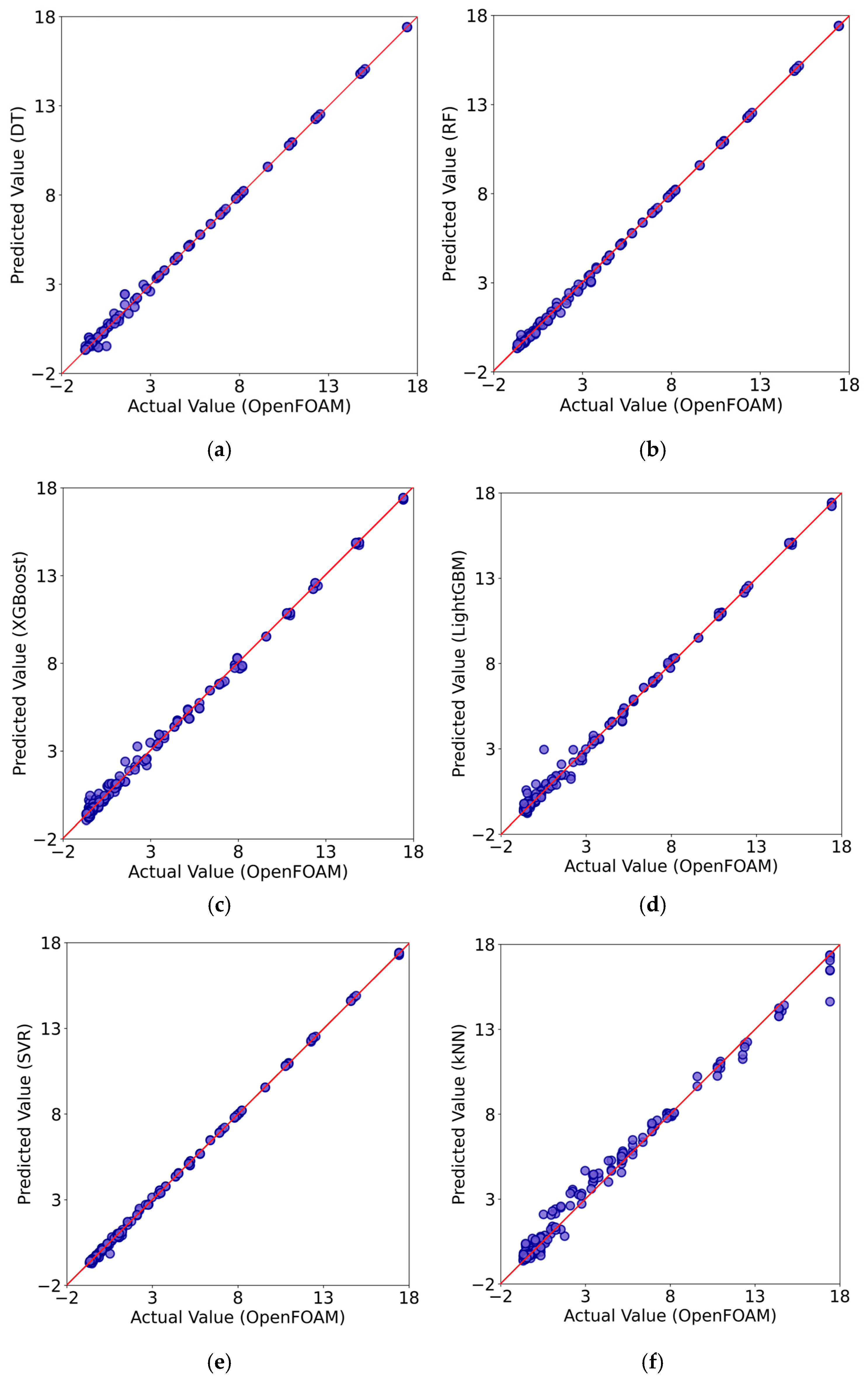
Figure 6 compares the predictions of each ML algorithm used with the ones obtained from OpenFOAM numerical simulations for the testing dataset. As explained earlier, the testing dataset is particularly important because the trained model makes new predictions on data that was not included in the learning process and essentially reveals the true predictive power of the ML model. The red diagonal line in Figure 6 represents the scenario for perfect predictions for each instance. The further the data points are from this line, the larger the associated errors. Such plots provide a quick visual assessment of the ML model performance on new data instances and the capacity of the algorithm to generalize. Overall, the data points align very well along the diagonal line for most models, indicating strong predictive accuracy. However, there are some evident deviations in the predictions for the cases of kNN and LightGBM, especially in the lower range of the values, suggesting a relatively reduced performance of the models in generalization. From a general viewpoint, all six ML models behave reasonably well, but close inspection of the data point distribution around the diagonal reveals that the Random Forest and SVM algorithms may behave better in predictions than the rest.
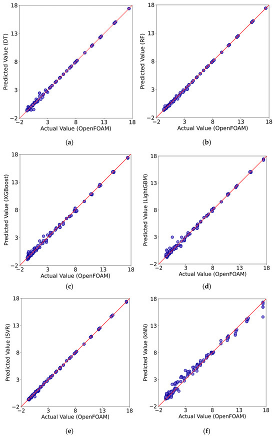
Figure 6.
Comparison of the results for the testing dataset from the numerical simulations using the OpenFOAM software and the predictions by Decision Trees (DT) (a); Random Forest (RF) (b); XGBoost (c); LightGBM (d); Support Vector Regression (SVR) (e); k-Nearest Neighbors (kNN) (f) ML models.
A more precise quantification for the above can be provided by calculating the values and the relevant error values for each one of the ML models. This is illustrated in Table 3. The lowest predictions, compared with the rest, come from the kNN and LightGBM algorithms with and , respectively. In contrast, the top-performing algorithms are Random Forest (RF) and Support Vector Regression (SVR), where in both cases values are almost close to unity (for RF: and for SVR: ). However, RF exhibits lower errors than SVR.
Table 3.
and error metrics of all the machine learning (ML) models.
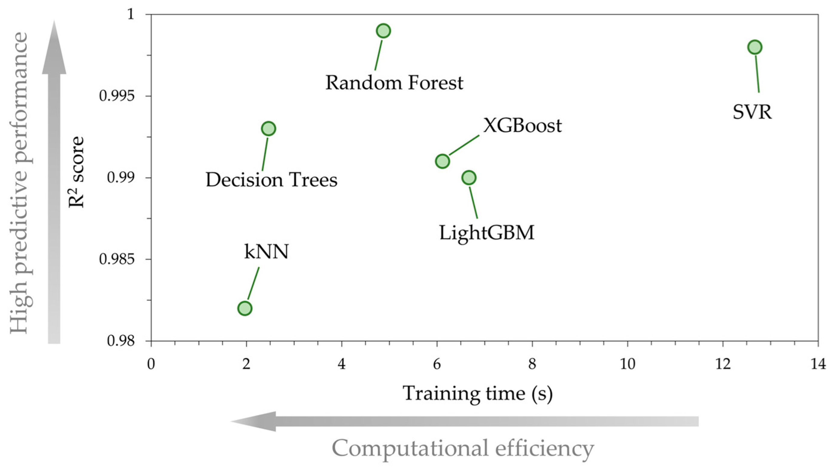
Figure 7 is a plot that illustrates a comparative analysis of the ML models, where the predictive accuracy of each ML model, quantified by , is compared against the computational efficiency, quantified by the training time. DT and kNN models achieved the lowest training times, of the order of 2 s, which is reasonable since both models have a relatively simple internal architecture. For example, in DT regression the model is built based on only one tree, whereas an ensemble mode of multiple trees is used in models such as RF or gradient boosting. This is why for the latter models in the present study, the training time ranges between 5 s and 7 s. Yet, the RF algorithm, although it requires more time to train the data as compared to DT and kNN, achieves a much better prediction accuracy than XGBoost and LightGBM. The SVR model, has a nearly identical predictive performance to RF, but to achieve this high accuracy, more training time is required, approximately 13 s, which is considerably higher than RF. Based on the above, the RF model achieves a reasonable balance between high accuracy and low training time compared with the other models. Therefore, for the subsequent SHAP analysis, we use the RF model.

Figure 7.
Comparative analysis of the ML models’ predictive performance () and computational efficiency (training time in seconds). The best ML model scalability is achieved when high accuracy is combined with low computational cost.
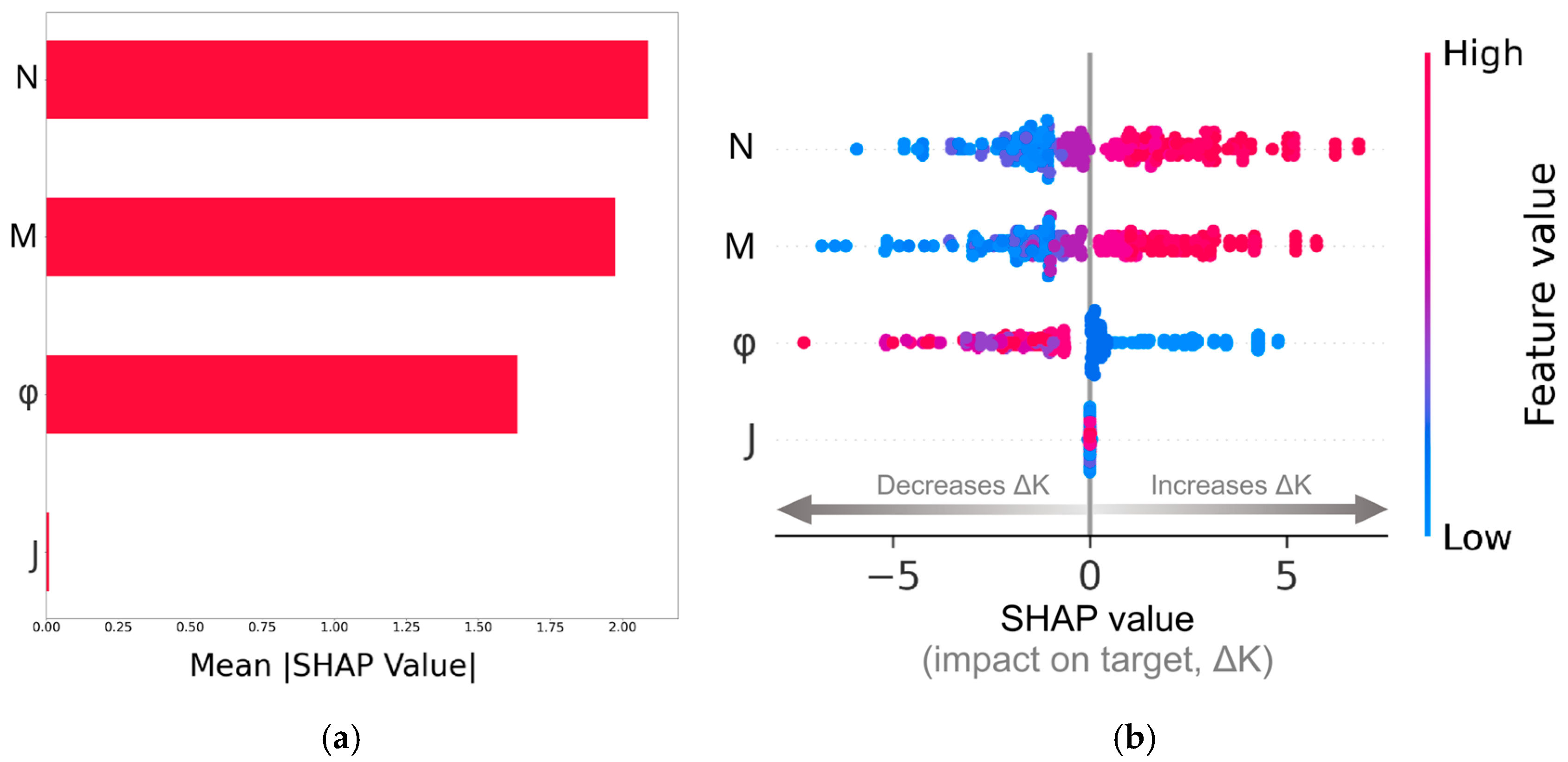
The SHAP analysis of the results using the Random Forest (RF) algorithm is shown in Figure 8. We have followed Molnar [49] and selected the testing-dataset points for the analysis. Figure 8a is a horizontal bar chart displaying the mean absolute SHAP values for each feature. This plot quantifies the contribution of each feature to the model’s prediction of . From the feature ranking shown in Figure 8a, it is evident that the dimensionless spin-gradient viscosity and the dimensionless vortex viscosity have the highest contributions to the predictions made by the RF model. The solid volume fraction of the porous structure is ranked in the third position with a mean absolute SHAP value lower than those of the and micropolar fluid properties, suggesting that the porous microstructure has a secondary impact on the flow dynamics. The dimensionless micro-inertia has a negligible impact on the predictions. This is somewhat expected, since we have assumed in the analysis that . Nonetheless, the fact that the RF algorithm also predicts that this feature does not contribute to the model decisions, makes the algorithm robust, especially if we take into account the fact that it refers to the testing dataset, where the model was agnostic to the target.
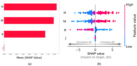
Figure 8.
Feature importance ranking using the mean absolute SHAP value (a); SHAP summary plot (b).
More information on the decisions made by the RF model can be deduced from the plot shown in Figure 8b, frequently referred to in the ML literature as the SHAP summary plot. It shows the SHAP values distribution for each feature, revealing the directional feature influence on the target, . The horizontal x-axis in the plot corresponds to the SHAP values, and the vertical y-axis ranks the features in descending order of importance. Each data point in the plot corresponds to a specific sample within the dataset. The color bar to the right of the plot represents the magnitude of the features, with blue color for low feature values and red color for high feature values. The horizontal placement of each data point exhibits the impact of the feature on the model’s prediction values. This indicates whether a higher or lower feature value leads to a higher prediction value (positive SHAP values) or a lower prediction value (negative SHAP values). By higher prediction values we mean higher values, i.e., the permeability of the micropolar fluid is higher than the Newtonian fluid. A key observation from this plot is that high values of and are predominantly associated with positive SHAP values, meaning that increasing these parameters generally increases the difference between the hydraulic permeability of the micropolar fluid and the Newtonian fluid (increasing the target values). Therefore, enhancing spin-gradient viscosity promotes flow, potentially by facilitating rotational fluid motion that reduces resistance in the confined fluid space between the fibers. This is also the case for the feature, as vortex viscosity plays a crucial role in modifying shear stresses and momentum transport in micropolar fluids. In sharp contrast, the solid volume fraction exhibits a different behavior. Increasing leads to SHAP values that are generally negative, which means that decreases, suggesting that the effective permeability of the structure with a micropolar fluid becomes comparable to that of a Newtonian fluid. This behavior aligns with the physical flow setting in the following way. At low solid fractions, the increased surface area for micropolar fluid–solid interaction might amplify the effects of rotational viscosity, revealing a micropolar-dominant regime. On the other hand, at higher solid fractions, the open space between the fibers is reduced, and this increased blockage and tortuosity lead to a viscous-dominant regime. In this flow regime, the negative SHAP values suggest that the permeability of the micropolar fluid tends to be similar to that of the Newtonian fluid.
4. Discussion and Conclusions
In the current study, we have presented an ML framework to predict the permeability of a micropolar fluid flowing in a porous structure. Traditional theoretical models have provided valuable insights into fluid flow through fibrous media [19,20,22], but they often rely on the simplifying assumption of a Newtonian fluid. The present ML framework offers a complementary approach by directly learning the complex relationship between micropolar fluid properties, structural parameters, and hydraulic permeability from numerical simulation data. This data-driven approach captures the complex interactions of the bio-fluid with the surrounding fibers, which may be overlooked by traditional models, particularly in cases where micropolar effects are significant. A dataset of 1000 samples was obtained by carrying out numerical simulations in the OpenFOAM software. Ideally, we would require a large dataset, such as, for instance, the dataset by Wong et al. [50] containing half a billion data points associated with insulin transcription in human pancreatic islet cells. However, there is nothing remotely equivalent for fibrous biomaterials with micropolar fluids. Data generation using numerical simulations is customarily carried out if experimental data are not available. In fact, data generated from computational fluid dynamics packages (CFD) have been used to train ML models for rupture status assessments of intracranial aneurysms [51] and blood flow with red cell distribution in capillary vessel networks [52]. Moreover, in the present study, the porous structure was assumed to be represented by an idealized geometry of nine parallel fibers in a square periodic mode. We have built this foundational model to isolate the impact of micropolar fluid properties. A hexagonal array of cylinders could be further employed. It should be pointed out that the fibers in biomaterials may often exhibit more complex and disordered microstructures, such as random fiber orientations and fiber diameter variations, as, for example, in healthy and injured collagen tissues [24]. These effects can be easily embedded into the current ML framework by increasing the number of features. For example, in disordered fibrous media, the mean minimum interfiber spacing [23,53] can be included as one additional feature. Therefore, the present dataset can be enriched and then be used to build more sophisticated ML models, within the present framework, capable of predicting hydraulic permeability in more realistic settings. This is a significant future direction.
The dimensionless form of the flow equations allowed us to use physically-informed features related to the micropolar fluid and porous structure: dimensionless spin-gradient viscosity; dimensionless vortex viscosity; dimensionless microinertia; solid volume fraction. Dimensionless groups tend to require less data for good algorithm performance compared to raw input data. Combined with feature outlier detection and checking for multicollinearity, we employed six powerful ML regression algorithms to predict the permeability of the assumed porous structure, expressed as the difference between the permeability of a micropolar fluid and that of a Newtonian one. The ML algorithms generally showed a high accuracy and reasonably low prediction errors. Random Forest (RF) achieved the best balance between accuracy of the predictions and training time. Specifically, it achieved ; MAE = 0.0412; MSE = 0.0132; and RMSE = 0.1152 with a training time of only 5 s. It should be noted that a numerical simulation to calculate the permeability of a micropolar fluid with features (inputs) belonging to the testing dataset ranged from 30 to 40 min, which is substantially higher than the RF training time. Therefore, the RF algorithm may be an ideal candidate for fully 3D micropolar fluid flow in anisotropic physiological porous structures consisting of fully 3D disoriented and misaligned fibers, where the computational time is expected to increase.
As explained earlier, ML algorithms are frequently characterized by a black-box nature. To overcome this limitation and enhance the transparency of our ML framework, we employed SHAP analysis, which is part of a larger field often termed as eXplainable artificial intelligence (XAI). The SHAP analysis revealed that the dimensionless spin-gradient viscosity and dimensionless vortex viscosity are the two dominant players in the decisions made by RF. Specifically, SHAP analysis showed that higher values of N and M result in higher permeability of a micropolar fluid than its Newtonian counterpart. This may be associated with the combined effect of velocity increase that enhances the bulk flow and the reduced shear stress near the fiber wall, caused by the increased rotational interactions of the fluid microelements. This observation aligns well with the increase of bulk flow of a micropolar fluid, describing blood, in a human carotid model [9]. The SHAP analysis further demonstrated that the effect of the solid volume fraction in the structure is secondary, compared to the micropolar fluid properties. At low , the flow is micropolar-dominant, leading to a higher permeability of the micropolar fluid than the Newtonian, while in high , the flow enters a viscous-dominated regime and the difference in permeability between a micropolar and a Newtonian fluid is reduced. The micro-inertia feature was correctly predicted by the SHAP analysis as having no contribution to the permeability prediction, since the flow is assumed to have . The above results are significant from both a theoretical fluid mechanics perspective and a biomedical engineering standpoint. For example, in collagen tissues, promoting higher permeability means improved mass transport, which is crucial for nutrient delivery, waste removal, as well as overall tissue health [54]. Since micropolar effects can enhance permeability, introducing microstructural agents (e.g., rod-like molecules) may tune the rotational viscosities and promote flow. In synovial fluid, for example, there are suspended hyaluronic acid chains and globule proteins [55], and understanding how and affect the flow in the porous cartilage of fibrous extracellular matrix may lead to more accurate models, and perhaps therapeutic strategies. Moreover, in cardiovascular tissue engineering, efficient nutrient and oxygen transport is significant for the survival and function of engineered tissues [56]. The SHAP analysis suggests that tailoring the properties of the micropolar bio-fluid and the porosity of the structure could be a significant direction to enhance mass transport within the fabricated structure. This is equally important in bone tissue engineering, where efficient nutrient delivery and cell adhesion are required, balanced by optimal porosity (or solid volume fraction) for sufficient mechanical integrity of the structure under various mechanical loadings [57]. Furthermore, in electrospun microfiber mats with applications in bio-filtration and stimulation of biological cells, the adjacent fibers may undergo viscous sintering (coalescence) [58] upon applying an electrochemical stimulus and produce different pore sizes [59]. Consequently, in these biomaterials, the solid volume fraction and the interaction of the transported biofluids are critical factors, and the SHAP analysis may contribute to tailored designs.
In conclusion, the present ML framework provides a robust tool for determining the permeability in fibrous biomaterials. The framework has not only the capacity to make fast and reliable permeability predictions, but also gives a fundamental understanding of the effect of the involved process parameters on a physical basis via SHAP analysis. Therefore, the proposed ML framework may lay the foundations for designing fine-tuned fluids or fibrous biomaterials with enhanced permeability, which could potentially lead to better functionality. Ultimately, future research should focus on conducting controlled experiments to measure the hydraulic permeability in such systems with well-characterized microstructures using micropolar fluids with known properties. The experimental results would serve as a significant benchmark for our ML framework and for further model refining.
Author Contributions
Conceptualization, N.D.P. and E.K.; methodology, N.D.P.; software, N.D.P., E.K. and A.T.; validation, N.D.P. and A.T.; formal analysis, N.D.P.; investigation, N.D.P. and E.K.; writing—original draft preparation, N.D.P.; writing—review and editing, N.D.P., E.K. and T.D.P.; supervision, T.D.P. All authors have read and agreed to the published version of the manuscript.
Funding
This research received no external funding.
Data Availability Statement
The original contributions presented in this study are included in the article. Further inquiries can be directed to the corresponding authors.
Conflicts of Interest
The authors declare no conflicts of interest.
Abbreviations
The following abbreviations are used in this manuscript:
| AI | Artificial Intelligence |
| CFD | Computational Fluid Dynamics |
| CV | Cross Validation |
| DT | Decision Trees |
| kNN | k-Nearest Neighbors |
| LightGBM | Light Gradient-Boosting Machine |
| MAE | Mean Absolute Error |
| ML | Machine learning |
| MSE | Mean Squared Error |
| OpenFOAM | Open Field Operation And Manipulation |
| PHAs | Polyhydroxyalkanoates |
| PLAs | Polylactides |
| RF | Random Forest |
| RMSE | Root Mean Squared Error |
| SHAP | Shapley Additive exPlanations |
| SVR | Support Vector Regression |
| XAI | eXplainable Artificial Intelligence |
| XGBoost | eXtreme Gradient Boosting |
References
- Mamidi, N.; García, R.G.; Martínez, J.D.H.; Briones, C.M.; Ramos, A.M.M.; Tamez, M.F.L.; Del Valle, B.G.; Segura, F.J.M. Recent Advances in Designing Fibrous Biomaterials for the Domain of Biomedical, Clinical, and Environmental Applications. ACS Biomater. Sci. Eng. 2022, 8, 3690–3716. [Google Scholar] [CrossRef]
- Ma, L.; Dong, W.; Lai, E.; Wang, J. Silk fibroin-based scaffolds for tissue engineering. Front. Bioeng. Biotechnol. 2024, 12, 1381838. [Google Scholar] [CrossRef]
- Gough, C.R.; Callaway, K.; Spencer, E.; Leisy, K.; Jiang, G.; Yang, S.; Hu, X. Biopolymer-based filtration materials. ACS Omega 2021, 6, 11804–11812. [Google Scholar] [CrossRef] [PubMed]
- Azimi, B.; Maleki, H.; Zavagna, L.; De la Ossa, J.G.; Linari, S.; Lazzeri, A.; Danti, S. Bio-based electrospun fibers for wound healing. J. Funct. Biomater. 2020, 11, 67. [Google Scholar] [CrossRef]
- Celikkin, N.; Rinoldi, C.; Constantini, M.; Trombetta, M.; Rainer, A.; Święszkowski, W. Naturally derived proteins and glycosaminoglycan scaffolds for tissue engineering applications. Mater. Sci. Eng. C 2017, 78, 1277–1299. [Google Scholar] [CrossRef]
- Hamerman, D.; Rosenberg, L.C.; Schubert, M. Diarthrodial joints revisited. J. Bone Jt. Surg. 1970, 52, 725. [Google Scholar] [CrossRef]
- Hernandez, J.L.; Woodrow, K.A. Medical applications of porous biomaterials: Features of porosity and tissue-specific implications for biocompatibility. Adv. Healthc. Mater. 2022, 11, 2102087. [Google Scholar] [CrossRef]
- Babitha, S.; Rachita, L.; Karthikeyan, K.; Shoba, E.; Janani, I.; Poornima, B.; Sai, K.P. Electrospun protein nanofibers in healthcare: A review. Int. J. Pharm. 2017, 523, 52–90. [Google Scholar] [CrossRef]
- Karvelas, E.; Sofiadis, G.; Papathanasiou, T.; Sarris, I. Effect of micropolar fluid properties on the blood flow in a human carotid model. Fluids 2020, 5, 125. [Google Scholar] [CrossRef]
- Tandon, P.N.; Jaggi, S. A polar model for synovial fluid with reference to human joints. Int. J. Mech. Sci. 1979, 21, 161–169. [Google Scholar] [CrossRef]
- Benos, L.; Ninos, G.; Polychronopoulos, N.D.; Exomanidou, M.-A.; Sarris, I. Natural convection of blood-magnetic iron oxide bio-nanofluid in the context of hyperthermia treatment. Computation 2022, 10, 190. [Google Scholar] [CrossRef]
- Eringen, A.C. Theory of micropolar fluids. J. Math. Mech. 1966, 16, 1–18. [Google Scholar] [CrossRef]
- Aslani, K.-E.; Benos, L.; Tzirtzilakis, E.; Sarris, I.E. Micromagnetorotation of MHD micropolar flows. Symmetry 2020, 12, 148. [Google Scholar] [CrossRef]
- Aslani, K.-E.; Tzirtzilakis, E.; Sarris, I.E. On the mechanics of conducting micropolar fluids with magnetic particles: Vorticity-microrotation difference. Phys. Fluids 2024, 36, 102006. [Google Scholar] [CrossRef]
- Ferland, P.; Guittard, D.; Trochu, F. Concurrent methods for permeability measurement in resin transfer molding. Polym. Compos. 1996, 17, 149–158. [Google Scholar] [CrossRef]
- Parnas, R.S.; Flynn, K.M.; Dal-Favero, M.E. A permeability database for composites manufacturing. Polym. Compos. 1997, 18, 623–633. [Google Scholar] [CrossRef]
- Gebart, B.R.; Lidström, P. Measurement of in-plane permeability of anisotropic fiber reinforcements. Polym. Compos. 1996, 17, 43–51. [Google Scholar] [CrossRef]
- Happel, J. Viscous flow relative to arrays of cylinders. AIChE J. 1959, 5, 174–177. [Google Scholar] [CrossRef]
- Gebart, B.R. Permeability of unidirectional reinforcements for RTM. J. Compos. Mater. 1992, 26, 1100–1133. [Google Scholar] [CrossRef]
- Tamayol, A.; Bahrami, M. Analytical determination of viscous permeability of fibrous porous media. Int. J. Heat. Mass. Transf. 2009, 52, 2407–2414. [Google Scholar] [CrossRef]
- Papathanasiou, T.D. A structure-oriented micro mechanical model for viscous flow through square arrays of fibre clusters. Compos. Sci. Technol. 1996, 56, 1055–1069. [Google Scholar] [CrossRef]
- Chen, X.; Papathanasiou, T.D. On the variability of the Kozeny constant for saturated flow across unidirectional disordered fiber arrays. Compos. Part A Appl. Sci. Manuf. 2006, 37, 836–846. [Google Scholar] [CrossRef]
- Chen, X.; Papathanasiou, T.D. The transverse permeability of disordered fiber arrays: A statistical correlation in terms of the mean nearest interfiber spacing. Transp. Porous Media 2008, 71, 233–351. [Google Scholar] [CrossRef]
- Erisken, C.; Tsiantis, A.; Papathanasiou, T.D.; Karvelas, E.G. Collagen fibril diameter distribution affects permeability of ligament tissue: A computational study on healthy and injured tissues. Comput. Methods Programs Biomed. 2020, 196, 105554. [Google Scholar] [CrossRef]
- Karvelas, E.G.; Tsiantis, A.; Papathanasiou, T.D. Effect of micropolar fluid properties on the hydraulic permeability of fibrous biomaterials. Comput. Methods Programs Biomed. 2020, 185, 105135. [Google Scholar] [CrossRef]
- Zade, A.; Neogi, S.; Kuppusamy, R.R.P. Effect of process and material parameters on the permeabilities of reinforcement mats: Experimentations and machine learning techniques. Fibers Polym. 2024, 25, 2285–2302. [Google Scholar] [CrossRef]
- Caglar, B.; Broggi, G.; Ali, M.A.; Orgéas, L.; Michaud, V. Deep learning accelerated prediction of the permeability of fibrous microstructures. Compos. Part A Appl. Sci. Manuf. 2022, 158, 106973. [Google Scholar] [CrossRef]
- Froning, D.; Hoppe, E.; Peters, R. The applicability of machine learning methods to the characterization of fibrous gas diffusion layers. Appl. Sci. 2023, 13, 6981. [Google Scholar] [CrossRef]
- Schmidt, T.; Natarajan, D.K.; Duhovic, M.; Cassola, S.; Nuske, M.; May, D. Numerical data generation for building machine learning models for permeability estimation of fibrous structures. Polym. Compos. 2025. [Google Scholar] [CrossRef]
- Sarifuddin; Chakravarty, S.; Mandal, P.K. Heat transfer to micropolar fluid flowing through an irregular arterial constriction. Int. J. Heat Mass Transf. 2013, 56, 538–551. [Google Scholar] [CrossRef]
- Weller, H.; Tabor, G.; Jasak, H.; Fureby, C. A tensorial approach to computational continuum mechanics using object-oriented techniques. Comput. Phys. 2010, 12, 620–631. [Google Scholar] [CrossRef]
- Ansari, S.; Nassif, A.B.; Mahmoud, S.; Majzoub, S.; Almajali, E.; Jarndal, A.; Bonny, T.; Alnajjar, K.A.; Hussain, A. Impact of outliers on regression and classification models: An empirical analysis. In Proceedings of the International Conference Developments in eSystems Engineering (DeSE), Khorfakkan, United Arab Emirates, 6–8 November 2024. [Google Scholar]
- Mazarei, A.; Sousa, R.; Mendes-Moreira, J.; Molchanov, S.; Ferreira, H.M. Online boxplot derived outlier detection. Int. J. Data Sci. Anal. 2025, 19, 83–97. [Google Scholar] [CrossRef]
- Seaborn: Statistical Data Visualization. Available online: https://seaborn.pydata.org/ (accessed on 15 March 2025).
- Ali, T.; Onyelowe, K.C.; Mahmood, M.S.; Qureshi, M.Z.; Kahla, N.B.; Rezzoug, A.; Deifalla, A. Advanced and hybrid machine learning techniques for predicting compressive strength in palm oil fuel ash-modified concrete with SHAP analysis. Sci. Rep. 2025, 15, 4997. [Google Scholar] [CrossRef] [PubMed]
- Drobnič, F.; Kos, A.; Pustišek, M. On the interpretability of machine learning models and experimental feature selection in case of multicollinear data. Electronics 2020, 9, 761. [Google Scholar] [CrossRef]
- Karakasidis, T.E.; Sofos, F.; Tsonos, C. The electrical conductivity of ionic liquids: Numerical and analytical machine learning approaches. Fluids 2022, 7, 321. [Google Scholar] [CrossRef]
- Sofos, F.; Papakonstantinou, C.G.; Valasaki, M.; Karakasidis, T.E. Fiber-reinforced polymer confined concrete: Data-driven predictions of compressive strength utilizing machine learning techniques. Appl. Sci. 2023, 13, 567. [Google Scholar] [CrossRef]
- Kumar, A.; Arora, H.C.; Kappor, N.R.; Mohammed, M.A.; Kumar, K.; Majumdar, A.; Thinnukool, O. Compressive strength prediction of lightweight concrete: Machine learning models. Sustainability 2022, 14, 2404. [Google Scholar] [CrossRef]
- Hemdan, E.E.-D.; Alshathri, S.; Elwahsh, H.; Ghoneim, O.A.; Sayed, A. MAL-XSEL: Enhancing industrial web malware detection with an explainable stacking ensemble model. Processes 2025, 13, 1329. [Google Scholar] [CrossRef]
- Polychronopoulos, N.D.; Moustris, K.; Karakasidis, T.; Sikora, J.; Krasinskyi, V.; Sarris, I.E.; Vlachopoulos, J. Machine learning for screw design in single-screw extrusion. Polym. Eng. Sci. 2025, 65, 2607–2623. [Google Scholar] [CrossRef]
- Polychronopoulos, N.D.; Sarris, I.; Vlachopoulos, J. Implementation of machine learning in flat die extrusion of polymers. Molecules 2025, 30, 1879. [Google Scholar] [CrossRef]
- Pedregosa, F.; Varoquaux, G.; Gramfort, A.; Michel, V.; Thirion, B.; Grisel, O.; Blondel, M.; Prettenhofer, P.; Weiss, R.; Dubourg, V.; et al. Scikit-learn:machine learning in Python. J. Mach. Learn. Res. 2011, 12, 2825–2830. [Google Scholar]
- DMLC XGBoost Scalable and Flexible Gradient Boosting. Available online: https://xgboost.ai/ (accessed on 18 March 2025).
- LightGBM. Available online: https://lightgbm.readthedocs.io/en/stable/ (accessed on 18 March 2025).
- Antoniadi, A.M.; Du, Y.; Guendouz, Y.; Wei, L.; Mazo, C.; Becker, B.A.; Mooney, C. Current challenges and future opportunities for XAI in machine learning-based clinical decision support systems: A systematic review. Appl. Sci. 2021, 11, 5088. [Google Scholar] [CrossRef]
- Štrumbelj, E.; Kononenko, I. An efficient explanation of individual classifications using game theory. J. Mach. Learn. Res. 2010, 11, 1–18. [Google Scholar]
- Feng, D.-C.; Wang, W.-J.; Mangalathu, S.; Taciroglu, E. Interpretable XGBoost-SHAP machine-learning model for shear strength prediction of squat RC walls. J. Struct. Eng. 2021, 147, 04021173. [Google Scholar] [CrossRef]
- Molnar, C. Interpretable Machine Learning. 2020. Available online: https://christophm.github.io/interpretable-ml-book/ (accessed on 12 April 2025).
- Wong, W.K.M.; Thorat, V.; Joglekar, M.V.; Dong, C.X.; Lee, H.; Chew, Y.V.; Bhave, A.; Hawthorne, W.J.; Engin, F.; Pant, A.; et al. Analysis of half a billion datapoints across ten machine-learning algorithms identifies key elements associated with insulin transcription in human pancreatic islet cells. Front. Endocrinol. 2022, 13, 853863. [Google Scholar] [CrossRef] [PubMed]
- Mu, N.; Rezaeitaleshmahalleh, M.; Lyu, Z.; Wang, M.; Tang, J.; Strother, C.M.; Gemmete, J.J.; Pandey, A.S.; Jiang, J. Can we explain machine learning-based prediction for rupture status assessments of intracranial aneurysms? Biomed. Phys. Eng. Express 2023, 9, 037001. [Google Scholar] [CrossRef]
- Ebrahimi, S.; Bagchi, P. Application of machine learning in predicting blood flow and red cell distribution in capillary vessel networks. J. R. Soc. Interface 2022, 19, 20220306. [Google Scholar] [CrossRef] [PubMed]
- Yazdchi, K.; Srivastava, S.; Luding, S. Micro-macro relations for flow through random arrays of cylinders. Compos. Part A Appl. Sci. Manuf. 2012, 43, 2007–2020. [Google Scholar] [CrossRef]
- Antoine, E.E.; Vlachos, P.P.; Rylander, M.N. Review of collagen I hydrogels for bioengineered tissue microenvironments: Characterization of mechanics, structures and transport. Tissue Eng. Part B Rev. 2014, 20, 683–696. [Google Scholar] [CrossRef]
- Seekell III, R.P.; Dever, R.; Zhu, Y. Control hydrogel-hyaluronic acid aggregation toward the design of biomimetic superlubricants. Biomacromolecules 2014, 15, 2760–2768. [Google Scholar] [CrossRef]
- Rademakers, T.; Horvath, J.M.; van Blitterswijk, C.A.; LaPointe, V.L.S. Oxygen and nutrient delivery in tissue engineering: Approaches to graft vascularization. J. Tissue Eng. Regen. Med. 2019, 13, 1815–1829. [Google Scholar] [CrossRef] [PubMed]
- Ma, Q.; Miri, Z.; Haugen, H.J.; Moghanian, A.; Loca, D. Significance of mechanical loading in bone fracture healing, bone regeneration, and vascularization. J. Tissue Eng. 2023, 14, 20417314231172573. [Google Scholar] [CrossRef] [PubMed]
- Polychronopoulos, N.D.; Sarris, I.E.; Vlachopoulos, J. A viscous sintering model for pore shrinkage in packing of cylinders. Rheol. Acta 2021, 60, 397–408. [Google Scholar] [CrossRef]
- Kerr-Phillips, T.E.; Woehling, V.; Agniel, R.; Nguyen, G.T.M.; Vidal, F.; Kilmartin, P.; Plesse, C.; Travas-Sejdic, J. Electrospun rubber fibre mats with electrochemically controllable pore sizes. J. Mater. Chem. B 2015, 3, 4249. [Google Scholar] [CrossRef]


Disclaimer/Publisher’s Note: The statements, opinions and data contained in all publications are solely those of the individual author(s) and contributor(s) and not of MDPI and/or the editor(s). MDPI and/or the editor(s) disclaim responsibility for any injury to people or property resulting from any ideas, methods, instructions or products referred to in the content. |
© 2025 by the authors. Licensee MDPI, Basel, Switzerland. This article is an open access article distributed under the terms and conditions of the Creative Commons Attribution (CC BY) license (https://creativecommons.org/licenses/by/4.0/).