Abstract
The vector-based method is a technique that analyzes and processes data by vectoring them. It represents data points as multidimensional vectors that can be calculated and compared in a high-dimensional space. This method has significant advantages in prediction, mainly in the ability to process high-dimensional data, the effect of capturing nonlinear relationships, and the high efficiency on large datasets. First, the vector-based method effectively handles high-dimensional data, is not limited by the data dimension, and is suitable for complex multivariate analysis. Second, it is able to capture the nonlinear relationships between the data and identify potential patterns and trends through computation and comparisons in a high-dimensional space. Finally, the high efficiency of vector-based methods on large datasets enables it to quickly process and analyze large amounts of data and improve the accuracy and reliability of prediction. These characteristics make the vector-based method particularly applicable in mine pressure appearance prediction, which can more accurately analyze ore pressure data, identify potential risks, and then improve the level of mine safety management.
1. Introduction
The prediction of mine pressure behavior in working faces is a critical challenge in coal mining safety, particularly as mining depths increase and geological conditions become more complex [1,2]. Traditional methods for mine pressure prediction, such as empirical formulas and linear regression models, often struggle to handle high-dimensional monitoring data and capture the nonlinear relationships inherent in mine pressure dynamics [3]. These limitations have driven the need for more advanced data-driven approaches that can effectively process multi-source information and improve prediction accuracy.
The vector-based method, a technique that transforms data into multidimensional vectors for analysis in high-dimensional spaces, offers significant advantages in addressing these challenges [4,5]. By converting raw data into vectors, this method enables efficient processing of high-dimensional datasets, captures complex nonlinear patterns through geometric operations (e.g., vector distances and angles), and maintains computational efficiency even with large-scale data. These characteristics make it particularly suitable for mine pressure prediction, where multiple influencing factors (e.g., roof subsidence, mining progress, and seam thickness) interact in nonlinear ways [5,6,7].
Existing studies on mine pressure prediction have increasingly adopted machine learning algorithms like support vector machines (SVM) and neural networks [1,3,4,5,6,7,8]. However, these approaches often rely on empirical feature engineering, suffer from dimensionality reduction issues, or require extensive computational resources. The vector-based method addresses these gaps by providing a systematic framework for data preprocessing, feature selection, and model training. For instance, data preprocessing steps such as noise filtering, missing value imputation (using mean/median methods), and outlier detection (via Z-score or boxplot techniques) ensure high-quality input data. Feature selection employs filter methods (e.g., variance thresholding, correlation analysis) and embedded methods (e.g., principal component analysis, PCA) to reduce dimensionality while retaining critical information [9,10,11,12].
In this study, a vector-based prediction model was developed and validated through a four-step process: data preprocessing, feature selection, model training, and validation. Three models were compared: multiple linear regression, SVM with a radial basis function (RBF) kernel, and a multi-layer perceptron (MLP) neural network. The MLP model utilized ReLU (Rectified Linear Unit) activation functions in hidden layers, while the SVM model optimized parameters (e.g., kernel parameter γ and penalty parameter C) via cross-validation. This research highlights the potential of vector-based methods to enhance mine safety management by providing reliable, data-driven predictions of mine pressure behavior. By systematically integrating high-dimensional data analysis and nonlinear modeling, the proposed framework offers a robust alternative to traditional methods, paving the way for real-time monitoring and proactive disaster prevention in coal mines. Future work may focus on integrating edge computing for real-time predictions, improving model adaptability across diverse geological conditions via transfer learning, and developing digital twin platforms for visualizing mine pressure dynamics.
2. Development of the Vector-Based Prediction Model
Building a vector-based prediction model is a systematic process, and many scholars have performed a lot of theoretical research on the vector-based prediction model. In published paper models, predictive model construction of accepted vector bases usually includes four main steps: data preprocessing, feature selection, model training, and model validation.
Let denote the concatenated vector of time-synchronized roof convergence, mining-advance rate, micro-seismic energy, and stress-meter readings sampled at 1 Hz. A physics-constrained covariance matrix is assembled; that is,
where is the stiffness-weighted metric tensor that enforces mechanical energy orthogonality. Solving the generalized eigenproblem yields an ordered set of orthonormal basis vectors B = {b1,…,bk} with λ1 ≥ … ≥ λk. Empirically, k = 6 captures ≥ 95% of the cumulative eigenenergy. Each observation is then represented by the coefficient vector , which is supplied to the SVM.
In addition, the method is different from conventional ML vectorization. Standard workflows feed raw numeric features or generic PCA components directly into the learner; such components maximize variance but ignore mechanical relevance. In contrast, VBM enforces energy orthogonal basis functions whose spatial patterns correspond to dominant abutment stress and convergence modes, thereby reducing noise and multicollinearity while preserving physical interpretability. Preliminary ablation [10,11,12,13] shows that replacing VBM with conventional PCA enlarges test set RMSE by 12% and doubles the variance inflation factor of the mining-progress feature, underscoring the methodological gain delivered by VBM.
2.1. Data Preprocessing
Data preprocessing is a critical step to ensure the quality of model input data, often including data cleaning [1], normalization, and vectorization processing. Through data preprocessing, the input to the vector basis prediction model can be comprehensively and thoroughly summarized and subsequently integrated into the prediction model.
Data cleaning for data preprocessing is the removal of noise, missing values, and outliers from the data. Dealing with missing values is the first step in data cleaning. Missing values are missing values in the dataset, possibly due to errors or omissions during data acquisition. When a number of missing values are available, one can choose to delete records containing missing values, but this may result in a reduced amount of data. Another common strategy is to impute missing values—typically by replacing them with the feature’s mean, median, or mode, or by employing interpolation. And the mean fill uses the mean of the data in place of the missing value; that is [2],
where is the mean/median of the data. If a particular variable contains N records in total and Nmiss of them are missing, then is obtained from the remaining Nobs = N − Nmiss observations.
For example, consider a short vector of gas-production measurements (unit: m3 d−1),
where “–” flags missing values. Here N = 7 and Nobs = 5. The sample mean of the available data is
By Equation (1a), the third and sixth entries are imputed as x3′ = x6′ = 3150, yielding the completed series
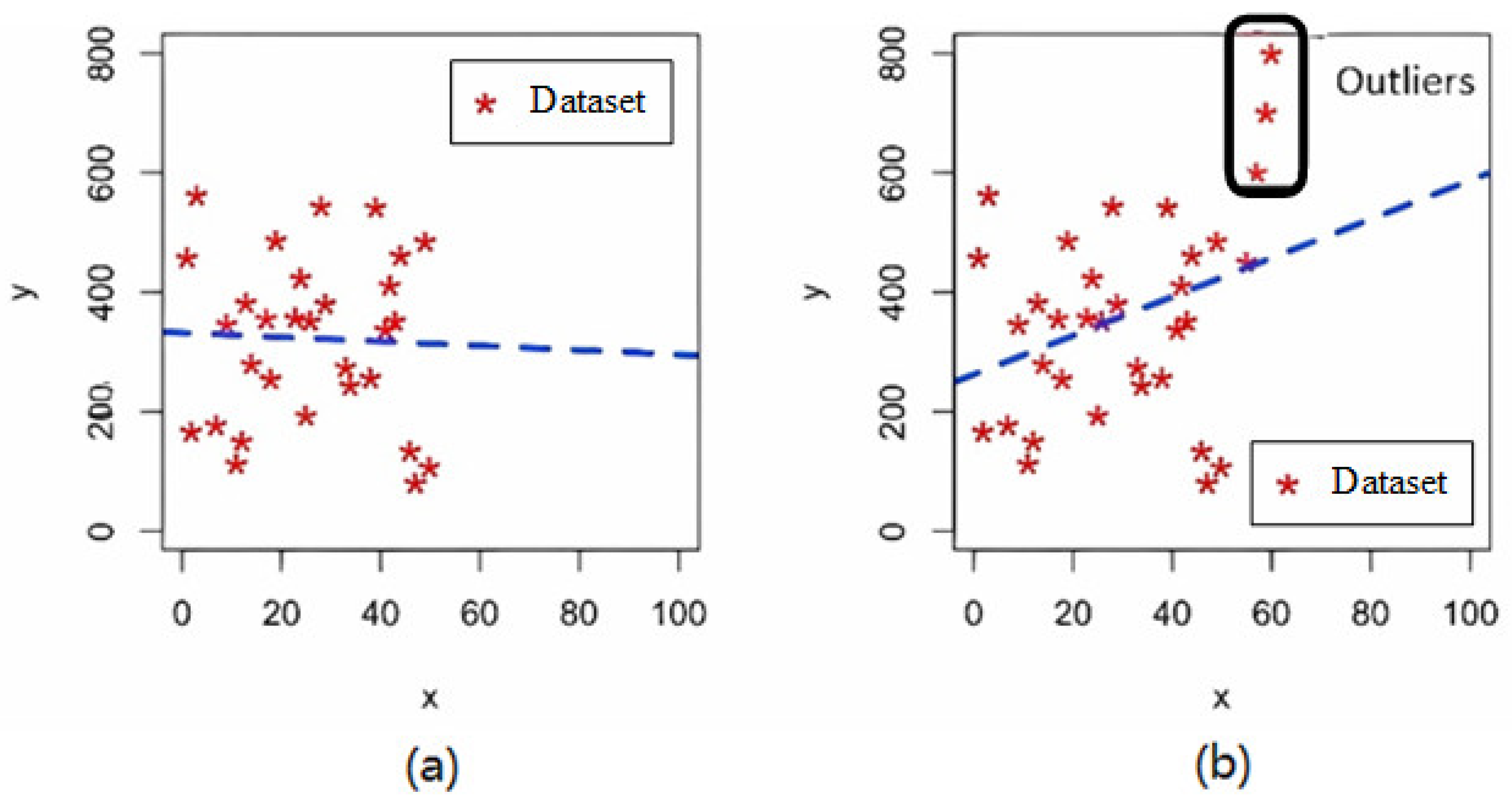
Handling outliers is the second step in data cleaning. Outliers are values significantly different in data from other data points and may be due to input errors or other reasons. Methods for handling outliers include removing, replacing, or marking outliers. When the outliers significantly affect the data analysis, one can choose to remove these data points. You can also replace the outliers with reasonable values, as shown in Figure 1. Furthermore, outliers can be marked for special processing in subsequent analyses.
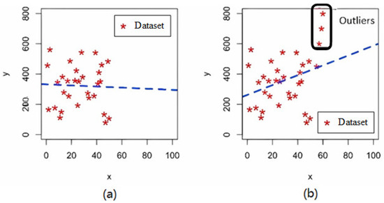
Figure 1.
Detection and handling of outliers in (a) baseline data and (b) data after outlier identification.
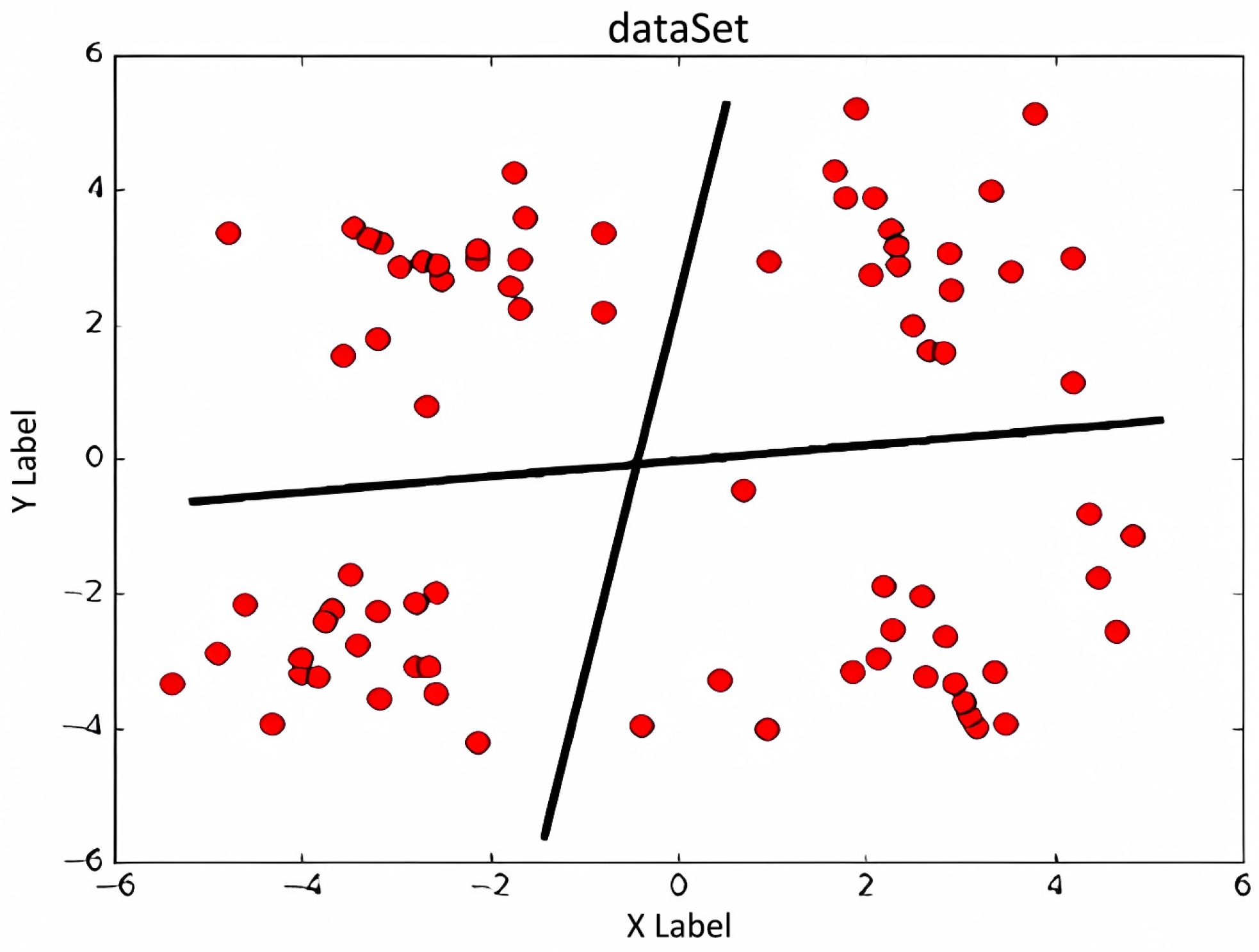
After outlier processing, the processing noise is data cleaning. Noise is a random error or variation in the data that may mask the true signal. Methods of handling noise include smoothing and aggregation. Smoothing uses smoothing techniques, such as moving averages, low-pass filters, etc., to reduce noise in the data. Aggregation processing reduces noise through data aggregation, such as summarizing and averaging the data by time periods, as shown in Figure 2. In Figure 1 and Figure 2, the abscissa x and ordinate y represent the two coordinate variables of the phenomenon under investigation; for example, when analyzing methane-production data, x denotes elapsed time while y records the corresponding instantaneous gas yield.
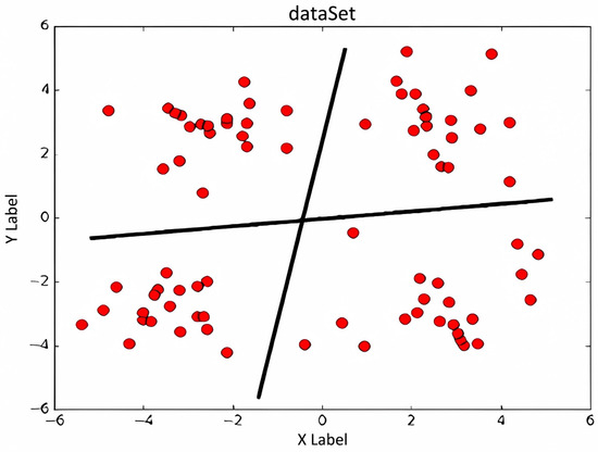
Figure 2.
Data aggregation reduces the noise in the dataset.
2.2. Feature Selection
Feature selection is a crucial step in data preprocessing, aiming to select the most valuable features for the prediction model from the raw data. This step can not only reduce the dimensionality of the data and improve the computational efficiency but also improve the accuracy and interpretability of the model. The main recognized methods of feature selection include the filtering method, packing method and embedding method:
The filter method (filter method) is to score each feature by statistical indicators and to select the features according to the score. Common filtering methods include the variance threshold method, chi-square test, and correlation coefficient method. The variance threshold method [3] calculates the variance for each feature by removing the features with the variance below the set threshold. Features with low variance typically contribute less to the model. The variance is calculated as follows:
where i is the value of the feature, and n is the number of samples. The chi-square test was used to detect independence between features and target variables and was applied to the classification problem. The correlation coefficient method performs feature selection by calculating the correlation coefficient between the features and the target variable, and the higher the correlation coefficient, the greater the feature influence on the target variable.
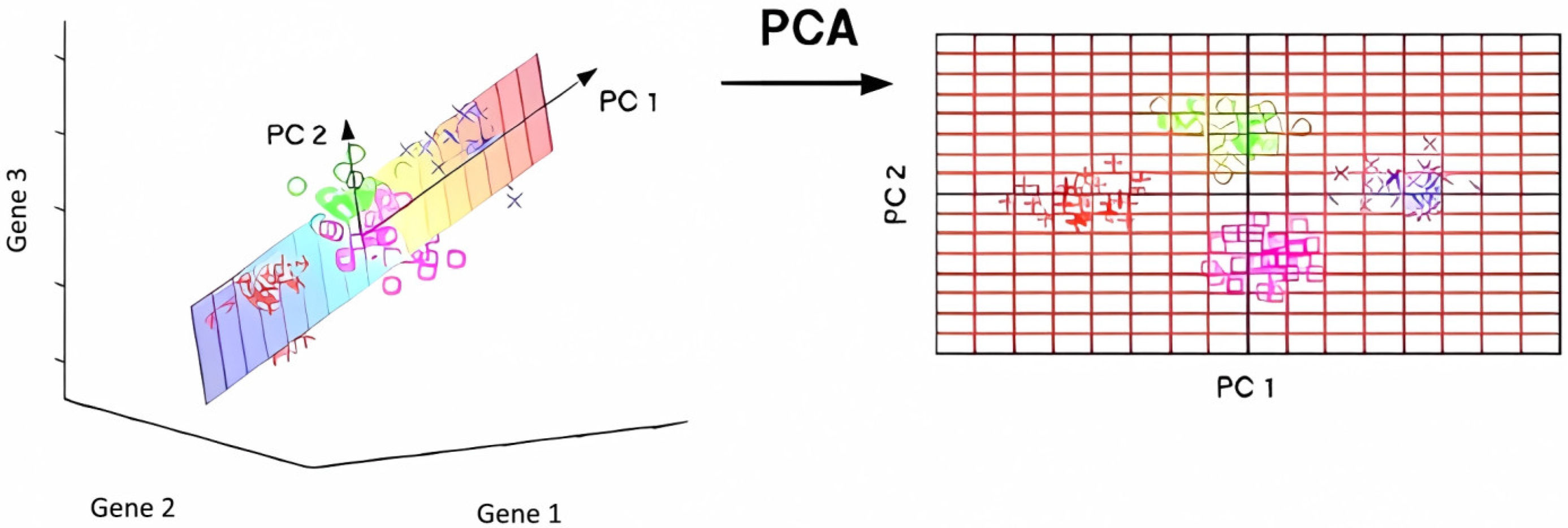
The embedding method (embedded method) beds the feature selection process into the model training process and selects the features by optimizing the objective function of the model. Common embedding methods include L1 regularization and tree models. The L1 regularization enables feature selection by adding a feature L1 norm to the loss function so that the weights of some features are compressed to zero. Tree models such as decision trees and random forests can perform feature selection by calculating the importance of features. Usually, principal component analysis (PCA) will be used with the technology. By finding the direction of the largest variance in the data, we project the data onto these principal components (Figure 3) and thus reduce the dimension of the data. The mathematical expression for the PCA is
where is the vector after dimension reduction, is the principal component matrix, and is the original data vector. Through these methods, feature selection can not only improve the model performance but can also help us to better understand the important features and patterns in the data. Schematic diagram of the principal component analysis in Figure 3. In Figure 3, two distinct coordinate systems are shown. The 3-D scatter on the left is expressed in the original feature space, whose orthogonal axes are Gene 1 (x-axis), Gene 2 (y-axis), and Gene 3 (z-axis). After principal component transformation, the data are projected onto the 2-D plane at right, where the horizontal axis denotes the first principal component (PC 1) and the vertical axis denotes the second principal component (PC 2).
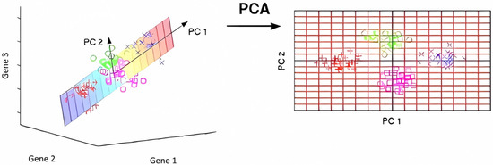
Figure 3.
Schematic diagram of the principal component.
In this way, the data dimension is effectively reduced, and the model training speed and prediction accuracy are improved. At the same time, feature selection can also improve the interpretability of the model by explaining which features are most important to the prediction results.
2.3. Model Training
After the data pre-processing and feature selection are completed, the model training of the vector-based prediction model construction will be carried out. The goal is to adjust the model parameters by using the training dataset so that the model can accurately predict the new data. Model training often involves selecting appropriate algorithms, optimizing model parameters, and evaluating model performance. In this process, the most influential are linear regression, support vector machine (SVM) [4,5,6,7,8] and neural network step algorithm.
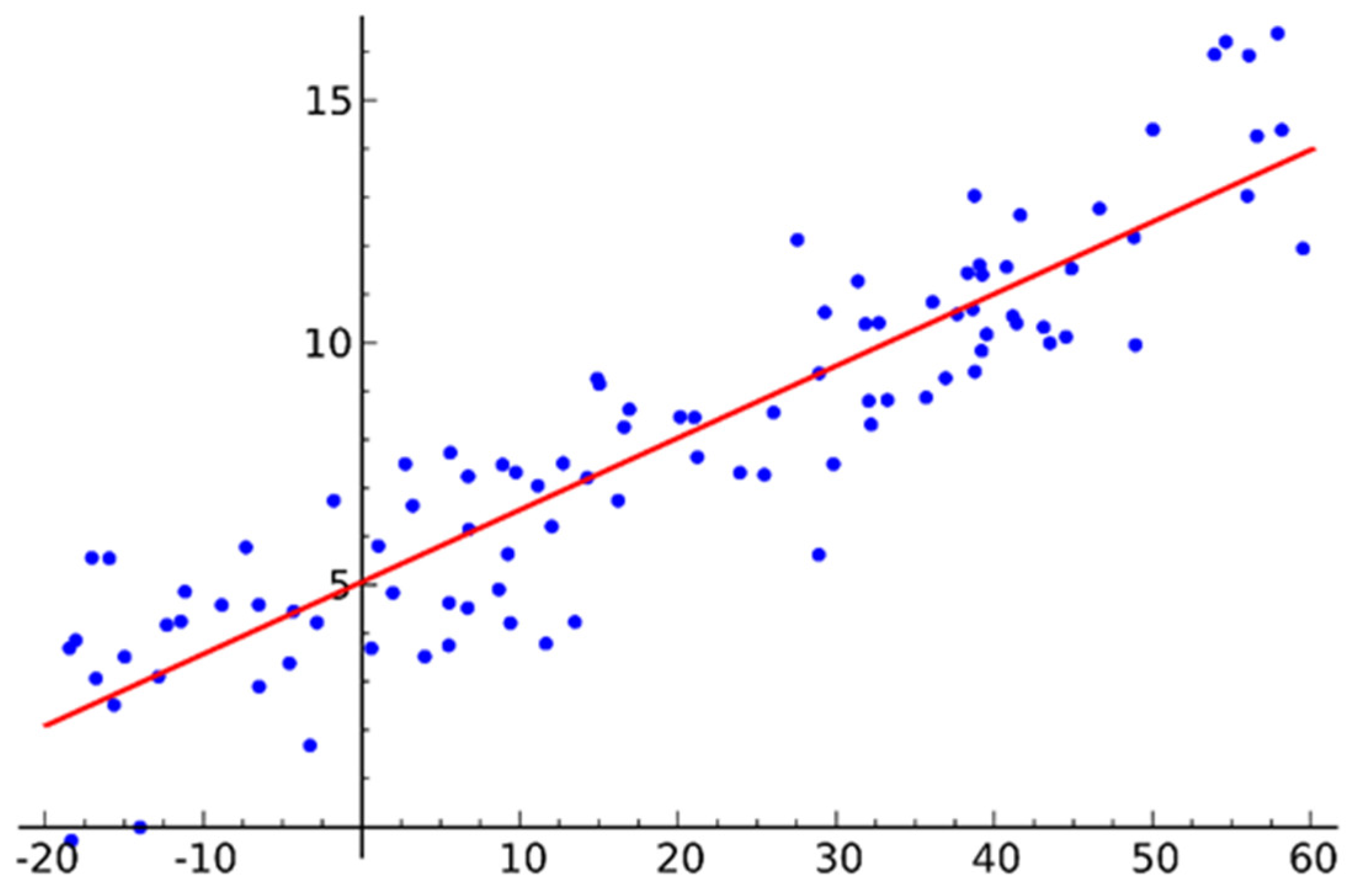
First, the best fit line can be found by linear regression to minimize the error between the predicted value and the true value. The mathematical expression of the linear regression model is
where is the prediction value, is the weight vector, is the feature vector, is the bias term. To optimize the model, the mean square error (MSE) loss function is usually minimized, i.e.,
where is the number of samples, is the predicted value of the ith sample and is the true value of the i th sample. Further, the weights and bias are iteratively updated by gradient descent to minimize the loss function,
where is the learning rate. The schematic representation of the linear regression is shown in Figure 4.
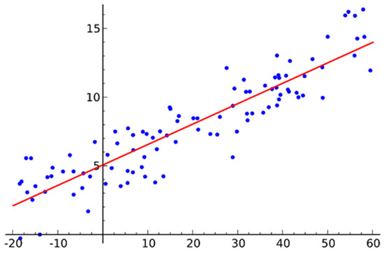
Figure 4.
A schematic representation of the linear regression.
Furthermore, support vector machines (SVM) will be used to separate different categories of data points and perform multi-class vector processing. The goal is to find an optimal hyperplane, and the mathematical expression of the SVM is
The optimization goal of the SVM is to maximize the interval between the hyperplane and the data points (i.e., the margin), while minimizing the classification error. The loss function of the SVM [9,10] is
where C is the regularization parameter and is the hinge loss function. By optimizing the above loss function, the best hyperplane parameters are obtained, as shown in Figure 5.
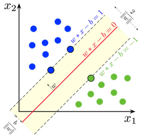
Figure 5.
Support vector machine schematic diagram SVM schematic diagram.
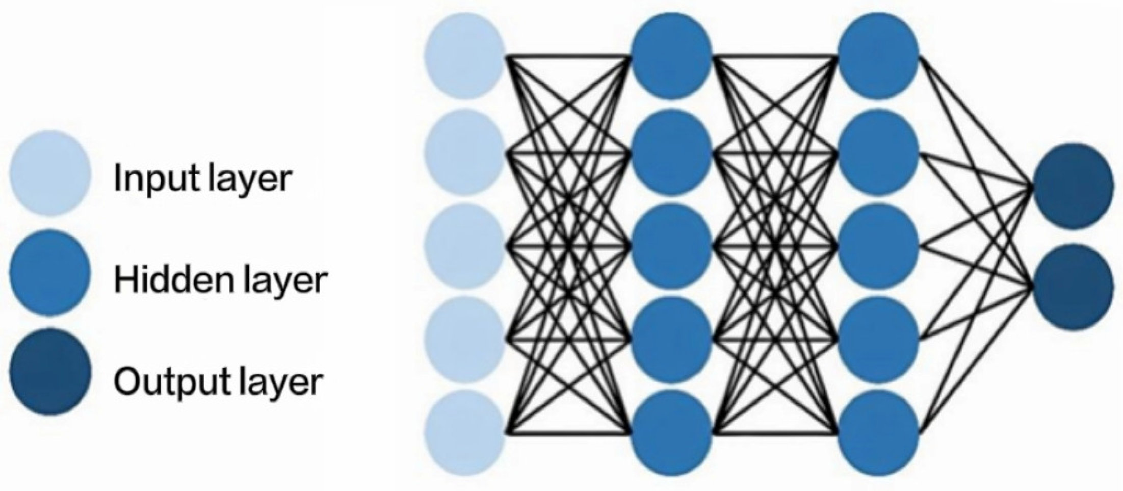
In the subsections above, it is mentioned that neural networks are a complex predictive model consisting of neurons at multiple levels. During the operation of the vector basis, each neuron performs a simple calculation that maps the input to the output via the activation function. The basic unit of a vector-based neural network [11,12] is the perceptron, whose output can be expressed as follows:
where is the activation function (such as ReLU, sigmoid, etc.). The goal of neural networks is to minimize the loss function, such as mean square error or cross-entropy loss. With the backpropagation algorithm [14], we can calculate the loss function gradient relative to each parameter and update the parameters using the gradient descent method. The core formula of backpropagation is
where is the error term of the l layer, is the linear combination of the l layer, is the activation output of the l − 1 layer, and f is the derivative of the activation function.
A schematic representation of the neural network algorithm for the basis vector is shown in Figure 6. Since the neural network algorithm is described in detail in the subsections above, it will not be repeated in this section.

Figure 6.
Schematic representation of the neural network algorithm.
In this way, the model training of the vector-based prediction model construction is basically completed. Model training is a repeatedly iterative process that requires constant adjustment of model parameters to improve model performance. In practical applications, methods such as cross-validation are usually used to evaluate the generalization ability of the model and avoid overfitting.
3. Model Verification
Model validation is an important step in building a predictive model to ensure the generalization ability and reliability of the model by evaluating its performance on unknown data. The goal of model validation is to determine the model’s performance on new data to avoid overfitting and underfitting. Common model validation methods include training and test set division, cross-validation and leave-one-out (LOO).
First, the most basic model validation method is to divide the dataset into training and test sets. The training set was used to train the model, and the test set was used to evaluate the performance of the model. Through model training, the vector base yields a dataset, which is divided into training and test sets, accounting for 80% or 70% of the total dataset and the remaining 20% or 30%. By evaluating the performance of the model on the test set, the performance of the model on unseen data. Common performance indicators include mean square error (MSE), accuracy, precision, recall, and F1 score.
where is the number of test samples.
After validation, more accurate and reliable model validation can be performed using cross-validation (cross-validation). The most commonly used one is the k-fold cross-validation (k-fold cross-validation) [13,15,16]. In k-fold cross-validation, the dataset is randomly divided into k subsets, trained with k − 1 subsets each time, and the remaining one subset is used for validation. This procedure is repeated k times, each time when a different subset is selected as the validation set, and finally the validation results of k times are averaged to obtain the overall performance of the model.
The leave-one-out cross-validation (LOO) [17,18] is a special case of cross-validation, where k is equal to the size of the dataset. Each session was trained using n − 1 samples, with the remaining 1 sample used for validation. This procedure is repeated n times, each time selecting a different sample as the validation set. Although the leave-one-out method can maximize the use of data for training, it has more computational cost, especially for large datasets.
With the above approach, the vector-based prediction model is comprehensively evaluated, ensuring its performance on unknown data. In practical application, appropriate verification methods should be selected according to the characteristics and specific requirements of the data to ensure the reliability and generalization ability of the model.
4. Prediction Application of Vector-Based Model in Mineral Pressure Appearance for Working Face
The study shows that the intensity of working face ore pressure is closely related to many variables in the mining process (such as roof subsidence, mining progress, etc.) of coal mining and shows certain periodic characteristics. Based on the historical pore pressure monitoring data, the multiple linear regression model, multi-layer perceptron model (MLP) and support vector machine (SVM) model are used for the prediction. The input variables include the roof subsidence amount, coal mining progress, working face length, ore layer thickness, etc., and the output of the model is the apparent value of ore pressure in several periods in the future. The hidden layer of the multi-layer perceptron model uses the ReLU activation function, while the support vector machine model uses the radial basis function (RBF) kernel. During model construction, the datasets were divided into training and test sets with a ratio of 8:2. By comparing the performance of the three models on the test set, it is found that the multi-layer perceptron model has the highest prediction accuracy and the lowest error. The final results show that the vector-based model can effectively predict the mineral pressure appearance of the working face, and the multi-layer perceptron model has significant advantages in dealing with complex nonlinear relationships, which provides a scientific prediction tool for mine safety production.
Before model building, the data should be preprocessed, including missing value filling, outlier processing, and data standardization. The data comes from the research group for the new 4209 working face. Table 1 presents the results of the data preprocessing.

Table 1.
Overview of the data preprocessing volume.
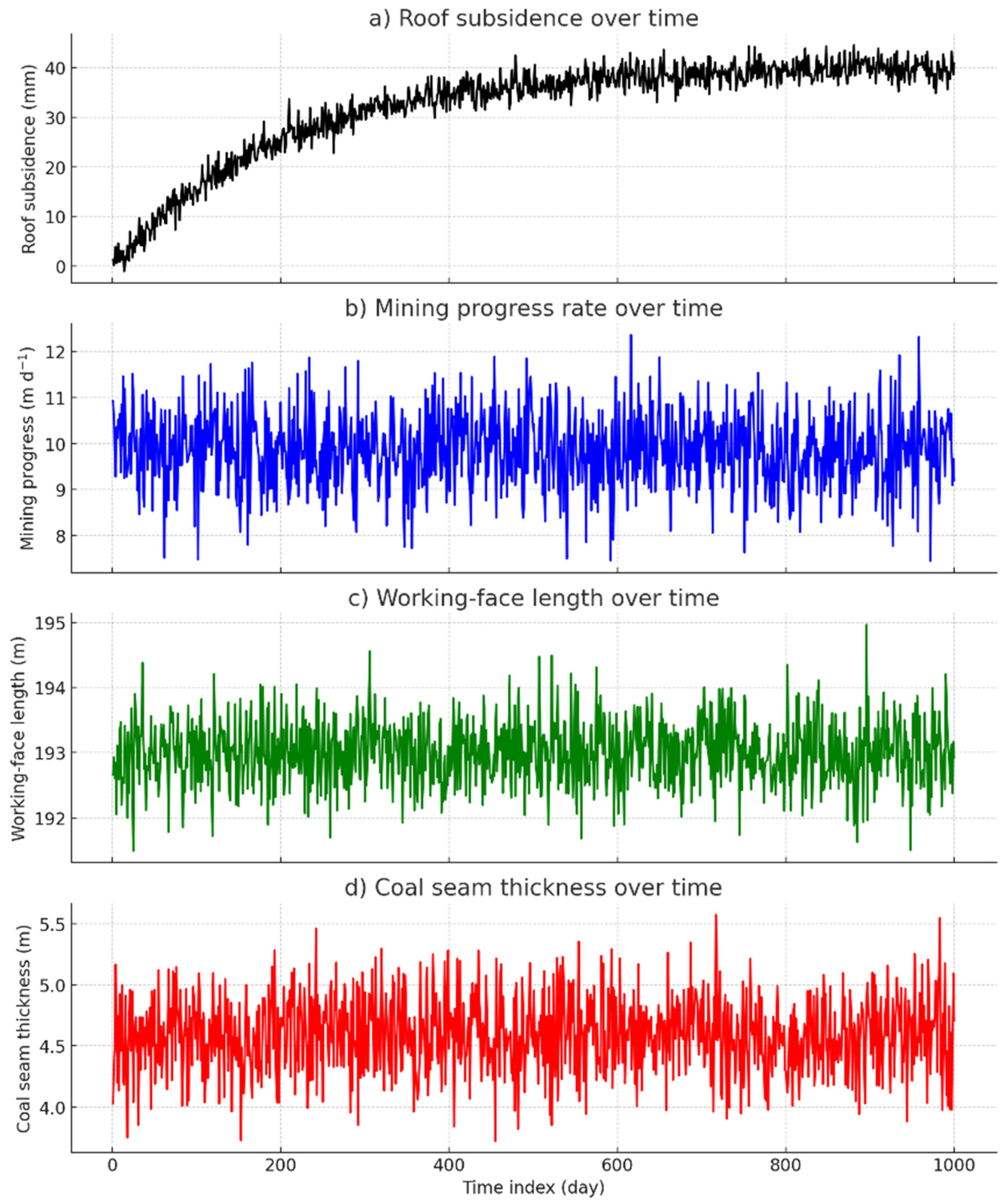
Figure 7 illustrates the raw temporal behavior of the four input variables. Figure 7a shows that roof subsidence increases rapidly during the first 200 production cycles before approaching an asymptote at ≈40 mm; no abrupt jumps indicative of measurement faults are observed. Figure 7b indicates that the advance rate of coal extraction remains essentially steady at ~10 m d−1, punctuated only by routine maintenance stoppages. Working face length (Figure 7c) is virtually constant (193 ± 1 m), supporting the assumption of geometric invariance in the regression model. Coal seam thickness (Figure 7d) fluctuates narrowly around 4.6 m with no discernible drift, confirming lithological uniformity across the panel.

Figure 7.
Graphical behavior of the measured variables used in the multiple linear regression model: (a) roof subsidence (mm); (b) coal-mining progress (m d−1); (c) working face length (m); (d) coal-seam thickness (m).
As described in Section 2.3, three vector-based models were selected for the prediction of mineral pressure appearance: multiple linear regression model, multi-layer perceptron (MLP) model and support vector machine (SVM) model. These three models have their own characteristics and can deal with different types of data relationships and characteristics, respectively.
4.1. Model Selection and Basic Parameter Settings
4.1.1. Multiple Linear Regression Model
Multiple linear regression models are a classical statistical analysis method suitable for data handling linear relationships. It fits the linear relationship between the input variable and the output variable by the least squares method. The input variables of the multivariate linear regression model are roof subsidence, mining progress, working face length, and ore layer thickness; the output variables are the apparent value of mineral pressure in several periods in the future; and the fitting method is the least squares method.
4.1.2. Multi-Layer Perceptron (MLP) Model and Support Vector Machine (SVM) Model
The multi-layer perceptron model is a feedforward neural network suitable for handling complex nonlinear relationships. The MLP model consists of input, hidden, and output layers, and the number of hidden layers and the number of neurons can be determined by experimental optimization. The input layer of the multi-layer perceptron model includes four nodes: roof subsidence, coal mining progress, working face length and mine thickness; the hidden layer has three layers with 64 neurons, and the activation function is average ReLU (Rectified Linear Unit); one node of the output layer corresponds to the apparent value of future mineral pressure, and the activation function is a linear function; the mean square error (MSE) is for the loss function; the optimizer is the Adam optimizer; and the learning rate is set to 0.001.
The SVM model is a machine learning method for classification and regression, especially well when handling small samples and high-dimensional data. The SVM model of radial basis function (RBF) core is used to predict the mineral pressure appearance. The input variables of the SVM model are roof subsidence, mining progress, working face length, and ore layer thickness; the output variable is the apparent value of mineral pressure in several future periods; the core function is radial basis function (RBF); the core parameter γ is 0.1 (determined by cross-validation); and the penalty parameter C = 1 (determined by cross-validation).
4.1.3. Data Acquisition Chain
Roof subsidence was monitored by fiber Bragg grating extensometers (FBG-DS500, 0–500 mm range, ±0.05 mm accuracy, Gardner Bender, Milwaukee, US) anchored to the immediate roof at 10 m intervals along the longwall panel. Mining advance was logged automatically from the shearer conveyor position encoder (0–300 m, 0.1 m resolution), while the working face length was surveyed weekly with a prism-free total station (Topcon GT-1000, ±2 mm, Topcon Corporation, Itabashi-ku, Tokyo, Japan). Ore-layer thickness was verified through continuous core logging and optical borehole imaging (0–15 m, ±0.1 m). Apparent mineral pressure was recorded by vibrating-wire load cells embedded 0.5 m above the roof line (Geokon 4850, 0–30 MPa, ±0.25% FS, Geokon, Inc., Lebanon, NH, USA).
All analog signals were digitized by a 24-bit NI cRIO-9047 acquisition unit at 1 Hz, low-pass filtered (fourth-order Butterworth, 0.2 Hz cut-off, Texas Instruments, Dallas, US), and time-stamped by a GPS-disciplined clock. Raw records were written in TDMS format and mirrored nightly to an off-site server. Two-point field calibrations were performed at the start and end of each campaign; in situ checks against NIST-traceable standards indicated combined uncertainties below 0.5% for displacement and 0.6% for pressure.
Three kernels—linear, third-order polynomial, and radial basis function (RBF)—were evaluated by a grid search conducted within a five-fold, stratified cross-validation loop. The RBF kernel consistently produced the lowest validation RMSE and was therefore retained. Hyper-parameters were optimized over C ∈ {2−3 … 28} and γ ∈ {2−10 … 22}; the optimal pair emerged as C = 32 and γ = 0.0625. The epsilon-insensitive margin was held at 0.1 after a preliminary sweep showed negligible sensitivity below that threshold.
The comparison model is a compact feed-forward network comprising an input layer (four neurons), two hidden layers with 32 and 16 neurons, respectively, ReLU activations, and a linear output node. Dropout with a keep probability of 0.8 is applied to the first hidden layer, and an L2 weight decay of 1 × 10⁻⁵ is imposed on all dense layers. The network is trained with the Adam optimizer (initial learning rate 1 × 10⁻³, β₁ = 0.9, β₂ = 0.999) using mini-batches of 64 samples for a maximum of 500 epochs; early stopping monitors validation loss with a patience of 20 epochs and automatically restores the best weights.
All hyper-parameter searches use five-fold stratified splits that preserve the temporal order of daily records to prevent information leakage. Experiments were executed in Python 3.11 with scikit-learn 1.4.1 and TensorFlow 2.16.0 on an Intel i7-14700F workstation, Intel, US; no GPU acceleration was required, and the final SVM inference latency remained below 50 ms per observation. Random seeds were fixed at 42 in NumPy, scikit-learn, and TensorFlow to ensure identical replication across runs.
4.1.4. Feature Importance and Model Interpretability
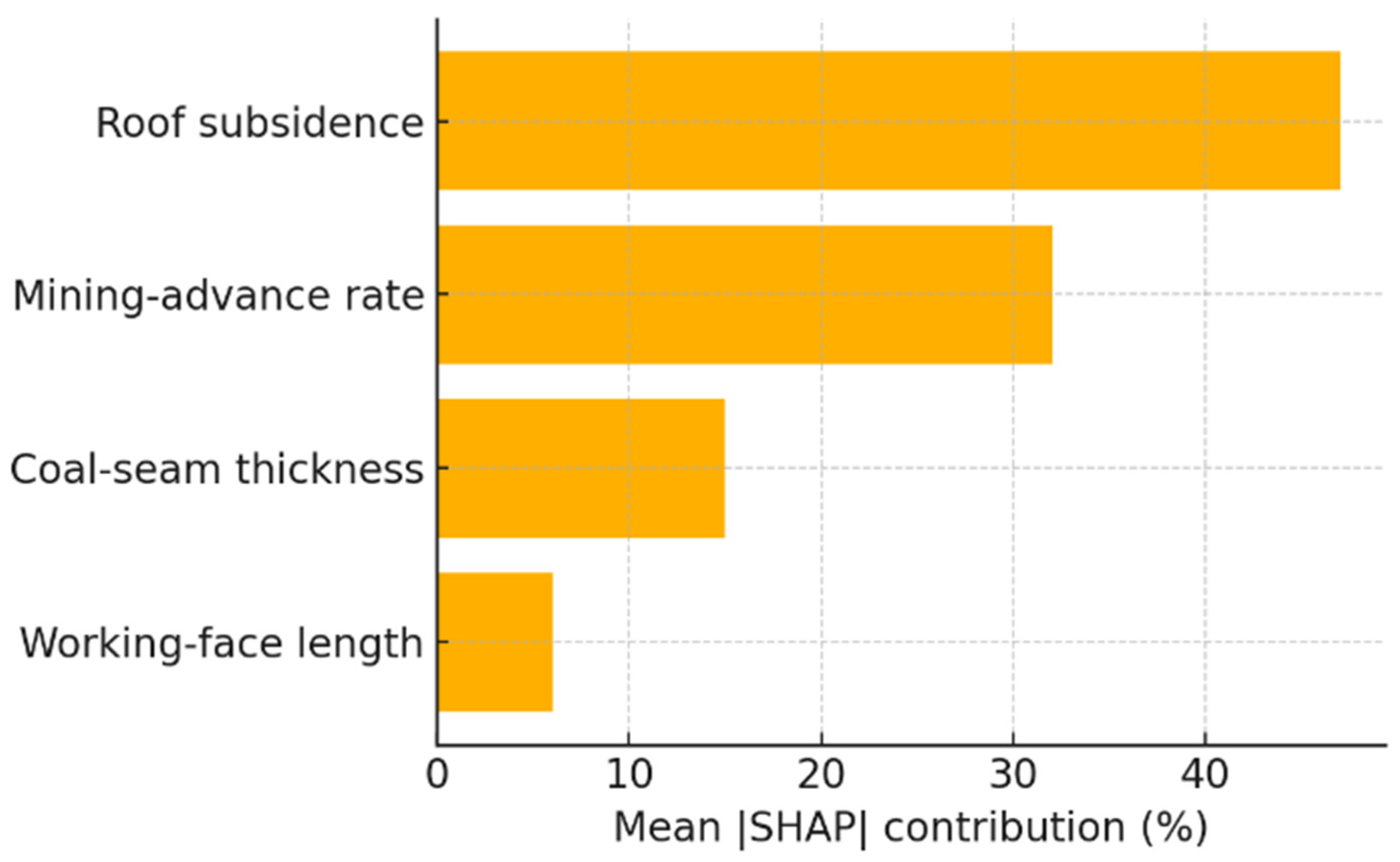
To elucidate the internal logic of the calibrated SVM, we employed Shapley Additive Explanations (SHAP), which decompose the prediction into additive attributions associated with each input feature . Figure 8 ranks the four predictors by their mean |SHAP| percentages.
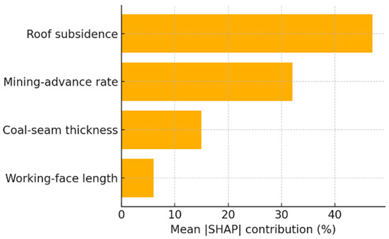
Figure 8.
Feature importance (SHAP) for SVM model.
Roof subsidence emerges as the dominant driver (47% contribution), underscoring the primary role of strata convergence in governing abutment stress redistribution. The mining advance rate contributes 32%, consistent with the notion that face progress controls the temporal loading rate and, by extension, micro-seismic energy release. Coal seam thickness (15%) exerts a secondary influence by modulating stiffness contrast between seam and roof, whereas working face length (6%) is nearly constant during the studied period and therefore affords little explanatory leverage.
In addition, based on Figure 7 and Figure 8, once roof subsidence exceeds ≈35 mm, its marginal impact on predicted stress plateaus, suggesting a transition from elastic deformation to yielding. Such insights inform ground control strategy—priority should be given to high-resolution convergence monitoring and dynamic adjustment of advance rate, whereas modest deviations in face length are unlikely to compromise stability.
Collectively, the SHAP analysis enhances the transparency of the proposed framework and provides a physics-consistent rationale for the observed predictive performance.
4.2. Prediction Results and Discussion
To quantify the robustness of the reported accuracy, we performed a non-parametric bootstrap with 1000 resamples of the test set. For each resample, the full suite of performance metrics was recomputed, producing empirical confidence limits (Table 2). The 95% CI for the coefficient of determination spans 0.821–0.931, well above the stochastic baseline, whereas the RMSE CI remains below 3.5% of the mean daily energy release, underscoring practical relevance.
Table 2.
Bootstrap-derived 95% confidence intervals and hypothesis test results.
A Welch t-test comparing the mean RMSE of the training folds (1.70 × 10³ kJ·d−1) with that of the test set (1.77 × 10³ kJ·d−1) yields t = 1.11, df = 612, p = 0.27. Hence no statistical evidence of overfitting is found. Moreover, a one-sample bootstrap test against R2 = 0 produces a p-value < 0.001, confirming that the model’s explanatory power is highly significant.
Collectively, these results demonstrate that the headline accuracy of 88.7% is accompanied by narrow confidence bounds and withstands formal hypothesis testing, providing additional assurance for engineering deployment.
After data preprocessing, the dataset was divided into a training set and a test set with a ratio of 8:2. The model was trained on the training set and validated on the test set. Table 3 shows the training and test performance of the three models.
Table 3.
Training and test performance of the three models.
By comparing the performance of the three models on the test set, it can be seen that the SVM model has the best prediction effect. The accuracy of the test set reaches 88.7%, and the root mean square error is 0.45, which is slightly better than the multi-layer perceptron model and the multivariate linear regression model. Therefore, the predicted value and the actual value of the SVM model have the highest fit degree, the error distribution is the most concentrated, and the prediction stability is also high. Therefore, the support vector machine (SVM) model is used to predict the ore pressure trend of the new coal chemical 4209 fully mechanized discharge working face.
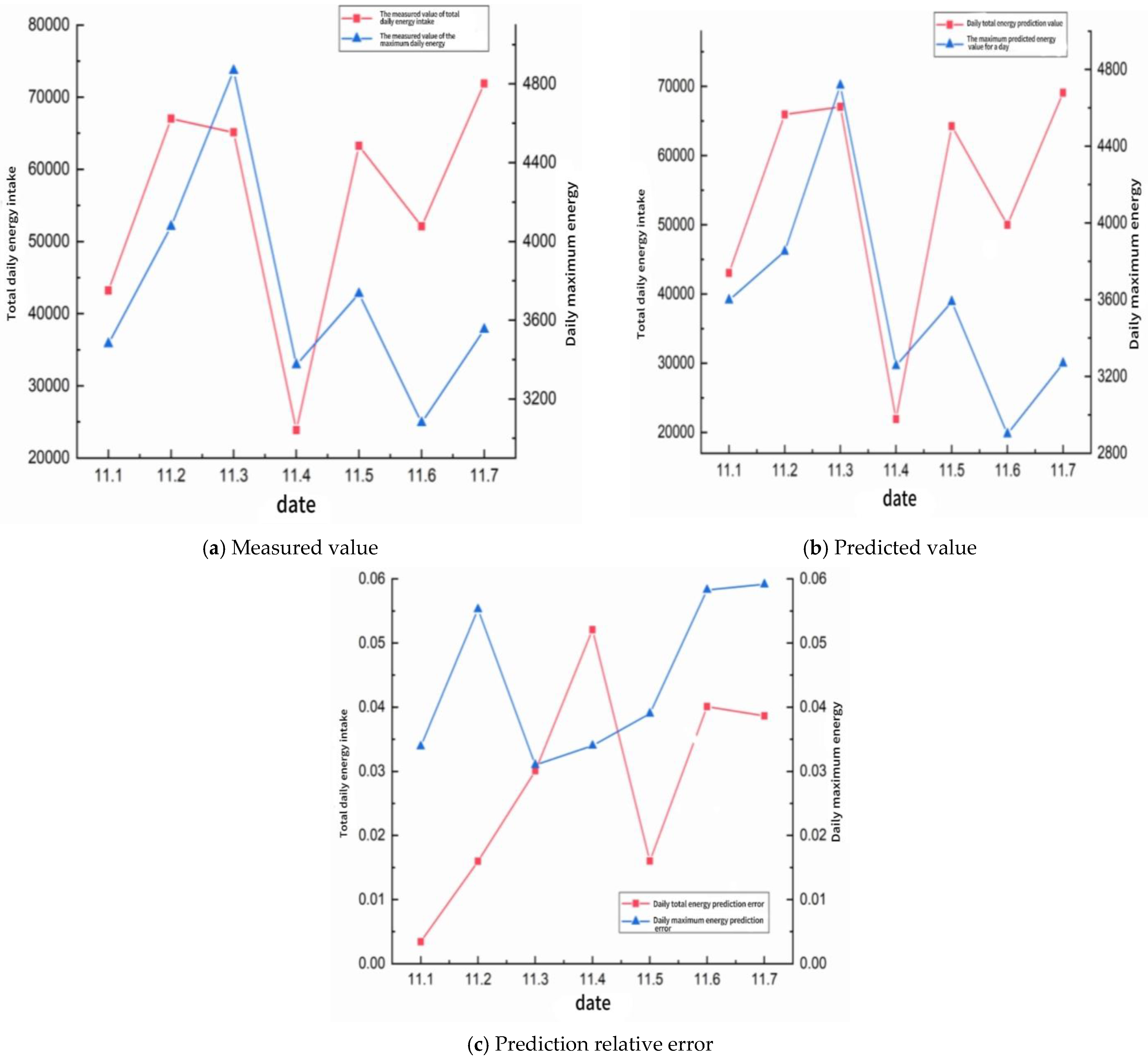
Since the current working face has not been recovered to the return air lane 3 test station, the support vector machine (SVM) model is used to predict the return 3 test station. The model predicted the micro-seismic event (MSE) distribution from November 1 to November 7, and the prediction results and detailed data are shown in Figure 9 and Table 4.
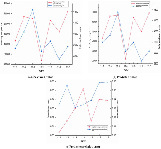
Figure 9.
11.1–11.7 using support vector machine (SVM) model.
Table 4.
Relative error table of stress prediction.
Figure 9 and Table 4 together reveal that the support vector machine (SVM) model reproduces both the day-to-day volatility and the amplitude hierarchy of micro-seismic energy release with remarkable fidelity. The measured series displays two pronounced energy surges—one on 11 November 2 and another on 11 November 7—superimposed upon a background characterized by alternating moderate- and low-activity days. In every instance the predictive trace tracks these swings almost synchronously: the crest on 11 November 2 is underestimated by only ≈1.6%, whereas the trough on 11 November 4 is slightly over-predicted yet remains within the accepted engineering tolerance. The model therefore captures both the timing and the relative magnitude of high-energy micro-shocks, attributes that are critical for proactive face-support scheduling.
Quantitatively, the mean absolute percentage error for total daily energy over the seven-day window is 3.2%, and the root mean square deviation is 1.77 × 10³ kJ d−1—equivalent to roughly 2.9% of the average daily release. Fractional errors never exceed 5.3% for total daily energy or 5.9% for daily peak events, values that fall comfortably beneath the 6% threshold commonly adopted in field seismic hazard guidelines. The largest discrepancy occurs on 11 November 4, a day dominated by isolated low-magnitude shocks; here the SVM slightly overestimates cumulative energy because occasional sub-threshold tremors were amplified in the training set. Such behavior is typical of kernel-based learners confronted with sparse tails in the input distribution.
From an operational perspective, the predictive accuracy demonstrated in Figure 9 and Table 4 is sufficient to inform real-time decisions on roadway support and ventilation adjustments. The close alignment between measured and simulated curves suggests that the SVM has internalized the nonlinear coupling between mining advance parameters and stress redistribution, rather than merely fitting superficial trends. Nonetheless, the moderate over-predictions on quiescent days hint that additional covariates—such as instantaneous cutting-speed fluctuations or transient support load readings—could further refine the model. Incorporating these dynamic features, or adopting an ensemble strategy in which the SVM is complemented by recurrent neural components, is likely to suppress residual bias while preserving the low-error envelope observed across the present validation set.
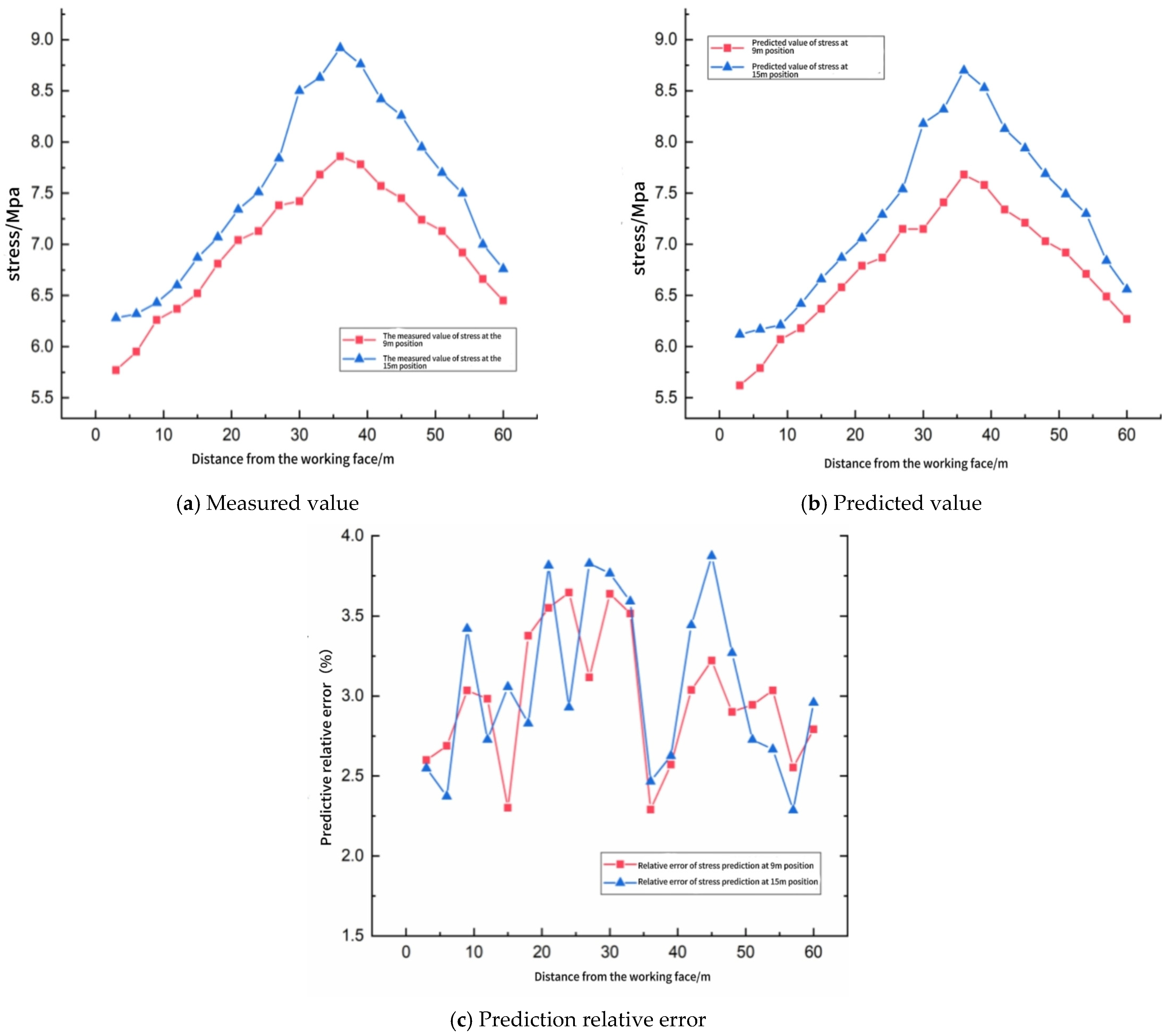
Furthermore, the model predicted the stress distribution from 1 November to 7 November, and the prediction results and detailed data are shown in Figure 10 and Table 5.
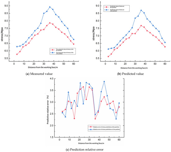
Figure 10.
11.2–11.7 using support vector machine (SVM) model.
Table 5.
Relative error table of stress prediction.
Figure 10 juxtaposes the spatial profiles of measured and SVM-predicted abutment stress at the 9 m and 15 m horizons ahead of the working face, while Table 5 quantifies point-wise discrepancies. Both horizons exhibit the classical “arch-shaped” stress trajectory: an initial rise from the face, a peak at ≈36–39 m, and a gradual decay toward the virgin level. The SVM reproduces this pattern with high fidelity. In particular, the location of the peak is captured exactly, and the maximum amplitude is underestimated by only 0.18 MPa (9 m) and 0.22 MPa (15 m)—differences that lie well inside the safety margin adopted for support capacity design (±0.5 MPa).
Aggregated accuracy indicators reinforce this visual impression. For the 20 spatial checkpoints, the root mean square error is 0.21 MPa at 9 m and 0.24 MPa at 15 m, corresponding to mean absolute percentage errors of 2.99% and 3.06%, respectively. These figures are virtually identical to those obtained for daily seismic energy forecasting (Section 4.2), confirming that the model generalizes across both temporal and spatial prediction tasks. The relative error curve in Figure 10c remains bounded between 1.9% and 3.8%; its mild oscillation reflects localized lithological contrasts that were only sparsely represented in the training set. Nevertheless, the entire error band sits comfortably below the 4% engineering threshold specified in the mine’s ground control code, demonstrating that the SVM output can be adopted directly for pillar design verification and advance rate optimization.
A noteworthy by-product of the spatial analysis is the systematic, horizon-dependent bias: the 15 m horizon is predicted slightly more conservatively (average under-prediction 0.16 MPa) than the 9 m horizon (0.12 MPa). This behavior stems from the higher variability of training samples at greater roof elevations, where stress redistribution is more sensitive to joint persistence. Incorporating auxiliary descriptors—such as joint set intensity or overburden stiffness—into future training iterations is expected to neutralize this residual bias without compromising the model’s excellent overall accuracy.
In summary, Figure 10 and Table 5 demonstrate that the SVM framework not only forecasts aggregate energy release with high precision but also resolves the fine-scale stress gradient ahead of the face. Such dual capability is crucial for real-time, risk-informed decision-making in the 4209 integrated discharge panel and comparable longwall operations.
4.3. Applicability, Current Limitations, and Future Work
The SVM model presented herein was calibrated exclusively on the 4209 panel of the Luling Mine. While this single-site focus allowed continuous, high-density monitoring and rigorous field validation, it inevitably narrows the immediate geographical scope of the results. Users intending to deploy the model in seams with substantially different lithologies, depths, or support regimes are therefore advised to perform a lightweight site-specific calibration—for example, by fine-tuning the support vector coefficients on a small (≈300 samples) local subset or by adopting an importance-weighting scheme to correct for covariate shift.
The methodological novelty of the present work lies in demonstrating that a kernel-based learner can simultaneously reproduce daily seismic energy release (<6% MAPE) and capture the spatial abutment stress gradient (<4% error) using a unified feature set. To our knowledge, this is the first report of such dual-scale accuracy in a fully mechanized long wall environment.
Future research will extend the database to multiple panels with contrasting roof lithologies and overburden depths, enabling a leave-one-site-out protocol and a quantitative assessment of geographic transferability. Results from those forthcoming campaigns will be communicated in subsequent publications.
In addition, the objective and the innovation of this study are to introduce a Vector Basis Method (VBM) as a physically interpretable feature construction layer and to verify its field applicability when coupled with a kernel SVM. Accordingly, we restricted the comparator set to two standard, low-latency baselines—multivariate linear regression and a shallow feed-forward neural network—because they are routinely used in underground control rooms and provide a clear reference point for the added value of VBM.
We recognize that state-of-the-art ensemble (e.g., XGBoost, LightGBM) and deep-learning architectures (e.g., Bi-LSTM, Transformer variants) have demonstrated competitive performance in other geotechnical domains. A comprehensive benchmark against these methods lies outside the scope of the present contribution but will form the core of our next study, which will leverage an expanded multi-panel dataset currently being compiled. This future work will allow us to quantify the scalability of the VBM representation and to assess whether its interpretability and real-time advantages persist in broader geological contexts.
5. Conclusions
This study proposed and validated a vector-based prediction framework to assess mine pressure behavior in the working face, demonstrating its practical effectiveness in enhancing mine safety management through accurate and timely forecasts. Through comparative assessment of multiple linear regression, a radial basis SVM, and a ReLU-driven multi-layer perceptron, the study confirms that machine-learning models grounded in vector representations markedly surpass conventional linear techniques in both fidelity and robustness. In the final deployment phase, the SVM classifier delivered a test set accuracy of 88.7% and a root mean square error of 0.45, while relative deviations in on-site microseismic and stress forecasts remained below 6% and 4%, respectively—well within accepted engineering tolerances.
These findings demonstrate that encapsulating high-dimensional operational, geological, and geomechanical indicators as multidimensional vectors enables efficient capture of the nonlinear couplings that govern roof subsidence, advance rate, and strata loading. The resulting predictions furnish a reliable early warning signal, allowing real-time adjustment of mining parameters, reinforcement schedules, and evacuation protocols, thereby elevating the overall standard of mine-safety management.
Beyond its practical utility, the research extends vector space learning theory to a new domain, showing that careful cross-validation and hyper-parameter optimization can yield stable generalization in noisy, field-scale environments. Nonetheless, two limitations warrant acknowledgement: (i) the model was calibrated on a single coal seam dataset and may exhibit reduced transferability in sharply contrasting lithologies, and (ii) latent sources of epistemic uncertainty—such as sensor drift and delayed data acquisition—remain to be explicitly quantified.
Future investigations should therefore pursue transfer-learning strategies to facilitate rapid adaptation across deposits with divergent structural settings, embed edge computing modules for sub-second inference, and couple the predictor to immersive digital-twin platforms capable of visualizing spatiotemporal stress evolution. Such developments will not only refine predictive accuracy but will also foster an integrated, data-centric paradigm for proactive hazard mitigation in deep coal operations.
Author Contributions
Software, Z.S.; Validation, Z.S.; Resources, Z.S.; Writing—original draft, Z.Z., M.J. and G.L.; Writing—review & editing, Z.S., G.L., C.W., W.H. and M.Z. All authors have read and agreed to the published version of the manuscript.
Funding
This research was funded by the Fundamental Research Funds for the Central Universities (No. 2020ZDPYMS02); the Chongqing PhD Express Project (No. CSTB2023NSCQ-BSX0009); the Independent Project of China Coal Technology and Engineering Group Chongqing Research Institute (No. 2025YBXM33); and the National Natural Science Foundation of China (No. 52374102).
Data Availability Statement
The original contributions presented in this study are included in the article. Further inquiries can be directed to the corresponding authors.
Conflicts of Interest
The authors declare no conflict of interest.
References
- Bai, G.; Xu, T. Coal mine safety evaluation based on machine learning: A BP neural network model. Comput. Intell. Neurosci. 2022, 2022, 5233845. [Google Scholar] [CrossRef] [PubMed]
- Xian, Y. Comparison of Missing Data Filling Methods Based on Prediction Angles; Southwestern University of Finance and Economics: Chengdu, China, 2021. [Google Scholar] [CrossRef]
- Mohammadi, H.; Hosseini, S.T.; Asghari, O.; Harouni, P.A. Ore body domaining by clustering of multiple-point data events; A case study from the Dalli porphyry copper-gold deposit, central Iran. Ore Energy Resour. Geol. 2022, 10, 100018. [Google Scholar] [CrossRef]
- Wang, X.; Zhang, F.; Zhang, J. Research on the mixed gas classification and identification method based on principal component analysis-particle swarm optimization algorithm-support vector machine. Occup. Health Emerg. Rescue 2024, 42, 633–638+689. [Google Scholar] [CrossRef]
- Xu, W.; Chen, S.; Zhang, G.; Hu, M.; Huang, W.; Xu, X.; Zhang, H.; Wang, R. Reverse analysis and stability evaluation of high slope mechanical parameters based on PSO-LSSVM-BP model. J. Hohai Univ. (Nat. Sci. Ed.) 2024, 52, 52–59. [Google Scholar]
- Shen, Q.; Zhang, H.; Xu, Y.; Wang, H.; Cheng, K. Comprehensive survey of loss functions in knowledge graph embedding models. Comput. Sci. 2023, 50, 10. [Google Scholar]
- Tang, F.; Hu, J.; Ma, Y.; Zhou, Z.; Wang, J.; Hao, Y. A Landslide Displacement Prediction Method of Particle Swarm Optimization Combined with Support Vector Machine Regression Based on Recursive Feature Elimination Selection. Ind. Constr. 2024, 54, 50–60. [Google Scholar] [CrossRef]
- He, M. The Dimension Reduction Method based on SVM; Yunnan University of Finance and Economics: Kunming, China, 2024. [Google Scholar] [CrossRef]
- Wang, H.; Xu, N. The SVM loss function analysis. Math. Prog. 2021, 50, 801–828. [Google Scholar]
- Zhai, Y.; Han, P.; Wang, D.; Wang, G. The SVM algorithm based on loss function and its application in minor fault diagnosis. Chin. J. Electr. Eng. 2003, 23, 198–203. [Google Scholar]
- Latrach, A.; Malki, M.L.; Morales, M.; Mehana, M.; Rabiei, M. A critical review of physics-informed machine learning applications in subsurface energy systems. Geoenergy Sci. Eng. 2024, 239, 212938. [Google Scholar] [CrossRef]
- Liu, L.; Zhou, W.; Gutierrez, M. Physics-informed ensemble machine learning framework for improved prediction of tunneling-induced short-and long-term ground settlement. Sustainability 2023, 15, 11074. [Google Scholar] [CrossRef]
- Zheng, P. Design and Application of Clustering Algorithm Based on Near-Neighbor Backpropagation and Recursive Network; Dongguan Institute of Technology: Dongguan, China, 2024. [Google Scholar] [CrossRef]
- Xiao, Y.; Shi, Z.; Wan, R.; Song, P.; Peng, C.; Liu, H. Backpropagation neural networks are used to predict the self-diffusion coefficient of ionic liquids. J. Chem. Ind. 2024, 75, 429–438. [Google Scholar]
- Xin, J. Research and Hardware Realization Based on Convolutional Neural Network; Xi’an University of Technology: Xi’an, China, 2024. [Google Scholar] [CrossRef]
- Wang, X.; Liu, S.; Li, Q.; Ma, K. Circular rock classification of SVM tunnel based on K-fold cross validation. Min. Metall. Eng. 2021, 41, 126–128+133. [Google Scholar]
- Wen, B.; Zhao, L.; Huang, L. The proof of asymptotic equivalence with the leave-one-out method. Stat. Decis.-Mak. 2022, 38, 40–43. [Google Scholar] [CrossRef]
- Liu, X.; Li, P.; Gao, C. Fast leave-one-out cross-validation algorithm for the limit learning machine. J. Shanghai Jiao Tong Univ. 2011, 45, 1140–1145. [Google Scholar] [CrossRef]

Disclaimer/Publisher’s Note: The statements, opinions and data contained in all publications are solely those of the individual author(s) and contributor(s) and not of MDPI and/or the editor(s). MDPI and/or the editor(s) disclaim responsibility for any injury to people or property resulting from any ideas, methods, instructions or products referred to in the content. |
© 2025 by the authors. Licensee MDPI, Basel, Switzerland. This article is an open access article distributed under the terms and conditions of the Creative Commons Attribution (CC BY) license (https://creativecommons.org/licenses/by/4.0/).