Abstract
The generation and propagation mechanisms of acoustic waves from leakage below the annular liquid level in gas wells have attracted widespread attention. To study the characteristics of acoustic sources beneath the liquid level, a physical model of leakage in the casing–tubing annulus was established by simulating the distribution patterns of the flow field and acoustic field within the annulus under tubing leakage conditions. Distinct from the traditional acoustic analysis of wellbore leakage in gas wells, this study focuses on acoustic waves generated by leaks located below the annular protection fluid level. It analyzes the flow regime and acoustic source characteristics beneath the liquid level under various operating conditions (including leakage aperture, velocity, and position). The research summarizes the evolution patterns of flow regimes when gas leaks into the annular protection fluid under different conditions and elucidates the generation mechanism of sub-liquid leakage noise and its propagation mechanism across the liquid surface. This work lays the theoretical foundation for detecting sub-liquid leakage at the wellhead using acoustic methods.
1. Introduction
Deep oil and gas resources serve as a crucial pillar for China’s energy production and infrastructure. However, under the influence of complex geological conditions, harsh production environments, and long-term corrosion/erosion, leakage in oil and gas well tubulars has become increasingly prominent. The resulting annular pressure poses a severe threat to production safety [1,2,3,4,5].
Currently, precise leak detection and localization both domestically and internationally primarily rely on logging technologies such as electromagnetic logging, ultrasonic logging, and noise logging [6,7,8]. These methods necessitate well shut-in operations, incurring high costs, long cycles, and consequently hampering production efficiency. Recent research indicates that analyzing leakage noise can enable the preliminary diagnosis of downhole leakage conditions. Among detection techniques, acoustic-method-based leakage detection is now widely applied in pipeline leak detection [9] and has emerged as a key research focus for the wellhead detection of casing–tubing leaks [10,11].
Regarding acoustic source characteristics, studies via simulation and experimentation have confirmed that acoustic waves from gas pipeline leaks result from the superposition of quadrupole and dipole sources. Under high-flow-rate conditions, quadrupole sources dominate, with energy concentrated primarily in the low-frequency band below 50 Hz [12,13]. Unlike the free diffusion of leak noise in pipelines, downhole leak acoustics are significantly constrained by the tubular structure. Research by Wang Qiong et al. on leaks in inner pipes within jacketed structures identified peak acoustic pressure phenomena at leakage orifices (jet noise) and near outer pipe wall boundaries. Lü Ningyi et al. [14], using Mohring’s acoustic analogy method, simulated casing–tubing leak sources and similarly concluded they are dominated by quadrupole and dipole sources. Critically, existing research predominantly focuses on gas-phase leakage scenarios, with studies on the acoustic characteristics of leaks below the annular protection fluid level remaining scarce.
Therefore, this study employed ANSYS 19.0 fluid simulation software to establish a model of tubing leakage beneath the annular protection fluid in gas wells. We systematically investigate the flow field distribution and acoustic wave propagation patterns, revealing the characteristics of the acoustic pressure field distribution. This work aims to provide a theoretical foundation for detecting sub-annular-fluid leakage at the wellhead using acoustic methods.
2. Methods
2.1. Selection of Multiphase Flow Model
The leakage of tubing gas into the annulus protection fluid constitutes a multiphase flow scenario and should be modeled using a multiphase flow approach. Widely used multiphase flow models in FLUENT include three categories: the Volume of Fluid (VOF) model, the Mixture model, and the Eulerian model [15,16,17,18]. As shown in Table 1, a comparative analysis was conducted to evaluate the advantages, features, and limitations of these three multiphase flow models. All three models are applicable to gas–liquid two-phase flow. However, the VOF model requires the volume fraction within each computational cell to sum to 1, implying no interaction or interpenetration between phases. This imposes stringent demands on grid quantity—even with high grid quality, insufficient grid resolution may lead to coexisting gas–liquid phases within individual cells. The Eulerian model involves computationally intensive and relatively unstable processes, primarily designed for particle tracking, and requires high-performance hardware. In contrast, the Mixture model is a simplified multiphase flow approach that accounts for interfacial penetration and slip between gas and liquid phases. Consequently, the Mixture model was selected for this study.

Table 1.
Comparative analysis of multiphase flow models.
2.2. Sound Field Simulation Method
Acoustic simulation methodologies primarily include the integrated acoustic model approach, the broadband noise model approach, and computational aeroacoustics (CAA) methods. The integrated acoustic model derives noise predictions through transient flow field calculations and time-varying pressure solutions, requiring prior flow field simulations, with the acoustic field inferred analogously from the flow field. Key acoustic analogy equations include the Ffowcs Williams–Hawkings (FW-H) equation and the Lighthill equation. The FW-H equation represents an improvement over the Lighthill equation, serving as a generalized form of Lighthill’s acoustic analogy method capable of modeling dipole and quadrupole noise sources. The broadband noise model approach [19] employs the Navier–Stokes (N-S) equations combined with the Lighthill equation to capture turbulent noise. This method is typically applied to steady-state models, offering faster computation speeds and lower costs. In contrast, the CAA method [20] accounts for the discretization of spatial, temporal, and pressure scales during sound generation and propagation, making it the most comprehensive and accurate approach, albeit computationally intensive. Considering the combined advantages and characteristics of these three methodologies, the integrated acoustic model was selected for this study to address gas well downhole casing–tubing leakage. The FW-H governing equation for the integrated acoustic model is presented below [21]:
- Continuity equation and linear equation of acoustic wave
In the equation, H(f) is the Heaviside generalized function; f is the control body surface function; is the control body density; is the control body velocity; is the unit normal vector of the control body at f = 0.
The FW-H equation can be obtained by the simultaneous Equations (1) and (2):
In the equation, , and is a wave operator:.
- 2.
- The solution of the FW-H equation
Let the observer‘s position be x, the observation time be t, y be the sound source position, and the sound be source time. Combined with the free space Green‘s function, the formal solution of Equation (3) can be obtained as follows:
where the free space Green‘s function is as follows: , , and .
- 3.
- Leakage noise spectrum
The spectrum of leakage noise is represented by the relative spectral level of sound power [22,23]:
In the equation, W is the total acoustic power, f is the frequency, Wf is the acoustic power below frequency, D is the leakage aperture, is the jet velocity, c is the jet sound speed, and co is the ambient sound speed.
- 4.
- Total sound pressure level of leakage noise
Before calculating the total sound pressure level, it is necessary to define the sound pressure level:
In the equation, P0 is the reference sound pressure, defined as 2 × 10⁻⁵ pa, which represents the minimum audible sound pressure detectable by the human ear at 1 kHz.
Sound pressure levels (SPLs) cannot be algebraically summed, whereas sound intensities can. The total sound intensity at a given point in a sound field is the sum of the intensities radiated by all individual sound sources at that point, expressed as follows: I = I1 + I2 + … + In. Since sound intensity is related to sound pressure by I = P2/(ρc), the total sound pressure level can be derived as follows:
In the equation, ρ is the gas density, and c is the gas sound velocity.
3. Results and Discussion
3.1. Comparative Analysis of Two-Dimensional and Three-Dimensional Models
A schematic diagram of the annular structure formed by the downhole tubing and casing is shown in Figure 1. Typically, numerical simulations employ two-dimensional (2D) models to simplify calculations and improve computational efficiency [24,25]. To address the unique geometry of the tubing-casing annulus, flow field simulations were conducted in this study using both 2D and 3D models to evaluate the necessity of adopting a three-dimensional approach based on the simulation results. The physical dimensions of the models are based on standard tubing and casing specifications. Common tubing dimensions include an outer diameter (OD) of 2.875 inches and an inner diameter (ID) of 2.323 inches, while casing typically has an OD of 9.625 inches and an ID of 8.525 inches. This study focuses on the flow and acoustic field distribution characteristics within the annular fluid region. Since the material and specifications of the tubing and casing primarily influence the propagation and attenuation of acoustic waves through the pipe walls, the computational models adopt the software’s default solid material settings for all boundaries.
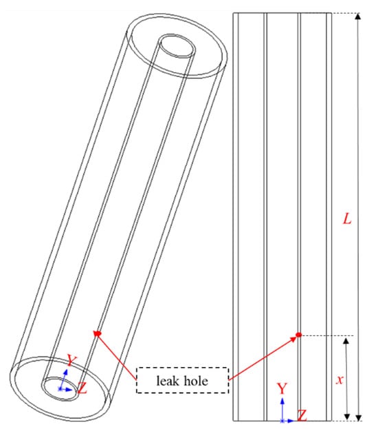
Figure 1.
Oil casing annulus diagram.
The simplified 2D mesh model is shown in Figure 2. The physical model was first constructed and meshed using ICEM, with a model height L = 1 m and a distance x = 0.2 m from the leakage point to the bottom of the model. To enhance mesh quality, triangular mesh elements were selected based on the 2D mesh quality evaluation criteria defined in Equation (8). The grid quality evaluation index [26] for 2D grids is as follows:
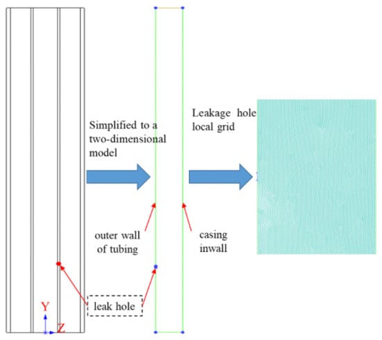
Figure 2.
Two-dimensional grid model.
3D grids:
The three-dimensional (3D) mesh model is illustrated in Figure 3, with a model height L = 1 m and a distance x = 0.2 m from the leakage point to the model’s bottom. Since the focus of this study is the annular space between the tubing and casing, the fluid region inside the tubing is excluded from the model, thereby reducing the total mesh count with equivalent settings and improving computational efficiency. To enhance mesh quality, tetrahedral mesh elements were selected based on the 3D mesh quality evaluation criteria defined in Equation (9). The value of C is shown in Table 2.
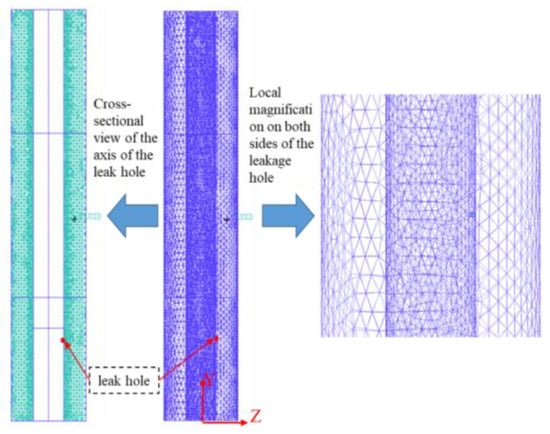
Figure 3.
Three-dimensional grid model.
Table 2.
C values corresponding to different grid types.
After importing the mesh file into Fluent, boundary conditions for the computational model were configured:
- The leakage orifice was set as a velocity inlet, assuming gas from the tubing enters the annulus through the leak at a specified velocity.
- The model’s upper boundary was defined as a pressure-outlet.
- Solid boundaries were assigned as no-slip walls.
The SST k-omega (k-ω) turbulence model was selected for its ability to account for gas compressibility and turbulent shear stresses, ensuring higher computational accuracy and reliability. As analyzed in Section 2.1, the Mixture multiphase flow model was adopted. The Coupled solver was employed, with residual curves iterated to convergence criteria.
With these settings—leakage aperture D = 4 mm, inlet velocity 100 m/s, and outlet pressure 0.1 MPa—both 2D and 3D models simulated gas-phase distributions over a 2 s duration, as shown in Figure 4. The results indicate that gas jets entering the annular liquid generate abundant bubbles under buoyancy, gravity, and turbulent shear forces. These bubbles rise while undergoing fragmentation and coalescence, consistent with general high-speed gas–liquid interaction dynamics. However, the 2D model predicts an unrealistic liquid level rise due to gas intrusion, contrasting sharply with actual annular behavior. In reality, high-velocity gas leaks from the tubing jets perpendicularly into the annulus protection fluid, producing bubbles that ascend while perturbing surrounding liquid. These bubbles traverse the liquid phase, driving intense surface fluctuations that radially disperse under gravity conditions without significant bulk liquid elevation. Since the integrated acoustic model derives sound fields analogously from flow fields, inaccuracies in flow simulations directly compromise acoustic credibility. Given the 2D model’s failure to capture the annular geometry’s structural specificity, this study adopted the 3D physical model.
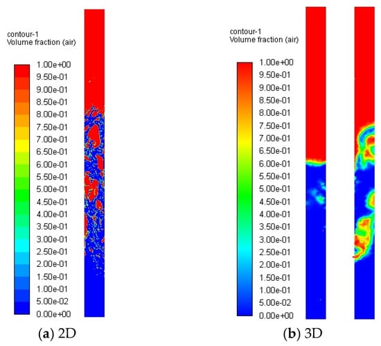
Figure 4.
Gas phase distribution diagram.
3.2. Grid Independence Verification
Fluid dynamics simulation analysis based on Fluent requires not only convergent solutions but also the verification of mesh independence—two fundamental criteria for numerical validity [26,27,28]. Generally, increased mesh density (i.e., smaller element sizes) improves computational accuracy. However, excessive mesh quantities disproportionately reduce computational efficiency, as accuracy gains diminish beyond a critical threshold. To balance precision and practicality, convergent solutions were evaluated across varying mesh resolutions in this study and an optimal mesh configuration was selected for subsequent tubing leakage simulations under diverse operational conditions. Three computational models were designed with mesh counts of 183,000, 370,000, and 560,000 elements, respectively. Simulation parameters are summarized in Table 3.
Table 3.
Simulation parameters.
Figure 5 illustrates gas distribution patterns in the annulus across different mesh densities. The results demonstrate consistent gas jet trajectories and phase dispersion regardless of mesh resolution. To focus on the acoustic field distribution within the annulus following tubing leakage, a series of monitoring points were strategically placed to capture acoustic characteristics. The locations of these monitoring points are shown in Figure 6, with coordinates detailed in Table 4.
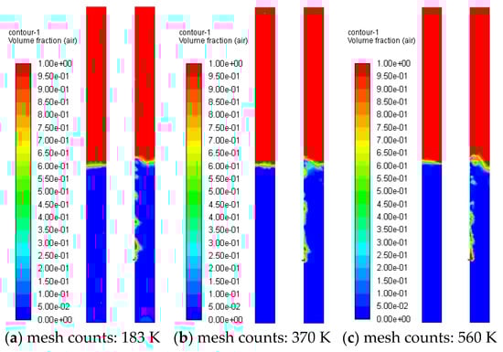
Figure 5.
Distribution of gas in annulus with different numbers of grids.
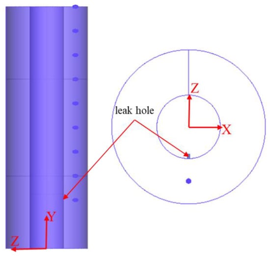
Figure 6.
Schematic diagram of monitoring point setting.
Table 4.
Coordinates of monitoring points.
Figure 7 shows the distribution of the total sound pressure level (SPL) along the Y-axis within the annulus for different mesh densities. The results indicate that higher mesh counts correlate with increased SPL values at the same monitoring points. However, when the mesh count is doubled from 183,000 to 370,000 and tripled to 560,000, the incremental gain in the SPL diminishes significantly, with only minor increases observed. Additionally, the converged solutions from all three mesh configurations exhibit identical trends along the Y-axis, demonstrating qualitative reliability in simulating the acoustic field distribution during tubing leakage. Therefore, under the premise of solution credibility, the 183,000-element mesh model was selected to optimize computational efficiency. The corresponding meshing parameters are listed in Table 5.
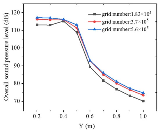
Figure 7.
Effect of grid number on total sound pressure level along the Y-axis.
Table 5.
Meshing parameters.
3.3. The Influence of the Leakage Rate on Annular Flow Field and Sound Field
Using the mesh model from Figure 5a with a leakage aperture D = 4 mm, liquid level depth of 0.5 m, and pressure outlet boundary set to 0.1 MPa, gas distribution patterns in the annulus at varying leakage velocities (10 m/s, 30 m/s, 50 m/s, 100 m/s, and 150 m/s) are illustrated in Figure 8. The results reveal the following:
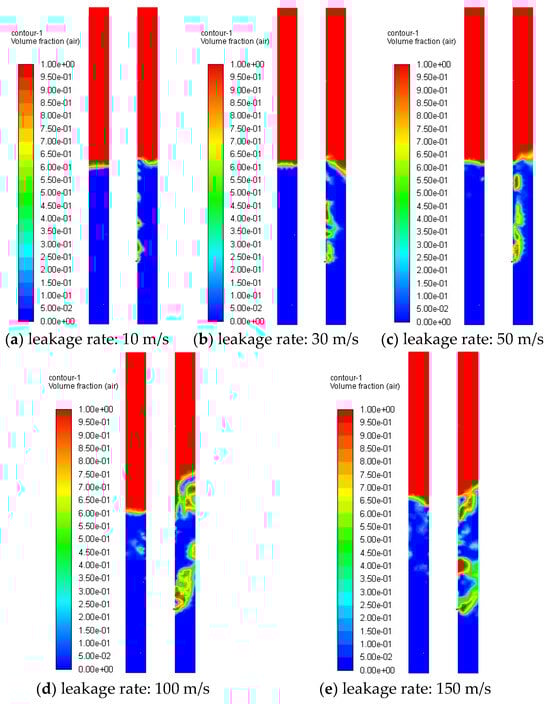
Figure 8.
Distribution of gas in annulus at different leakage rates.
- At low leakage velocities, gas ascends along the tubing wall post-leakage. Acoustic emissions primarily originate from quadrupole sources (generated by fluid interaction forces) and bubble rupture noise as bubbles reach the liquid surface.
- At higher leakage velocities, gas exhibits increased horizontal displacement, impacting the casing inner wall to produce impact noise and generating dipole sources through reverse flow interactions [29].
The velocity distribution of the fluid in the annulus at different leakage rates is shown in Figure 9. As can be seen from the figure, the maximum movement velocity of the gas necessarily occurs immediately before it detaches from the leakage orifice. After the gas detaches from the leakage orifice and is ejected into the liquid, it generates numerous bubbles under the effect of turbulent shear forces. The horizontal velocity rapidly decays, and subsequently, the gas diffuses upward under buoyancy forces. This phenomenon also demonstrates that the primary energy component of leakage noise originates from quadrupole sound sources.
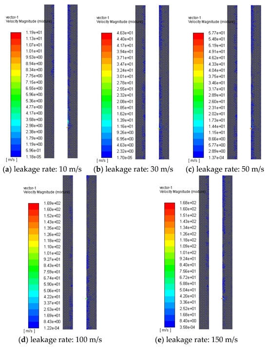
Figure 9.
Velocity distribution of annulus fluid at different leakage rates.
The distribution of total sound pressure level along the Y-axis in the annulus at different leakage rates is shown in Figure 10. As can be observed from the figure, higher leakage rates correspond to greater total sound pressure levels at the same monitoring points, with all values exhibiting gradual attenuation along the Y-axis direction. At the Y = 0.5 m monitoring point, the total sound pressure level of leakage noise plummets abruptly, followed by stabilized attenuation. This phenomenon can be attributed to the positioning of the Y = 0.5 m monitoring point at the gas–liquid interface, where the significant acoustic impedance mismatch between gas and liquid phases causes rapid attenuation of underwater noise transmission through the interface.
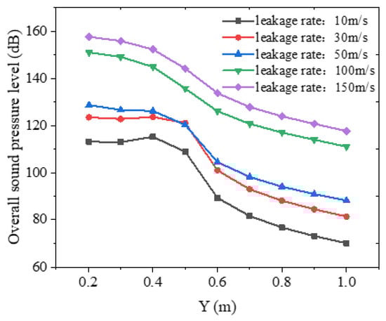
Figure 10.
Distribution of total sound pressure level along Y-axis at different leakage rates.
The time-domain and frequency-domain characteristics of leakage noise at the identical monitoring point (coordinates (0, 0.9, −0.076)) at different leakage rates are presented in Figure 11 and Figure 12, with the sound pressure at time zero measuring 9.1 × 10⁴ Pa. As shown in the figures, the leakage noise exhibits consistent variation trends in both temporal and spectral domains, where the sound pressure values at identical frequencies demonstrate an increasing trend with higher leakage rates. Notably, distinct impulsive tones observed in the time-domain profiles correspond to shock signals generated by bubble collapse upon reaching the liquid surface.
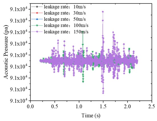
Figure 11.
Time domain curve of noise at the same monitoring point at different leakage rates.
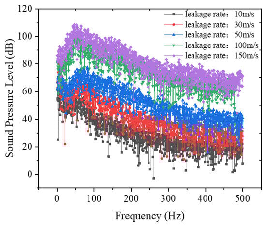
Figure 12.
Frequency distribution of noise at the same monitoring point at different leakage rates.
The boundary conditions applied in Figure 8, Figure 9, Figure 10, Figure 11 and Figure 12 utilize pressure-outlet settings, with computational simulation results demonstrating near-field noise distribution patterns adjacent to leakage points at both ends of the annulus. In actual well completion configurations, the annular space is capped by a tubing hanger at its upper terminus, forming a confined volume with annular protection fluid. This indicates that gas leakage into the annulus constitutes a pressure-accumulation process, where acoustic waves undergo multiple reflections between the tubing hanger and the annular fluid interface. Consequently, acoustic signals detected by sensors at the annular outlet represent superimposed reflections. Therefore, it is essential to model the annulus as a confined system with reflective boundary conditions at its upper boundary to characterize full-scale acoustic wave propagation. Adopting the mesh configuration shown in Figure 5 a with a liquid column depth fixed at 0.5 m, leakage velocities were parametrically set to 10 m/s, 30 m/s, 50 m/s, 100 m/s, and 150 m/s while implementing no-slip wall boundary conditions at the model’s upper boundary.
Figure 13 demonstrates gas distribution patterns within the confined annulus at varying leakage rates. Comparative analysis with Figure 8 reveals that annular confinement exerts minimal influence on gas migration dynamics in the liquid phase. The dominant transport mechanisms remain governed by buoyancy effects and turbulent shear forces, signifying that leakage rates primarily modulate quadrupole source components in leakage noise spectra while exhibiting negligible impact on bubble collapse acoustics post interface breakthrough.
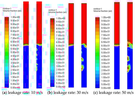
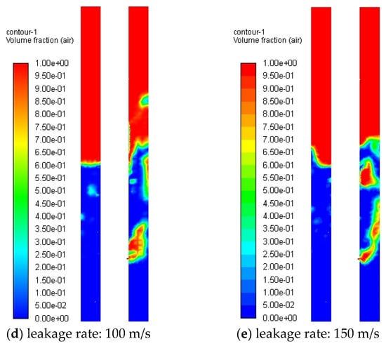
Figure 13.
Gas distribution in annulus at different leakage rates (WALL).
Figure 14 illustrates the distribution of the total sound pressure level along the Y-axis at different leakage rates when the annular space is enclosed. A comparison with Figure 10 reveals that under the same leakage conditions, the total sound pressure level of the leakage noise significantly increases in the enclosed annular space, and the attenuation rate along the Y-axis direction is markedly reduced. This is attributed to the multiple reflections and superposition of leakage noise within the enclosed annular space. It also indicates that, compared to an open diffusion field, the enclosed annular structure extends the propagation distance of the leakage acoustic waves. Figure 15 displays the frequency distribution curves of the leakage noise at different leakage rates in the enclosed annular space, conforming to the general trend of aerodynamic noise energy decreasing with increasing frequency: the sound level of the leakage noise diminishes as the frequency rises.
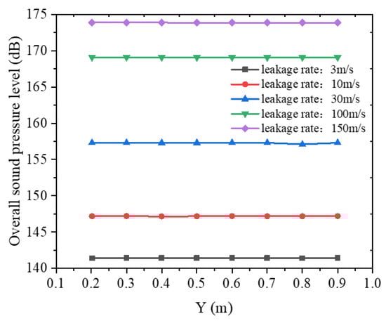
Figure 14.
Distribution of total sound pressure level along the Y-axis at different leakage rates (WALL).
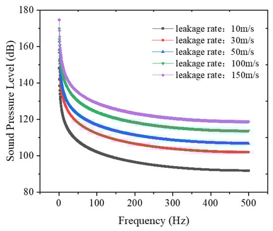
Figure 15.
Frequency domain distribution curve of leakage noise at different leakage rates.
3.4. The Influence of Leakage Aperture on Annular Flow Field and Sound Field
Utilizing the mesh configuration referenced from Figure 5a with a fixed leakage velocity of 10 m/s and pressure-outlet boundary conditions at the upper boundary, numerical simulations were conducted for leakage orifice diameters of 4 mm, 6 mm, 8 mm, 10 mm, and 12 mm. Figure 16 displays the gas distribution patterns within the annulus across varying orifice dimensions, while Figure 17 presents Y-axis profiles of the total sound pressure level (SPL), demonstrating a positive correlation between the leakage orifice diameter and SPL magnitude under constant flow velocity conditions. Figure 18 further characterizes the frequency-domain distributions of leakage noise, revealing spectral variations induced by geometric modifications of leakage ports.
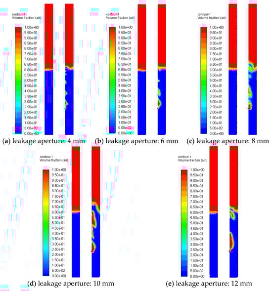
Figure 16.
Gas distribution in annulus for different leakage apertures.
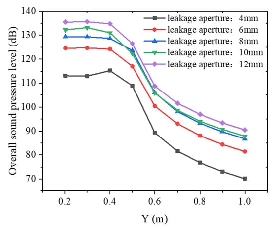
Figure 17.
Distribution of total sound pressure level along the Y-axis for different leakage apertures.
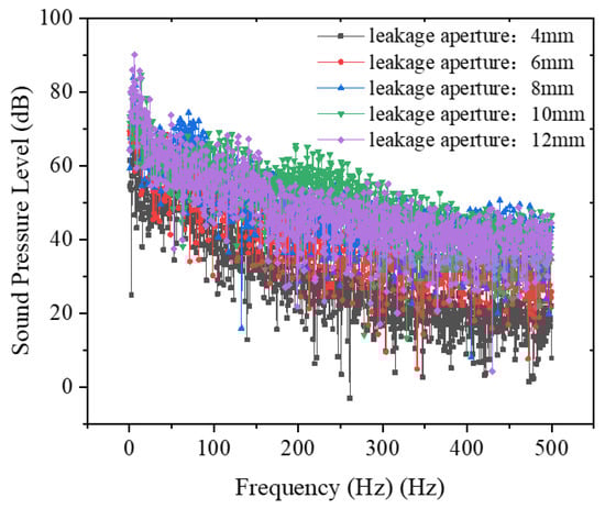
Figure 18.
Frequency domain distribution curve of leakage noise for different leakage apertures.
3.5. The Influence of Liquid Level Depth on Annular Flow Field and Sound Field
Adopting the mesh parameters from Figure 5a with vertical scale extended to 2 m, numerical simulations were performed under controlled conditions: a fixed leakage velocity of 10 m/s, orifice diameter D = 8 mm, and no-slip wall boundary implementation at the upper boundary. This parametric study systematically examined liquid column depths spanning 0.5 m, 0.8 m, 1.0 m, 1.2 m, and 1.5 m to characterize annular fluid–gas interaction dynamics under geometric scaling conditions.
Figure 19 demonstrates gas dispersion characteristics within the annulus for varying liquid column depths, revealing enhanced gas–liquid interfacial interactions during buoyancy-driven ascent with increasing depth. Figure 20 delineates corresponding Y-axis profiles of the total sound pressure level (SPL), establishing a direct correlation between reduced gas-phase volume fraction (from 38% to 12% as liquid level elevates) and amplified SPL measurements at equivalent monitoring positions. Figure 21 further quantifies frequency-dependent acoustic energy distributions, showing 6–15 dB/Hz increases in spectral energy density across 100–1000 Hz bands per 0.3 m liquid level increment, indicative of acoustic energy redistribution phenomena in constrained annular geometries.
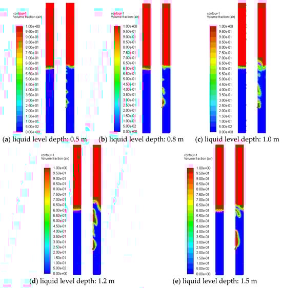
Figure 19.
Gas distribution in annulus at different liquid level depths.
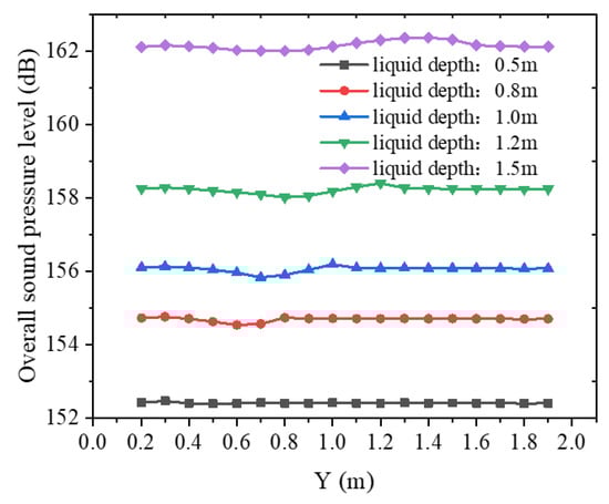
Figure 20.
Distribution of total sound pressure level along the Y-axis at different liquid level depths.
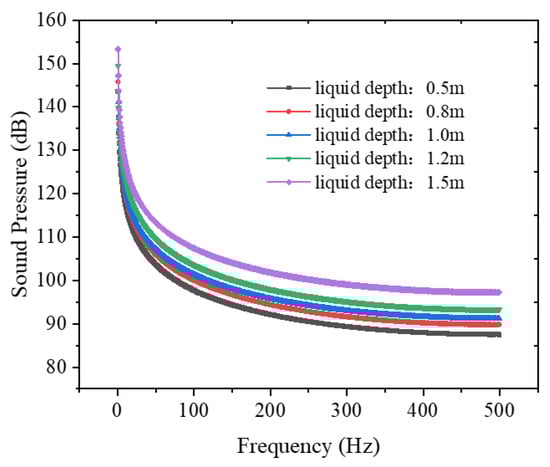
Figure 21.
Frequency distribution curve of leakage noise at different liquid level depths.
3.6. Comparative Analysis of Leakage Above and Below the Liquid Level
Utilizing the mesh configuration from Figure 19c with fixed parameters (leakage velocity = 10 m/s, orifice diameter D = 8 mm, no-slip wall boundary), numerical simulations were conducted for liquid column depths of 0 m and 1.0 m. Figure 22 compares annular flow field distributions between above-liquid-level and submerged leakage scenarios. In gas-phase leakage (liquid level = 0 m), tubing gas jets directly impact the casing wall, generating acoustic components comprising (1) monopole sources from wall impingement, (2) dipole sources from reversed flow interactions, and (3) quadrupole sources from fluid turbulence. Quadrupole sources dominate the acoustic energy spectrum, while monopole components exhibit minimal energy contributions. Figure 23 illustrates the Y-axis distribution profiles of the total sound pressure level (SPL) for leakage noise, demonstrating that submerged leakage conditions yield higher SPL values at equivalent monitoring positions compared to above-liquid-level leakage scenarios. Figure 24 demonstrates frequency-domain consistency where spectral decay characteristics remain congruent across both leakage configurations.
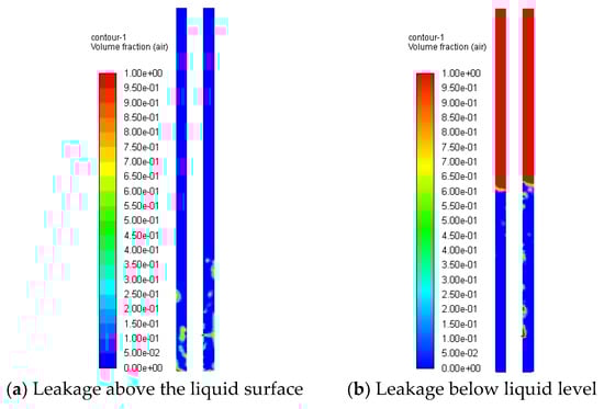
Figure 22.
Flow field distribution of leakage annulus above and below liquid level (WALL).
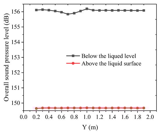
Figure 23.
Distribution of total sound pressure level of leakage along the Y-axis above and below liquid level.
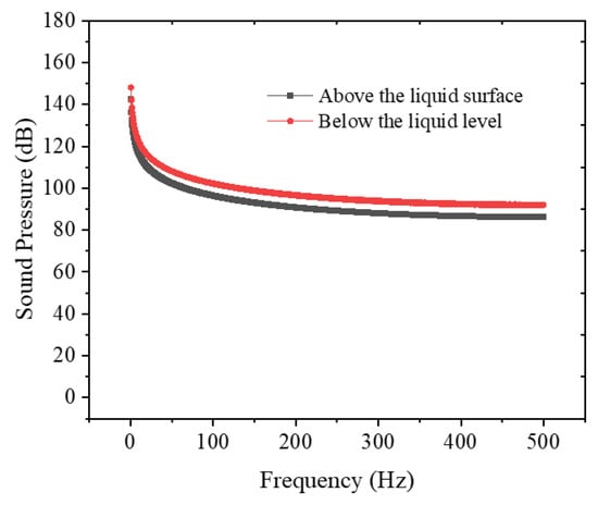
Figure 24.
Frequency distribution curve of leakage noise above and below liquid level.
3.7. The Influence of the Number of Leakage Points on the Annular Flow Field and Sound Field
Utilizing the mesh configuration from Figure 19c, numerical simulations were conducted for multi-point leakage scenarios (one, two, and three leakage points) with fixed parameters: leakage velocity = 10 m/s, orifice diameter D = 8 mm, liquid column depth = 1.0 m, and no-slip wall boundary conditions. Figure 25 and Figure 26 depict gas dispersion patterns for different leakage point configurations, demonstrating that liquid-phase interactions significantly influence gas jet motion trajectories—this hydrodynamic interaction constitutes the primary mechanism driving source composition variations in leakage noise.
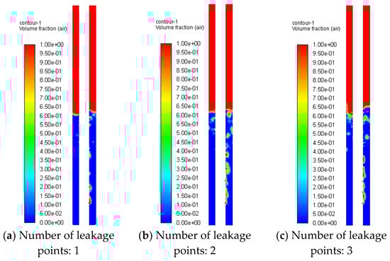
Figure 25.
Gas distribution in annulus with different numbers of leakage points (below liquid level).
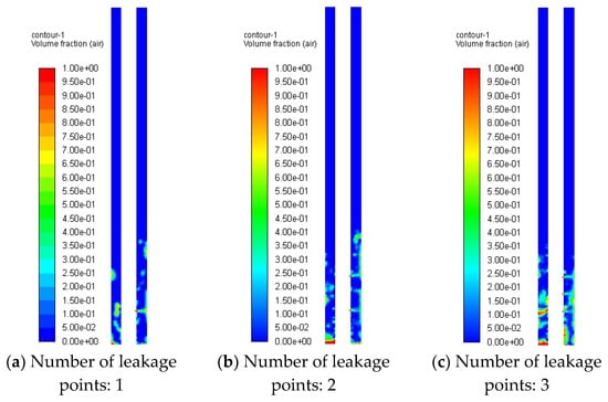
Figure 26.
Gas distribution in annulus for different numbers of leakage (above liquid level).
Figure 27 and Figure 28 present Y-axis distribution profiles of the total sound pressure level (SPL) for varying leakage point quantities, demonstrating that SPL values at identical monitoring positions increase with the number of leakage points while exhibiting a non-linear relationship with point multiplicity. Figure 29 and Figure 30 show frequency-domain characteristics of leakage noise across different point configurations, revealing that leakage point density primarily modulates the spectral energy content without altering the fundamental frequency distribution characteristics.
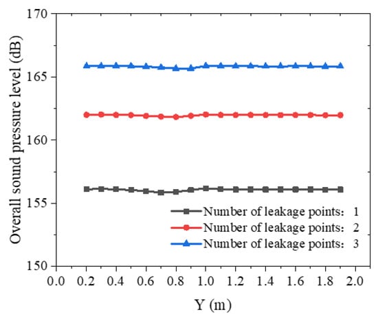
Figure 27.
Distribution of total sound pressure level along the Y-axis for different numbers of leakage points (below liquid level).
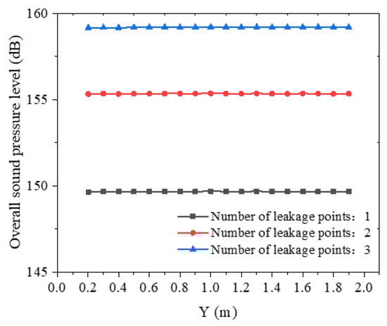
Figure 28.
Distribution of total sound pressure level along the Y-axis for different numbers of leakage points (above liquid level).
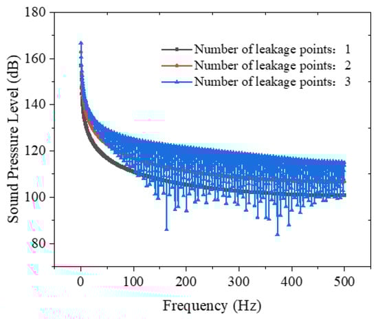
Figure 29.
Frequency distribution curves of leakage noise for different numbers of leakage points (below liquid level).
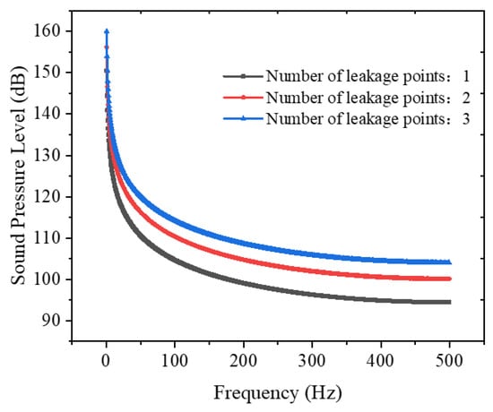
Figure 30.
Frequency distribution curves of leakage noise for different numbers of leakage points (above liquid level).
4. Conclusions
Through numerical simulations of annular flow fields and acoustic fields in various downhole tubing leakage scenarios, the following conclusions are drawn:
- (1)
- The leakage rate, orifice diameter, and number of leakage points are primary factors affecting leakage noise energy levels. The total sound pressure level of leakage noise increases with higher leakage rates, larger orifice diameters, and greater numbers of leakage points.
- (2)
- The frequency-response curves of downhole tubing leakage noise in gas wells align with general principles of aerodynamic noise: Leakage noise amplitude decreases with increasing frequency. At varying leakage rates, orifice diameters, and leakage point quantities, leakage noise consistently exhibits broadband characteristics with identical variation trends.
- (3)
- When leakage occurs below the liquid level, the generated aerodynamic noise can propagate upward through the annular gas column by penetrating the liquid phase. Due to significant acoustic impedance mismatch between gas and liquid phases, noise originating below the liquid level undergoes substantial attenuation when traversing the gas–liquid interface.
- (4)
- The confined annular structure enables the repeated reflection and superposition of leakage noise within the annular space, thereby extending the propagation distance of leakage-induced acoustic waves.
- (5)
- This study is confined to investigating the feasibility of detecting tubing leakage below annular fluid at the wellhead using acoustic methods. It did not extend to determining optimal detection modalities or analytical methodologies, which should be explored in future research.
Author Contributions
Conceptualization, Y.-P.Y.; methodology, B.-C.S.; software, Y.-P.Y. and M.-S.L.; validation, Y.-H.J. and J.-Y.W.; formal analysis, Y.-P.Y.; investigation, Y.-P.Y. and B.-C.S.; resources, J.-C.F.; data curation, M.-S.L.; writing—original draft preparation, Y.-P.Y.; writing—review and editing, Y.-F.G.; visualization, S.L.; supervision, Y.-S.Z.; project administration, J.-Y.W.; funding acquisition, J.-Y.W. All authors have read and agreed to the published version of the manuscript.
Funding
This research was funded by “EVOLUTION MECHANISM OF MAJOR RISKS IN COMPLEX OIL AND GAS DRILLING AND PRODUCTION AND INTELLIGENT SAFETY OPERATION AND MAINTENANCE METHODS” and “RESEARCH AND APPLICATION OF QUALITY, SAFETY, AND ENVIRONMENTAL RISK CONTROL TECHNOLOGIES FOR OIL AND GAS FIELDS”, grant number “2023 DJ6508” and “2024 YQX20102”.
Data Availability Statement
All data generated or analyzed during this study are included in this published article.
Conflicts of Interest
Authors Yun-Peng Yang, Bing-Cai Sun, Ying-Hua Jing, Jin-You Wang, Yi-Fan Gan, Shuang Liang, Yu-Shan Zheng and Mo-Song Li were employed by the CNPC Research Institute of Safety & Environment Technology. Author Jian-Chun Fan was employed by the China University of Petroleum.
Abbreviations
The following abbreviations are used in this manuscript:
| VOF | Volume of Fluid |
| CAA | Computational aeroacoustics |
| FW-H | Ffowcs Williams–Hawkings |
| N-S | Navier–Stokes |
| SPL | Sound pressure level |
| 2D | Two-dimensional |
| 3D | Three-dimensional |
| ID | Inner diameter |
| OD | Outer diameter |
| ICEM | The Integrated Computer Engineering and Manufacturing Code |
References
- Wang, Y.B.; Zeng, J.; Gao, D.L. Effect of annular pressure on the fatigue damage of deepwater subsea well-heads. Nat. Gas Ind. 2020, 40, 116–123. [Google Scholar]
- Zhang, B.; Luo, F.W.; Sun, B.; Xie, J.; Xu, Z.; Liao, H. A method for wellbore integrity detection in deep oil and gas wells. Pet. Drill. Tech. 2021, 49, 114–120. [Google Scholar]
- Li, Q.; Cao, Y.F.; Lu, S.J.; OuYang, T.B.; Yang, X.Q.; He, B.S.; Zhou, J.L.; Li, Y.B.; Fan, Z.L.; Wu, Z.Q. Well integrity status and solutions of offshore oil and gas wells. Offshore Oil Gas 2018, 30, 115–122. [Google Scholar]
- Yang, Y.P.; Fan, J.C.; Lu, S.J. Technology and engineering practice of detection and plugging of down-hole oil casing leakage in offshore gas wells. China Offshore Oil Gas 2021, 33, 145–150. [Google Scholar]
- Li, Q.; Li, Q.; Han, Y. A Numerical Investigation on Kick Control with the Displacement Kill Method during a Well Test in a Deep-Water Gas Reservoir: A Case Study. Processes 2024, 12, 2090. [Google Scholar] [CrossRef]
- Bateman, R.M. Cased-Hole Log Analysis and Reservoir Performance Monitoring, 2nd ed.; Springer: Berlin/Heidelberg, Germany, 2015. [Google Scholar]
- Johns, J.E.; Blount, C.G.; Dethlefs, J.C.; Julian, J.Y.; Loveland, M.J.; McConnell, M.L.; Schwartz, G.L. Applied ultrasonic technology in wellbore-leak detection and case histories in Alaska North Slope wells. SPE Prod. Oper. 2009, 24, 225–232. [Google Scholar] [CrossRef]
- Vogtsberger, D.C.; Girrell, B.; Miller, J.; Spencer, D. Development of High-Resolution axial flux leakage casing-inspection tools. In Proceedings of the SPE Eastern Regional Meeting, Morgantown, WV, USA, 14–16 September 2005. SPE 97807-MS. [Google Scholar]
- Cao, Z.; Hu, B.; Li, Z.; Zhang, J. Research status of acoustic wave identification and location methods for gas pipeline leakage. Nondestruct. Test. 2023, 45, 49–57. [Google Scholar]
- Liu, D.; Fan, J.C.; Wu, S.N. Acoustic wave-based method of locating tubing leakage for offshore gas wells. Energies 2018, 11, 3454. [Google Scholar] [CrossRef]
- Yang, Y.; Fan, J.; Wu, S.; Liu, D.; Ma, F. Multi-acoustic-wave-feature-based method for detection and quantification of downhole tubing leakage. J. Nat. Sci. Eng. 2022, 102, 104582. [Google Scholar] [CrossRef]
- Liu, C.W. Leak-Acoustics Generation and Propagation Characteristics for Natural Gas Pipelines. Ph.D. Thesis, University of Petroleum, Qingdao, China, 2016. [Google Scholar]
- Yan, C.W.; Han, B.K.; Bao, H.Q. Research on acoustic source characteristics of gas pipeline leakage. Tech. Acoust. 2017, 36, 110–115. [Google Scholar]
- Lyu, N.Y.; Fan, J.C.; Liu, D.; Liu, S.J.; Wen, M.; Liang, Z.W. Simulation study on leakage acoustic source characteristics of gas wel tubing and casing. China Pet. Mach. 2017, 45, 79–82. [Google Scholar]
- Zheng, L.; CAX Technology Alliance. ANSYS Fluent 15.0 Fluid Calculation from Beginner to Expert, Upgraded ed.; Electronic Industry Press: Beijing, China, 2015. [Google Scholar]
- Xu, J. A Comprehensive Self-Study Guide to ANSYS Workbench 15.0; Electronic Industry Press: Beijing, China, 2014. [Google Scholar]
- Fan, J.; Peng, H. Advanced Applications of Fluent and Case Analysis; Tsinghua University Press: Beijing, China, 2008. [Google Scholar]
- Ye, M.; Yan, G.; Scheuermann, A. Discrete bubble flow in granular porous media via multiphase computational fluid dynamic simulation. Front. Earth Sci. 2022, 10, 947625. [Google Scholar]
- Zheng, J. Application of a Broadband Sound Source Model Based on Proudman’s Theory in the Prediction of Automobile Aerodynamic Noise Sources. J. Sichuan Ordnance Ind. 2011, 32, 54–57. [Google Scholar]
- Wang, C.; Xing, H.; Zheng, J. Simulation Study on Aerodynamic Noise of High-Speed Train Based on CAA. J. East China Jiaotong Univ. 2015, 32, 7. [Google Scholar]
- Si, H.Q.; Shi, T.; Shen, W.Z.; Wu, X.J. Advanced Time Methods for Noise Prediction of FW-H Equation. J. Nanjing Univ. Aeronaut. Astronaut. 2013, 45, 6. [Google Scholar]
- Rodrigues, S.S.; Marta, A. On addressing noise constraints in the design of wind turbine blades. Struct. Multidiscip. Optim. 2014, 50, 489–503. [Google Scholar] [CrossRef]
- Huang, Y.M.; Chen, T.C.; Shieh, P.S. Analytical Estimation of the Noise Due to a Rotating Shaft. Appl. Acoust. 2014, 76, 187–196. [Google Scholar] [CrossRef]
- Li, W.; Zhang, Y.J.; Long, F.F.; Liu, Y.J. Acoustic Detection Method and Experimental Research on Inner Tube Leakage in Jacketed Structure. Chem. Mach. 2017, 44, 145–148. [Google Scholar]
- Zhang, H.; Yuan, G.; Li, G.; Li, J.; Wan, J.; Fu, P. Numerical Simulation Research on the Leakage Flow Field of Gas Well Tubing and Casing. Pet. Mach. 2020, 12, 48. [Google Scholar]
- Yang, L.; Yang, F.S. Verification of Grid Independence for Bent Square Tubes Based on FLUENT. J. Beibu Gulf Univ. 2023, 38, 63–69. [Google Scholar]
- Yan, W.; Wang, D.; Hu, Q.; Zhou, Y.J.; Zheng, X.Q. Grid Independence Analysis of Gas Membrane Seal Based on CFD in T-shaped Groove. Lubr. Seal. 2018, 43. [Google Scholar]
- Xie, Y.; Ren, J.B.; Huang, H.H.; Zhang, X. Analysis of Computational Fluid Dynamics Grid Independence Based on Chi-Square Test. Sci. Eng. Technol. 2020, 20, 123–127. [Google Scholar]
- Zhang, Q. Fundamentals of Aeroacoustics; National Defense Industry Press: Beijing, China, 2012. [Google Scholar]
Disclaimer/Publisher’s Note: The statements, opinions and data contained in all publications are solely those of the individual author(s) and contributor(s) and not of MDPI and/or the editor(s). MDPI and/or the editor(s) disclaim responsibility for any injury to people or property resulting from any ideas, methods, instructions or products referred to in the content. |
© 2025 by the authors. Licensee MDPI, Basel, Switzerland. This article is an open access article distributed under the terms and conditions of the Creative Commons Attribution (CC BY) license (https://creativecommons.org/licenses/by/4.0/).