Numerical Analysis of Pipe–Soil Interaction Using Smoothed Particle Hydrodynamics (SPH)

Abstract

Pipe–soil interaction encompasses the study of stress distributions and deformation mechanisms occurring between buried pipelines and their surrounding soil. Understanding the mechanical behavior of this coupled system is essential for the analysis of deformation patterns and failure modes in buried pipelines, thereby providing critical guidance for construction design and risk assessment protocols. Traditional analytical approaches have relied on classical mechanics theories and experimental methodologies; however, these approaches often incorporate excessive simplifications and assumptions that inadequately represent the complex properties of both soil and pipeline structures. Numerical simulation methodologies have emerged as viable alternatives for investigating pipe–soil interaction. Among these numerical approaches, Smoothed Particle Hydrodynamics (SPH)—an advanced Lagrangian meshless particle method—offers distinct advantages in modeling complex behaviors, including free surfaces, deformable boundaries, and large deformation scenarios that characterize pipe–soil interaction. This research establishes a pipe–soil interaction model for buried pipelines utilizing the SPH method, incorporating elastic–plastic constitutive relationships to represent soil behavior. The investigation examines lateral interaction mechanisms, vertical interaction responses in sandy soils, and the parametric influence of various soil properties on pipe–soil interaction characteristics. This study contributes insights into the application of meshfree numerical simulation techniques for pipe–soil interaction analysis, offering both engineering utility and theoretical advancement for pipeline infrastructure design and safety assessment.

1. Introduction

Pipelines serve as key transportation infrastructure that plays a crucial role in maintaining resource distribution networks, ensuring energy security, and supporting modern living standards by efficiently moving essential resources like water, natural gas, and petroleum products. Buried pipelines exist in complex physical environments where the surrounding soil both constrains them and transmits various forces to them. Research and failure analyses show that pipeline problems mainly arise from soil–pipe interactions under different ground and environmental conditions. Therefore, understanding how buried pipelines and soil interact mechanically is essential for accurately describing how pipelines deform, predicting how they might fail, creating reliable risk assessment methods, and improving engineering design for better structural strength and longer operational life. Standard experiments studying pipe–soil interactions face significant challenges because soil is naturally complex and varied in composition. The relationship between buried pipelines and surrounding soil involves many interactions over long time periods, with outcomes affected by factors such as how deep the pipe is buried, the pipe’s diameter, soil friction properties, and other ground-related factors that vary by location and time. Traditional theories and testing methods not only require substantial resources and time but also have limitations in capturing the full interaction processes and predicting how systems respond to complex forces, making it harder to develop complete predictive models.

Recent advances in computing technologies and numerical algorithms have enabled the development of advanced simulation methods as effective alternatives for studying buried pipe–soil interaction. These computational approaches offer essential insights into underlying physical processes that would be difficult to access through conventional experiments, improving predictive ability and design optimization for buried pipeline systems. Among current numerical methods, the finite element method (FEM) has become the popular analytical technique for investigating pipe–soil interactions, widely used in geotechnical and pipeline engineering fields. FEM offers unique advantages in simulating coupled soil–pipeline systems through its ability to incorporate complex material models, interface elements, and boundary conditions while enabling thorough residual strength assessments critical for pipeline integrity evaluation and service life prediction [1,2]. The analytical framework provided by FEM allows detailed characterization of complex relationships between key mechanical response indicators (including maximum radial compressive stress distributions, principal stress orientations, and maximum shear stress concentrations) and fundamental influencing factors such as burial depth, soil cohesion properties across various moisture conditions, internal friction angle variations, and pipe–soil interface friction coefficients under different loading conditions [3,4]. This ability to analyze multiple factors has greatly improved understanding of buried pipeline system behavior and enhanced design optimization methods.

The theoretical framework for understanding buried pipeline–soil interactions has developed considerably through extensive experimental studies and numerical analyses conducted by researchers worldwide. This ongoing development has produced increasingly refined interpretative and predictive models for complex soil–structure interaction. Mahdavi et al. [5] employed a comprehensive composite model approach to investigate these interactions, particularly highlighting the importance of geotechnical loading parameters on pipeline mechanical response characteristics. Their work established key principles for the integrated analysis of soil mechanics and structural pipeline behavior, demonstrating the essential need to consider geotechnical loads in pipeline design protocols. Jung et al. [6,7] made significant contributions to the field through methodical numerical simulations examining shallow-buried pipe–soil lateral interactions, later extending their analytical framework to deeply buried pipeline systems (characterized by depth-to-diameter ratios exceeding 15) embedded in sandy soil matrices. Their research revealed important transition mechanisms between shallow and deep burial response behaviors, including distinct differences in soil failure patterns and ultimate resistance values that had previously been inadequately described in the literature. Through systematic parameter studies, they established quantitative relationships between burial depth ratios and lateral soil resistance coefficients that have become valuable in current pipeline design practice.

Building on these foundational contributions, Dong et al. [8] established velocity-dependent correlations between soil ultimate resistance and pipe displacement rates using a coupled large-deformation finite element model with a modified Cam-Clay constitutive relationship, offering critical insights for dynamic scenarios like seismic events. Roy et al. [9] compared conventional and Modified Mohr–Coulomb (MMC) models in FEM frameworks, demonstrating MMC’s superiority in capturing post-peak strain-softening behavior and emphasizing constitutive model selection’s importance for large-deformation predictions. In the context of geohazard interaction with pipeline infrastructure, Tang et al. [10] quantified how geometric parameters (e.g., diameter-to-thickness ratios, burial depth) mitigate landslide-induced pipeline deformations, providing design guidelines for unstable regions. Addressing pipeline integrity assessment, Wang et al. [11,12] developed a multifactorial leakage risk framework incorporating pressure differentials, burial conditions, and geotechnical properties. This multifactorial analysis established a comprehensive framework for assessing pipeline leakage risks and predicting contaminant transport patterns in surrounding soil. Wang et al. [13] identified through numerical simulations that pipelines under lateral landslide loading exhibit maximum stress concentrations at landslide boundaries and peak deformations in central landslide zones, guiding targeted reinforcement and monitoring strategies for vulnerable sections. Han et al. [14,15] developed parametric models specifically designed to evaluate soil collapse impacts on buried pipeline systems. Their analytical framework incorporated multiple influential variables including soil mechanical properties, collapse geometry characteristics, and pipeline structural parameters to predict resulting stress distributions and deformation patterns under various collapse scenarios, enhancing vulnerability assessments and protective measures for high-risk areas [16,17]. These studies collectively improve predictive capabilities for pipeline behavior under complex loading and geohazard conditions, informing optimized engineering.

Despite the advances in numerical modeling of pipe–soil interaction, important methodological limitations remain in current analytical approaches. The FEM, despite its widespread use and proven capabilities, shows inherent limitations that become problematic in certain simulation scenarios. FEM experiences notable accuracy declines under large deformation conditions or during crack propagation—both commonly encountered in pipeline–soil interaction subjected to ground movement. This is particularly evident in scenarios involving soil liquefaction-induced lateral spreading, where SPH methods have demonstrated superior capability in tracking particle migration and shear band formation without mesh distortion constraints [18,19,20]. The fundamental challenge stems from the mesh-based nature of FEM, where significant element distortion inevitably occurs during substantial soil or structural deformations, requiring frequent remeshing operations that introduce interpolation errors and computational inefficiencies. These mesh distortion issues considerably compromise simulation reliability and prediction accuracy when modeling extreme soil–pipeline displacement events such as those occurring during fault ruptures, liquefaction-induced lateral spreading, or substantial landslide movements. Furthermore, discontinuities such as crack formation and propagation remain difficult to represent within conventional FEM frameworks without implementing specialized techniques. To address these limitations, existing studies have developed various mesh-free numerical frameworks for pipeline–soil interaction analysis. Tang et al. [21] implemented Smoothed Particle Hydrodynamics (SPH) to successfully capture key mechanical response parameters including pipe ovality evolution and stress–strain distributions during excavation-induced damage. This aligns with SPH’s proven capability in modeling water-soil coupling through multilayer particle systems, where Drucker–Prager elastoplastic models for soil phase and incompressible fluid models achieve high-precision pressure distribution predictions [22]. Li et al. [23] conducted a review of the Material Point Method (MPM) in engineering geological interfaces (slip surfaces and seepage interfaces). They proposed a multi-physics coupling framework and simulated soil–structure interactions using a virtual particle model, effectively mitigating boundary penetration issues at contact interfaces. Qin et al. [24] integrated the Discrete Element Method (DEM) with a meshless approach to simulate granular soil–pipeline interactions. In their stability analysis of sandy soil–pipeline systems, DEM was employed to model particle motion, while the meshless method addressed continuum responses. This coupled methodology demonstrated effectiveness in capturing particle migration and shear band formation mechanisms. The SPH-DEM hybrid approach has been further enhanced through dynamic buffer boundary treatments, reducing virtual particle requirements while maintaining numerical stability in large deformation scenarios [25]. Li et al. [26] developed a three-dimensional Element-Free Galerkin (EFG) code to analyze displacement fields and additional stress distributions in foundations under vertical loading. Li et al. [27] extended a two-dimensional Discontinuous Deformation Analysis (DDA) algorithm to model capillary interactions among unsaturated soil particles. By establishing a soil–water characteristic curve model, their work elucidated the influence of soil suction forces on deformation mechanisms in pipeline-surrounding soils. The extension of SPH to two-phase mixture theory has enabled coupled simulation of solid deformation and solute transport in deformable porous media, providing new insights into unsaturated soil–pipeline interaction mechanisms.

Among them, the SPH approach eliminates mesh distortion concerns through its Lagrangian particle discretization methodology, thereby offering superior capabilities in modeling large deformation and crack evolution processes without encountering the numerical instabilities characteristic of mesh-based approaches. This particle-based formulation enables accurate representation of material discontinuities and interfacial behaviors critical to pipeline–soil interaction. In this paper, a developed SPH model is proposed to investigate three aspects of pipe–soil interaction:

• Soil failure and associated load–displacement relationships under lateral interaction conditions across varying depth-to-diameter ratios (covering both shallow and deep burial configurations).
• Parametric analysis of mechanical responses exhibited by buried pipelines embedded in soil characterized by different properties, specifically the influence of varying cohesion values and internal friction angle characteristics.
• Vertical interaction between pipelines and surrounding soil, with particular emphasis on uplift and settlement response characteristics under controlled displacement.格

Through these investigations, the present study aims to demonstrate SPH methodology’s effectiveness in overcoming traditional mesh-based limitations while providing new insights into fundamental pipeline–soil interaction.

2. Pipe-Soil Interaction Model

2.1. The Basics of SPH Method

The Smoothed Particle Hydrodynamics (SPH) method constitutes a fundamentally Lagrangian interpolation approach characterized by two principal computational steps: kernel approximation of field functions and systematic particle discretization [28]. This methodology effectuates the transformation of continuous integral representations into discrete particle approximations, as mathematically formulated in Equation (1). Within the SPH framework, the physical system is represented through a collection of particles, each possessing individual attributes including mass, density, pressure, and velocity while occupying distinct spatial domains. Each computational particle interacts with neighboring particles situated within a defined smoothing length through kernel functions, with these interactions governed by fundamental conservation laws and appropriate constitutive relationships.

This particle-based computational framework inherently eliminates the mesh constraints characteristic of conventional numerical methods, thereby enabling robust modeling of complex mechanical phenomena including large deformations, material fracture processes, and multiphase interactions in pipeline–soil systems. The absence of fixed connectivity between particles provides advantages when simulating discontinuous phenomena such as soil failure surfaces and interface behavior, which present considerable challenges for mesh-based methodologies. Additionally, the Lagrangian nature of SPH facilitates intuitive tracking of material histories and interfaces, particularly valuable for characterizing evolving contact conditions between pipelines and surrounding soil.

$$〈f(x)〉={\displaystyle \underset{\Omega }{\int }f}(x^{\prime })W(x-x^{\prime },h)\mathrm{d}{x}^{\prime }={\displaystyle {\sum }_{j=1}^N\frac{m_j}{{\rho }_j}}f(x_j)W_{ij}$$

(1)

where $N$ is the number of physical particles; $j$ is the index of particles within the support domain of particle $i$; $m_j$ is the mass of particle j, $m_j=\Delta V_j{\rho }_j$; ${\rho }_j$ is the density of particle j.

The smoothing kernel function $W(x-x^{\prime },h)$ in SPH, also known as the interpolation kernel function, determines the range of a particle’s support domain. Here, h is the smoothing length of the kernel function. When h→0, the kernel function approximates the Dirac delta function $\delta$. The selection of the kernel function governs the consistency and accuracy of the kernel approximation and particle approximation. This study employs the cubic spline kernel function [29], as shown in Equation (2)

$$W(R,h)={\alpha }_d\left\{\begin{array}{ll}{\displaystyle \frac{2}{3}}-R^2+{\displaystyle \frac{1}{2}}{R}^3,& 0\le R<1;\\ {\displaystyle \frac{1}{6}}{(2-R)}^3,& 1\le R<2;\\ 0,& R\ge 2\end{array}\right.$$

(2)

where $R$ represents the relative distance between two particles at points $x$ and $x^{\prime }$, defined as $R=\left|x-x\prime \right|/h$;

${\alpha }_d$ is $1/h$, $15/7\pi h^2$, and $3/2\pi h^3$ in one-, two- and three-dimensional space, respectively.

By discretizing the fundamental conservation equation and momentum conservation laws of continuum mechanics, the SPH-discretized governing equations are derived, as shown in Equations (3) and (4).

$${\displaystyle \frac{d{\rho }_i}{dt}}={\displaystyle {\sum }_{j=1}^N{m}_j}(v_i^{\alpha }-v_j^{\alpha }){\displaystyle \frac{\partial W_{ij}}{\partial x_i^{\alpha }}}$$

(3)

$${\displaystyle \frac{d{v}_i^{\alpha }}{dt}}={\displaystyle {\sum }_{j=1}^N{m}_j}({\displaystyle \frac{{\sigma }_i^{\alpha \beta }}{{\rho }_i^2}}+{\displaystyle \frac{{\sigma }_j^{\alpha \beta }}{{\rho }_j^2}}+{\prod }_{ij}{\delta }^{\alpha \beta }){\displaystyle \frac{\partial W_{ij}}{\partial x_i^{\beta }}}+F^{\alpha }$$

(4)

where $\rho$ is the density; $v$ is the velocity; $\sigma$ is the total stress tensor; $F$ is the external force acting on the particle; and

$\alpha$ and $\beta$ indicate coordinate axis directions. When $\alpha =\beta$, the Dirac delta function $\delta =1$; when $\alpha \ne \beta$, $\delta =0$; ${\prod }_{ij}{\delta }^{\alpha \beta }$ is the artificial viscosity term [30], defined by Equation (5).

2.2. Stabilization Technique and Boundary Treatment

To effectively mitigate non-physical oscillations that may emerge in numerical solutions of the momentum equation and enhance simulation stability, an artificial viscosity term is systematically incorporated into the momentum equation formulation. This numerical treatment eliminates spurious oscillations that typically manifest when particles undergo rapid approach within the computational domain, while preventing unphysical particle penetration that would otherwise violate conservation principles. The formulation of the artificial viscosity term is precisely defined in Equation (5):

$${\prod }_{ij}=\left\{\begin{array}{cc}{\displaystyle \frac{-{\alpha }_{\prod }{\overline{c}}_{ij}{\phi }_{ij}+{\beta }_{\prod }{\phi }_{ij}^2}{{\overline{\rho }}_{ij}}},& v_{ij}\cdot x_{ij}<0\\ 0,& v_{ij}\cdot x_{ij}\ge 0\end{array}\right.$$

(5)

The parameters appearing in this artificial viscosity formulation are defined through the following expressions, which establish the computational framework for viscous dissipation:

$$\left\{\begin{array}{l}{\phi }_{ij}={\displaystyle \frac{h_{ij}{v}_{ij}\cdot x_{ij}}{{\left|x_{ij}\right|}^2+0.01h^2}}\\ {\overline{c}}_{ij}={\displaystyle \frac{1}{2}}\left(c_i+c_j\right)\\ {\overline{\rho }}_{ij}={\displaystyle \frac{1}{2}}\left({\rho }_i+{\rho }_j\right)\\ {\overline{h}}_{ij}={\displaystyle \frac{1}{2}}\left(h_i+h_j\right)\\ v_{ij}=v_i-v_j\\ x_{ij}=x_i-x_j\end{array}\right.$$

(6)

This artificial viscosity formulation incorporates both linear and quadratic dissipation components, providing effective stabilization across different deformation regimes encountered in pipe–soil interaction simulations. In the artificial viscosity formulation presented above, ${\alpha }_{\Pi }$ and ${\beta }_{\Pi }$ represent empirically determined constant coefficients that control the magnitude of viscous dissipation, with their optimal values typically calibrated based on specific simulation requirements to balance numerical stability with physical accuracy; ${\overline{c}}_{ij}$ denotes the arithmetic average of the speed of sound between interacting particles $i$ and $j$, which for geomaterials is typically derived from the material’s bulk modulus and density according to classical wave propagation theory; ${\overline{\rho }}_{ij}$ represents the arithmetic mean density calculated between particles $i$ and $j$; ${\overline{h}}_{ij}$ is the average smoothing length of particles $i$ and $j$, establishing the characteristic length scale for viscous interaction; $v_{ij}$ is the velocity vector of particles $i$ and $j$; $x_{ij}$ is the position vector of particles $i$ and $j$.

The present model implements a sophisticated no-slip boundary condition methodology for robust boundary treatment at material interfaces. This boundary implementation is particularly critical for accurately representing soil–structure interactions at pipeline surfaces and model domain boundaries. When computing interactions between material particles (representing soil media) and boundary particles (representing structural components or domain boundaries), the boundary condition is systematically enforced based on proximity criteria. Specifically, if the distance $r_i$ from soil particles $i$ to boundary particles is less than a predetermined threshold value $d_0$, the kinematic and kinetic properties of the boundary particles are appropriately modified according to Equation (7), while maintaining conservation of mass and momentum:

$$\left\{\begin{array}{l}{v}_b=-\beta v_i\\ p_b=p_i\\ {\sigma }_b={\sigma }_i\end{array}\right.$$

(7)

In this boundary treatment formulation, $v_b$, $p_b$ and ${\sigma }_b$ represent the velocity vector, pressure magnitude, and stress tensor of the boundary particles; $v_i$, $p_i$ and ${\sigma }_i$ correspond to the velocity vector, pressure magnitude, and stress tensor of soil particles situated within the defined threshold range of the boundary particles;${\beta }_v=min\left({\beta }_{max}-1,{\displaystyle \frac{d_b}{d_a}}\right)$, where ${\beta }_{max}$ typically ranges from 1.5 to 2.0 based on stability analyses and convergence studies. The parameters $d_b$ and $d_a$ denote the perpendicular distances from the boundary particle and soil particle to the soil–boundary interaction interface, respectively. This boundary treatment methodology effectively prevents unrealistic penetration of soil particles through boundary surfaces while simultaneously ensuring proper transmission of forces across material interfaces.

2.3. Pipe–Soil Contact Model

The pipe–soil contact model developed in this research comprises two fundamental components: (1) a soil elastoplastic constitutive model that accurately characterizes the complex mechanical behavior of soil media under various loading conditions, and (2) a pipe–soil contact algorithm that effectively represents the interaction mechanics at material interfaces. The soil elastoplastic constitutive formulation adopts the well-established Drucker–Prager (D-P) yield criterion [31], which provides an appropriate balance between computational efficiency and mechanical accuracy for geomaterials. The incremental stress calculation formulation for this constitutive model is mathematically expressed in Equation (8):

$${\displaystyle \frac{d{\sigma }_i^{\alpha \beta }}{dt}}={\omega }_i^{\alpha \beta }{\sigma }_i^{\alpha \beta }-{\sigma }_i^{\alpha \beta }{\left({\omega }_i^{\alpha \beta }\right)}^{{\rm T}}+2G{e}_i^{\alpha \beta }+K{\epsilon }_i^{\gamma \gamma }{\delta }^{\alpha \beta }-{\dot{\lambda }}_i\left[9K\sin \psi {\delta }^{\alpha \beta }+{\displaystyle \frac{G}{\sqrt{J_2}}}{S}_i^{\alpha \beta }\right]$$

(8)

In this constitutive formulation, ${\omega }_i^{\alpha \beta }$ represents the spin rate tensor, mathematically defined as ${\omega }_i^{\alpha \beta }={\displaystyle \frac{1}{2}}(\partial v_{\alpha }/\partial x_{\beta }-\partial v_{\beta }/\partial x_{\alpha })$, where ω denotes the spin tensor derived from velocity gradients. The parameters $G$ and $K$ represent the shear modulus and bulk modulus of the soil, respectively; $e^{\alpha \beta }$ is the deviatoric strain rate tensor, expressed as $e^{\alpha \beta }={\epsilon }^{\alpha \beta }-{\displaystyle \frac{1}{3}}{\epsilon }^{\gamma \gamma }{\delta }^{\alpha \beta }$; ${\epsilon }^{\gamma \gamma }$ corresponds to the volumetric strain rate, calculated as the sum of principal strain rates according to ${\epsilon }^{\gamma \gamma }={\epsilon }^{xx}+{\epsilon }^{yy}+{\epsilon }^{zz}$; $\psi$ is the dilatancy angle of the soil, governing volumetric expansion or contraction during plastic deformation. The deviatoric stress tensor $s_i^{\alpha \beta }$ is defined as $s^{\alpha \beta }={\sigma }^{\alpha \beta }-{\displaystyle \frac{1}{3}}{\sigma }^{\gamma \gamma }{\delta }^{\alpha \beta }$; $J_2$ corresponds to the second invariant of the deviatoric stress tensor, calculated as $J_2={\displaystyle \frac{1}{2}}{s}^{\alpha \beta }{s}^{\alpha \beta }$. The term $\dot{\lambda }$ represents the plastic multiplier that quantifies the magnitude of plastic deformation, calculated under the non-associated flow rule according to Equation (9):

$${\dot{\lambda }}_i={\displaystyle \frac{3{\alpha }_{\phi }K{\epsilon }_i^{\gamma \gamma }+\left(G/\sqrt{J_2}\right)s_i^{\alpha \beta }{\epsilon }_i^{\alpha \beta }}{27{\alpha }_{\phi }K\sin \psi +G}}$$

(9)

In Equation (9), ${\alpha }_{\phi }$ represents a material constant directly related to the soil’s internal friction angle $\varphi$, mathematically defined as ${\alpha }_{\phi }={\displaystyle \frac{tan\varphi }{\sqrt{9+12ta{n}^2\varphi }}}$. The implementation of a non-associated flow rule enables accurate representation of realistic volumetric deformation behaviors observed in geomaterials during plastic deformation, particularly critical for capturing dilatancy effects in dense sandy soils.

In this study, the buried pipeline is computationally represented as a rigid body, with no deformation permitted during simulation to isolate soil response characteristics from pipeline structural effects. This simplification is justified for scenarios where soil deformation significantly exceeds pipeline deformation, allowing focused analysis of soil failure mechanisms. The contact force vector $f_i$ acting between the pipeline and surrounding soil is systematically decomposed into two orthogonal components: the normal contact force vector $f_{ni}$ perpendicular to the pipeline surface, and tangential contact force vector $f_{\tau i}$ parallel to the pipeline surface [32]. These force components are calculated according to the comprehensive contact formulation presented in Equation (10)

$$\left\{\begin{array}{l}{f}_{ni}=\chi \left[{\displaystyle \frac{2m_i}{{\left(△t\right)}^2}}\left(d_0-d_p\right)\right]\cdot n_p\\ f_{\tau i}={\displaystyle \frac{2m_i}{△t}}\left[\left(v_p-v_i\right){\tau }_p\right]\cdot {\tau }_p\end{array}\right.$$

(10)

where $\chi$ is the penetration coefficient, a dimensionless parameter ranging from 0 to 1 that controls the degree of allowable numerical penetration at the interface. A value of $\chi =1$ enforces strict non-penetration conditions; $m_i$ is the mass of soil particle $i$; $d_0$ defines the contact threshold distance that establishes the spatial domain within which contact detection and force calculation are activated. When the perpendicular distance between a soil particle $i$ and the pipeline’s tangent plane becomes less this threshold value $d_0$, contact interaction is initiated; $d_p$ is the actual vertical distance from the soil particle to the pipeline’s tangent plane, serving as the primary input for penetration depth calculation in the normal force component. The vectors $v_p$ and $v_i$ denote the instantaneous velocity vectors of the pipeline surface particle and the soil particle, respectively, with their relative motion determining the direction and magnitude of tangential force generation. The unit vectors $n_p$ and ${\tau }_p$ represent the normal vector (perpendicular to the pipeline surface) and tangential vector (parallel to the pipeline surface) at the contact point $k$, defined according to Equation (11). Figure 1 schematically illustrates this pipe–soil contact model and the force analysis of soil particles.

$$\left\{\begin{array}{l}{n}_p=\left({\displaystyle \frac{x_{k+1}-x_{k-1}}{\left|x_{k+1}-x_{k-1}\right|}},{\displaystyle \frac{y_{k+1}-y_{k-1}}{\left|x_{k+1}-x_{k-1}\right|}}\right)\\ {\tau }_p=\left(-{\displaystyle \frac{y_{k+1}-y_{k-1}}{\left|x_{k+1}-x_{k-1}\right|}},{\displaystyle \frac{x_{k+1}-x_{k-1}}{\left|x_{k+1}-x_{k-1}\right|}}\right)\end{array}\right.$$

(11)

where $x_{k+1}=\left(x_{k+1},y_{k+1}\right)$ and $x_{k-1}=\left(x_{k-1},y_{k-1}\right)$ denote the coordinates of points $k+1$ and $k-1$. This geometric construction ensures appropriate force decomposition aligned with the local coordinate system at the contact interface.

To accurately represent the limiting friction behavior characteristic of soil–structure interfaces, a conditional adjustment is implemented for the tangential force component. Specifically, if the calculated tangential force magnitude exceeds the product of normal force magnitude and the friction coefficient ($\mu \left|f_{ni}\right|<\left|f_{\tau i}\right|$), the tangential force is appropriately capped according to the Coulomb friction law as $f_{\tau i}={\displaystyle \frac{\mu \left|f_{ni}\right|}{\left|f_{\tau i}\right|}}{f}_{\tau i}$, where $\mu$ represents the friction coefficient characterizing the soil–pipeline interface properties. This formulation ensures physically realistic force transmission across the soil–pipeline interface under various loading conditions.

3. Model Validation

To validate the accuracy and reliability of the developed buried pipeline-soil interaction model within the SPH computational framework, this investigation conducts analysis through two approaches: (1) qualitative assessment of soil failure mechanisms through comparative analysis of deformation patterns, and (2) quantitative evaluation of mechanical response characteristics through detailed load–displacement relationships. The validation employs a numerical model comprising a soil domain with rectangular geometry (width: 1 m, depth: 1.1 m) specifically configured to represent the soil medium surrounding a buried pipeline structure. The pipeline surface is numerically represented as a hollow circular structure with a diameter of 0.06 m, positioned within the soil domain according to prescribed burial depth configurations for each simulation scenario.

To ensure appropriate boundary conditions, two layers of boundary particles are implemented along the domain perimeter. The set of initial parameters governing material properties, numerical discretization, and simulation conditions is compiled in

Table 1. Initial parameterization of the SPH computational model.

Parameter	Unit	Value
Particle spacing ($\mathrm{d}x$)	$\mathrm{m}$	$1.0\times {10}^{-4}$
Speed of sound ($c_s$)	$\mathrm{m}/\mathrm{s}$	$600$
Soil density ($\rho$)	$\mathrm{kg}/{\mathrm{m}}^3$	$2.65\times {10}^3$
Cohesion ($c$)	$\mathrm{Pa}$	$0$
Internal friction angle ($\phi$)	$\circ$	$19.8$
Bulk modulus ($K$)	$\mathrm{Pa}$	$7.0\times {10}^5$
Shear modulus ($G$)	$\mathrm{Pa}$	$3.23\times {10}^5$
Time step ($\mathrm{d}t$)	$\mathrm{s}$	$5.0\times {10}^{-5}$

. The selection of model parameters in Table 1 follows established SPH validation practices for geomaterials [33], combining theoretical stability constraints and experimental calibration [34]. The pipeline’s movement velocity is maintained at 5 mm/s throughout the simulation with a maximum displacement of 0.15 m. The total simulation duration encompasses 600,000 time steps. Figure 2 illustrates the initial model configuration with particle-based discretization, where red particles at the central region represent the pipeline structure, peripheral red particles designate boundary elements enforcing domain constraints, and blue particles represent the soil.

3.1. Soil Failure Pattern Analysis

For the validation study, the pipeline structure is assumed to be embedded in homogeneous sandy soil characterized by a representative density of $\gamma =16 \mathrm{k}\mathrm{N}/{\mathrm{m}}^3$, with principal focus directed toward analyzing the influence of varying depth-to-diameter ratios ($H/D$) on progressive soil failure pattern development during lateral pipeline displacement. Figure 3 presents a series of plastic shear strain distributions surrounding the pipeline under various representative $H/D$ ratios, highlighting the distinctive differences between two fundamental failure mechanisms that emerge under different burial configurations. The analysis of these visualization results reveals that soil failure patterns evolve progressively with increasing $H/D$ ratio, demonstrating distinct transition phases that can be categorized into two principal failure modes: shallow burial failure mechanisms and deep burial failure mechanisms, differentiated primarily by characteristic shear band, propagation directions, and surface patterns.

The shallow burial failure is characterized by distinctive shear band that extends in a characteristic “V” configuration from the pipe surface toward the ground surface, creating visible surface manifestations that reflect subsurface deformation processes. Conversely, when burial depth increases beyond a critical threshold, the shear band configuration transforms into an approximately circular pattern that remains localized around the pipeline without extending to the ground surface. At relatively shallow burial depths (as illustrated in Figure 3a–c, corresponding to $H/D$ ratios of 1, 3, and 5, respectively), the soil deformation pattern follows the shallow burial failure with defined characteristics: the soil mass situated ahead of the pipeline movement direction experiences substantial compression, generating consequent upward heave at the ground surface, while the soil region behind the pipeline movement direction undergoes noticeable subsidence due to progressive loss of support as the pipeline advances laterally. The SPH methodology effectively captures this soil deformation behavior without encountering mesh distortion limitations. As the burial depth ratio increases progressively from $H/D$ = 1 toward intermediate values, three significant changes in failure patterns are observed: (1) the magnitude of ground surface heave and subsidence progressively diminishes, reflecting reduced surface influence; (2) the curvature of the primary shear band increases substantially; and (3) the shear band geometry gradually converges toward the upper region of the soil domain, indicating transition toward a more localized failure.

With further increases in burial depth, the shear band eventually undergoes complete transformation, closing into a distinctive ring-shaped configuration that signifies a fundamental transition from localized shear failure to global flow failure behavior within the soil. At this advanced stage of burial depth influence, under three-dimensional confining pressure conditions, the radius of curvature characterizing the shear band demonstrates positive correlation with pipeline burial depth. This observed relationship exhibits remarkable consistency with the theoretical distribution patterns of plastic zones surrounding deeply buried structures described in Vesic’s spherical cavity expansion theory [18]. For deeper burial configurations (as illustrated in Figure 3e,f, corresponding to $H/D$ ratios of 8, 10, and 15, respectively), the soil deformation pattern definitively adheres to the deep burial failure characterized by the following features: the primary shear band forms a closed, approximately circular curve surrounding the pipeline; the deformation remains predominantly localized without surface manifestation; and compared to shallow burial configurations, the total volume of affected soil influenced by pipeline movement is substantially reduced, resulting in more concentrated stress distributions and altered ultimate resistance characteristics.

The analysis of numerical simulation results across the parametric range investigated enables quantitative delineation of failure mode transition thresholds: shallow burial failure mechanisms predominantly occur when $H/D$ < 5; typical deep burial failure mechanisms fully develop at $H/D$ = 10; and a transitional phase characterized by hybrid features exists within the intermediate range 5 < $H/D$ < 10. This progressive transition demonstrates that as pipeline burial depth increases, the soil failure mode surrounding the pipeline evolves continuously from shallow to deep burial mechanisms, with significant implications for design approaches and analytical methodologies employed in pipeline engineering practice. The simulation results demonstrate consistency with corresponding soil failure pattern distributions from three-dimensional numerical simulations of horizontal lateral pipe-sand interactions conducted by Zhong et al. [35] utilizing FLAC.

3.2. Load–Displacement Relationship Analysis

This investigation implements a validation that references the seminal experimental work conducted by Hao et al. to establish quantitative verification of the model. While maintaining consistent pipeline geometric parameters (diameter: 60 mm) and kinematic conditions (lateral displacement velocity: 5 mm/s) across all simulations to facilitate direct comparison, two principal parameters—soil density and depth-to-diameter ratio ($H/D$)—are varied to evaluate model performance. For both shallow and deep burial failure modes identified in the analysis, three progressively increasing $H/D$ ratios are selected for each mode to generate load–displacement relationships characterizing the complete mechanical response from initial loading through ultimate resistance to post-peak behavior. These relationships are subsequently compared with corresponding experimental results obtained by Hao et al. to validate the accuracy and reliability of the SPH-based pipeline–soil interaction model.

Table 2. Comparative analysis of experimental conditions for buried pipeline–soil lateral interaction validation.

Parameter	Failure Mode	This Study	Reference Experimental Study Literature Tests [36]
Soil density $\gamma$ (kN/m3)		16, 17.5, 19, 21	14.5 16, 17, 17.5
Pipeline diameter D (mm)		60	60
Pipe lateral velocity v (mm/s)		5	5
Depth-to-diameter ratio $\left(H/D\right)$	Shallow burial failure Deep burial failure	1, 3, 5	1, 3, 5
		8, 10, 15	15, 20, 30

presents a detailed comparison of the experimental conditions employed in this investigation relative to the reference experimental work.

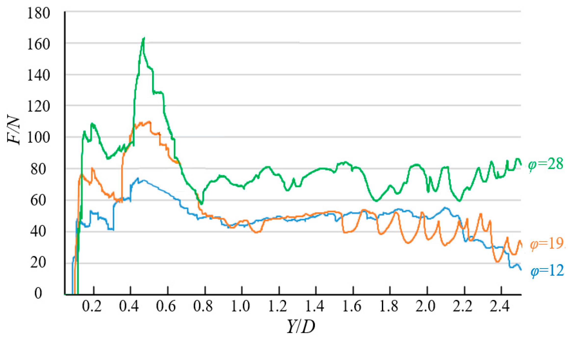
Under shallow burial failure conditions (illustrated in Figure 4), the relationship between pipeline lateral displacement (Y) and resultant load (F) exhibits characteristics that reflect the progressive evolution of soil failure. As the pipeline’s lateral displacement increases from its initial position, the load acting on the pipeline initially demonstrates a nonlinear increase with a steep gradient, reflecting the elastic response of the surrounding soil. Subsequently, the load–displacement relationship exhibits notable post-peak softening behavior. This characteristic load reduction occurs specifically due to progressive shallow burial failure development in the surrounding soil, where shear band formation and propagation toward the surface effectively reduces the soil’s resistance capacity. As displacement continues, the load eventually stabilizes, exhibiting minor fluctuations around a relatively constant residual value that represents the post-failure resistance capacity of the soil.

The parametric results reveal two fundamental relationships: For configurations with identical depth-to-diameter ratio ($H/D$), soil density significantly influences resistance magnitude. Denser sand formations generate greater ultimate and residual loads on pipelines, showing approximately linear proportionality within the tested range. Under constant soil density conditions, peak resistance positively correlates with burial depth ratio, increasing substantially as $H/D$ rises from 1 to 5. This reflects enhanced confining pressure and expanded failure surface area in deeper burial configurations, resulting in greater soil mobilization during lateral displacement.

Load–displacement relationships for pipe–soil lateral interaction under shallow burial conditions with varying soil densities and depth-to-diameter ratios: (a) soil density = 16 kN/m³; (b) soil density = 17.5 kN/m³; (c) soil density = 19 kN/m³.

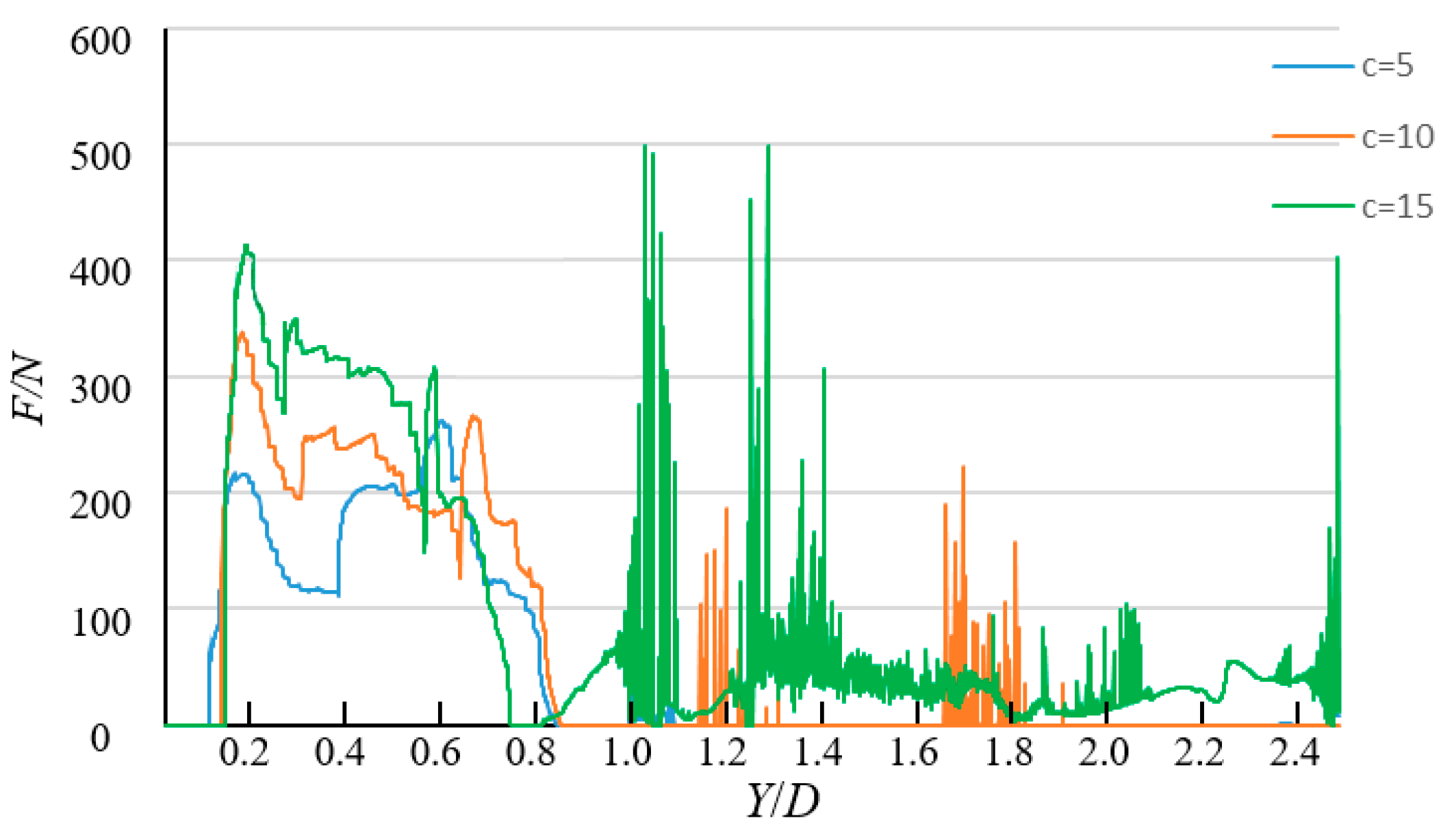
Under deep burial conditions (documented in Figure 5), the variation pattern of soil loads acting on the pipeline maintains similarity with shallow burial behavior in terms of general progression: the relationship between applied load (F) and lateral displacement (Y) follows a pattern characterized by initial load increase, achievement of a distinct peak resistance value, followed by post-peak decline, forming a characteristic mountain-like profile in the load–displacement space. However, detailed analysis between shallow and deep burial response characteristics reveals several differences: (1) The load under deep burial failure modes reaches its peak value at noticeably smaller lateral displacement values compared to shallow burial conditions, indicating more rapid mobilization of ultimate soil resistance under confining conditions characteristic of deep burial configurations. (2) Following achievement of peak resistance, the load stabilizes considerably more rapidly under deep burial conditions, demonstrating reduced post-peak displacement requirements to achieve residual resistance conditions. (3) The stabilized load value under deep burial conditions is quantitatively lower than corresponding values under shallow burial. This observation demonstrates direct correlation with the soil failure patterns, where the failure zone induced by pipeline movement under deep burial configurations approximates a circular shape rather than extending to the surface.

In order to establish the quantitative validation of the model, this investigation conducts detailed comparative analysis between simulation results and experimental measurements. Specifically, the load–displacement relationships under shallow burial conditions for the representative soil density of 16 kN/m³ (illustrated in Figure 4a) are compared with corresponding experimental results obtained by Hao et al. under equivalent geotechnical and geometric conditions. The characteristic progression of load–displacement response observed in experimental measurements is reproduced by the SPH model, capturing the initial nonlinear load increase with displacement, distinct peak resistance achievement, post-peak resistance reduction, and subsequent stabilization around a constant residual value. This pattern reproduction validates the model’s capability to represent the complete load–displacement relationship. Both experimental and computational results demonstrate that peak load magnitude increases with increasing burial depth, with quantitative differences between experimental and numerical results generally remaining below 12% across the tested range, which lies within acceptable engineering tolerance considering inherent variability in geotechnical parameters. The model predicts the stabilized residual resistance values observed experimentally, with deviation generally below 10% across measured configurations.

The validation confirms that the developed SPH model exhibits relatively high accuracy in predicting both qualitative behavioral patterns and quantitative resistance values across diverse burial configurations. Furthermore, the model demonstrates numerical stability characteristics, producing smooth load–displacement curves without artificial oscillations or convergence issues that frequently challenge conventional mesh-based approaches under large deformation conditions.

4. Analysis of Influencing Factors

4.1. Influence of Soil Parameters

To analyze the influence of critical soil parameters on buried pipeline–soil interaction, the investigation maintains consistent reference conditions based on the initial parameters in Table 1, while modifying elastic parameters to better represent typical soil conditions. The bulk modulus (K) and shear modulus (G) are calibrated to 13.33 MPa and 8 MPa, respectively, based on representative values for medium-dense sandy soils in geotechnical literature. A configuration with depth-to-diameter ratio ($H/D$) of 5 and soil density of 17.5 kN/m³ is selected as the baseline scenario for parametric analysis. This configuration represents a transitional burial depth between shallow and deep failure, offering enhanced sensitivity to parameter variations while maintaining relevance to typical pipeline installation conditions. The analysis focuses on two fundamental soil strength parameters—cohesion and internal friction angle—and their effects on pipeline–soil interaction characteristics under controlled conditions.

4.1.1. Internal Friction Angle

When investigating the influence of internal friction angle on the interaction between buried pipelines and surrounding soil, soil cohesion was maintained at zero throughout the analytical process. Comprehensive numerical simulations were conducted with three strategically selected internal friction angle values—12°, 19.8°, and 28°—representing loose, medium-dense, and dense sand conditions, respectively. The simulation results are represented through contour maps of soil deformation patterns illustrated in Figure 6. Surface deformation characteristics show that as the internal friction angle progressively increases from 12° to 28°, the concave depression region developing in the soil above the pipeline becomes increasingly pronounced. Heave formation dynamics indicate the curvature and amplitude of the convex heave feature forming on the soil surface ahead of the pipeline movement direction increases substantially with higher friction angles.

The quantitative load–displacement relationships corresponding to internal friction angles of 12°, 19.8°, and 28°, are presented in Figure 7. These curves provide the soil–pipeline response under varying frictional conditions. These results demonstrate a pronounced correlation between internal friction angle and resistance characteristics: as the internal friction angle progressively increases across the investigated range, both the instantaneous lateral interaction load between the pipeline and soil and the ultimate resistance value increase substantially.

4.1.2. Cohesion

To investigate the influence of soil cohesion on buried pipeline–soil interaction, the internal friction angle is maintained at a constant value of 19.8° throughout the analysis, while cohesion values of 5 kPa, 10 kPa, and 15 kPa are evaluated through sequential simulations. These selected cohesion values span the representative range typically encountered in clay soils from soft to stiff consistency. The simulation results are presented in Figure 8, which illustrates the progressive evolution of failure with increasing cohesion values.

Cohesion fundamentally alters material behavior by establishing tensile strength between soil particles. During pipeline lateral movement, soil in cohesive media maintains structural integrity across gaps behind the pipeline rather than collapsing, resulting in defined failure surfaces with distinct tensile features—a distinction from granular soil response. Soil arching remains evident across all tested cohesion values, though its morphology evolves with increasing cohesion from distributed settlement patterns toward more localized, steeper-sided depression zones, reflecting enhanced capacity to maintain steeper unsupported faces. As cohesion increases from 5 kPa to 15 kPa, void spaces behind the advancing pipeline enlarge, upward crack propagation from the pipeline crown becomes more pronounced, tensile crack definition intensifies, and soil arching features become more pronounced yet localized, reflecting the enhanced structural capacity of highly cohesive materials.

The quantitative load–displacement relationships characterizing pipeline–soil interaction under varying cohesion conditions are presented in Figure 9. These curves provide fundamental response across the investigated cohesions. The fundamental progression pattern demonstrates that as pipeline lateral displacement incrementally increases, the pipe–soil interaction force initially rises, eventually reaching a distinctive peak value representing the ultimate resistance capacity of the cohesive soil. Following peak achievement, the resistance force subsequently declines as progressive failure develops within the soil. However, a critical distinction emerges between cohesive and cohesionless soil response characteristics in the post-peak region: unlike the relatively smooth stabilization observed in sandy soils, where resistance typically converges toward a consistent residual value, the post-peak response in cohesive soils exhibits significant amplitude fluctuations without establishing a stable residual plateau.

This distinctive oscillatory behavior in the post-peak region of cohesive soils likely stems from complex interaction between the cohesive soil and the pipeline. Specifically, the periodic resistance fluctuations appear to correlate with sequential formation and failure of cohesive soil blocks as the pipeline advances, where tensile strength allows temporary development of semi-stable soil structures that subsequently undergo sudden failure when critical stress thresholds are exceeded. This cyclic formation–failure process generates the characteristic sawtooth pattern observed in the load–displacement curves for cohesive materials.

4.2. Vertical Pipe–Soil Interaction Analysis

To analyze the vertical interaction between buried pipelines and surrounding soil media—a loading scenario fundamentally different from lateral movement but equally critical for complete pipeline design—the investigation maintains consistent reference parameters from Table 1 while implementing specific calibrations to elastic moduli (bulk modulus adjusted to 13.33 MPa and shear modulus to 8 MPa) to ensure appropriate representation of soil stiffness characteristics under vertical loading conditions. The parametric investigation incorporates three selected depth-to-diameter ratios ($H/D$ = 3, 8, and 10) spanning both shallow and deep burial configurations, combined with three representative soil densities (16 kN/m³, 17.5 kN/m³, and 19 kN/m³) encompassing loose to dense soil conditions.

The soil deformation and stress distribution patterns during downward pipeline movement are presented in Figure 10. As the pipeline moves progressively downward under prescribed displacement conditions, soil pressure gradually intensifies on both the lower face (directly beneath the pipeline) and lateral sides of the pipeline structure. This pressure distribution reflects progressive soil compression and stress concentration in regions experiencing direct loading from the advancing pipeline. A notable observation distinguishing vertical from lateral interaction is the absence of distinct, well-defined failure surfaces within the soil continuum during vertical pipeline movement. Unlike lateral loading scenarios, where shear bands develop with clear geometric patterns dependent on burial depth, vertical loading generates a more distributed compression zone beneath the pipeline without the formation of discrete failure planes.

The quantitative load–displacement relationships for vertical pipe–soil interactions across diverse conditions are presented in Figure 11. As pipeline vertical displacement (Y) increases, the resultant load follows a characteristic pattern: initial nonlinear increase, peak resistance achievement, and post-peak decline. Soil density significantly influences resistance magnitude, with denser sand generating greater ultimate resistance. Burial depth substantially affects resistance characteristics, with deeper configurations producing higher resistance following a nonlinear trend where gains diminish at higher burial ratios. Notably, larger depth-to-diameter ratios ($H/D$) require smaller vertical displacements to achieve ultimate resistance, reflecting better stress transfer in well-confined conditions. These relationships provide valuable guidance for predicting vertical resistance characteristics in pipeline design applications.

5. Conclusions

This research establishes a computational framework using Smoothed Particle Hydrodynamics (SPH) to analyze pipe–soil interaction, effectively capturing soil failure mechanisms during pipeline movement without mesh distortion limitations. The model successfully reproduces both shallow burial failure (characterized by “V”-shaped shear bands extending to the surface) and deep burial failure (exhibiting localized circular failure zones), with the burial depth-to-diameter ratio ($H/D$) governing failure mode transition—$H/D$ < 5 produces shallow failure, $H/D$ > 10 generates deep burial behavior, and 5 < $H/D$ < 10 shows transitional characteristics. Soil parameters significantly influence resistance: increasing internal friction angle (from 12° to 28°) enhances dilatancy and interlocking effects, while increasing cohesion (from 5 to 15 kPa) introduces complex post-peak behavior with distinctive load fluctuations. The research shows that vertical and lateral pipeline movements mobilize different soil responses, with lateral movement generating defined shear bands, while vertical movement produces distributed compression zones without discrete failure planes; for both directions, increased soil density and burial depth enhance ultimate resistance values. The SPH model demonstrates superior capability in handling large deformations, discontinuous failure surfaces, and complex loading conditions without numerical instabilities, making it valuable for analyzing pipeline response to geohazards such as landslides, fault movements, and ground subsidence, ultimately establishing SPH as an effective tool for predicting soil–pipeline system behavior under diverse geotechnical conditions and loading scenarios in pipeline engineering practice.