Article

Assessment of Reasons for Low Productivity in Ultra-Deep Fractured Tight Sandstone Reservoirs Using Data-Driven Analysis

1
Petrochina Tarim Oilfield Company, Korla 841000, China
2
R&D Center for Ultra-Deep Complex Reservoir Exploration and Development, China National Petroleum Corporation (CNPC), Korla 841000, China
3
Engineering Research Center for Ultra-Deep Complex Reservoir Exploration and Development, Korla 841000, China
4
State Key Laboratory of Oil and Gas Reservoir Geology and Exploitation, Southwest Petroleum University, Chengdu 610500, China
*
Author to whom correspondence should be addressed.
Processes 2025, 13(6), 1793; https://doi.org/10.3390/pr13061793
Submission received: 7 April 2025 / Revised: 23 May 2025 / Accepted: 30 May 2025 / Published: 5 June 2025
(This article belongs to the Section Energy Systems)

Abstract

With the increase in exploration and development, the productivity of some wells in the BD area of Kuqa Depression, Tarim Basin, has failed to meet the expected standards. The underlying causes remain unclear, limiting the optimization of stimulation techniques and hindering production enhancement. Data-driven analysis is a promising approach for post-fracturing evaluation. In this study, a comprehensive database of wells in the BD area was established. The formation and fracturing parameters of post-stimulated wells, Pearson correlation coefficient, multiple linear regression, and machine learning were used to identify the key factors controlling productivity including the pressure coefficient, formation porosity, natural fracture density, and strength of injected fluid. This approach helps reduce the complexity of assessing the causes of low productivity. By parameter comparison and “G” function analysis, the preliminary reasons for low productivity in the BD area were identified as follows: (1) difficulty in forming complex fracture networks due to a low natural fracture density; (2) limited stimulation scope due to a high fracture propagation pressure; (3) a low formation pressure coefficient; and (4) a low well productivity index of peripheral wells. Considering the high calcium content in natural fractures, a composite stimulation method—“pre-acid fracturing + hydraulic fracturing”—is proposed to enhance fracture network connectivity through acid dissolution. By comparing the stimulation performance, it is suggested that hydraulic fracturing should be the main method for reservoirs with a low natural fracture density. For the reservoir with a high natural fracture density, the composite stimulation mode is beneficial to activate calcium-filled natural fractures by acid and reduce the difficulty of injecting proppant to support the fracture network. This study provides a theoretical basis for optimizing fracturing strategies in the BD area.

1. Introduction

Bashijiqike Formation and Baxigai Formation in the BD area of Kuqa Depression are the main gas-producing sandstone reservoirs in Tarim Oilfield, China, which are characterized by a large reservoir depth (4500–8200 m), a high pressure (100–140 MPa), a high temperature (120–140 °C), and the poor physical properties of matrices (the average porosity is 7.3%, and the average permeability is 0.885 mD) [1]. The developed natural fractures are mostly filled with calcium, providing an effective space for the accumulation and seepage of oil and gas. As shown in Table 1, based on the early experience, reservoirs can be roughly classified into three categories (i.e., L = Ⅰ, II, or III) based on the effectiveness assessment of natural fractures. The standard gas productivity per well (Q) (i.e., open flow rate) for each category is set as 2 × 10⁶ m3/d for category I, 1.5 × 10⁶ m3/d for category II, and 1 × 10⁶ m3/d for category III [2]. According to reservoir characteristics, a corresponding recommended stimulation technology is developed. However, with the gradual development of the gas reservoir, conventional stimulation technologies have limitations and challenges in terms of production improvement. Thus, a composite stimulation strategy combining pre-acid fracturing and hydraulic fracturing is proposed, aiming to open up calcium-filled natural fractures through acid dissolution. The mechanisms behind the low productivity per well and the effectiveness of composite stimulation have not been fully understood, resulting in uneven productivity enhancement across wells and a lack of clear guidance for further fracturing parameter optimization.
Data-driven approaches have been widely applied to fracturing analysis. Mahmoud et al. (2020) [3] developed a conductivity prediction model with a machine learning algorithm, and investigated the effects of different mineral compositions and etching patterns on the acid-etched fractures’ conductivity. Zhu et al. (2024) [4] established an AutoGluon-based framework to enable the precise prediction of fracturing parameters, leading to optimized stimulation designs for horizontal wells. The framework has been effectively applied in field operations, such as those in the Xinjiang Oilfield, yielding notable enhancements and operational success. Zhao et al. (2024) [5] investigated the application of data-driven methods for dynamically predicting fracture propagation in horizontal well hydraulic fracturing. By utilizing a ConvLSTM network as the prediction model, they were able to accurately forecast the morphology and location of fracture extensions. Hou et al. (2022) [6] utilized multiple linear regression (MLR), support vector regression (SVR), and artificial neural networks (ANNs) to predict the brittleness index of rocks, thereby significantly reducing the prediction errors in comparison to field measurements, which has been effectively applied in the well and layer selection processes for hydraulic fracturing operations. Amro et al. (2023) [7] employed machine learning methods, including fully connected neural networks (FCNNs), gradient boosting (GB), adaptive boosting (AdaBoost), extreme gradient boosting (XGB), random forest (RF), and decision trees (DTs), to predict the fracturing fluid viscosity. They utilized the particle swarm optimization (PSO) algorithm to optimize the fracturing fluid viscosity under high-salinity formation water conditions. Morozov et al. (2020) [8] leveraged a decision tree model for production forecasting and assessing optimized hydraulic fracturing operation parameters, demonstrating its successful application in the Marcellus Shale Reservoir. The current research on data-driven approaches is predominantly confined to either acid fracturing or hydraulic fracturing individually [9,10], and it has not yet been extended to composite stimulation.
Therefore, based on the formation and fracturing parameters of the post-stimulated wells, this study uses the Pearson correlation coefficient method, multiple linear regression method, and machine learning method to determine the key factors controlling productivity after fracturing. Then, parameter comparison and “G” function analysis are adopted to decipher the reason for low productivity in the BD area. After identifying the causes of low productivity, a composite stimulation technique was proposed based on the fact that the fractured sandstone reservoirs in the BD area are filled with calcium, aiming to explore new technologies for productivity enhancement.

2. Analysis of Main Factors Controlling Productivity

The productivity of gas well after fracturing is simultaneously controlled by formation and fracturing parameters [11]. Taking into account the representativeness, universality, and acquisition difficulty of the selected parameters, porosity (φ), gas saturation (Sg), effective thickness of reservoir (h), pressure coefficient (α), natural fracture density (ρn), angle between natural fracture and maximum horizontal principal stress (θ), density of leak-off drilling fluid (ρm), leak-off volume of drilling fluid (Vl), and maximum hydrocarbon (Cn) are selected as the formation parameters; furthermore, the strength of injected fluid (ql), strength of proppant (qs), general injected flow rate (Qr), and pressure drop rate when the pump stops (Pd) are selected as the fracturing parameters. A total of 52 wells in the BD area are selected considering the parameter integrity, and the statistical parameters of some wells are provided in Table 2. These wells come from different sub-areas, covering the main reservoir levels and productivity and physical property ranges. Due to the large effective thickness span (some >250 m) of target formation in some wells, parameters such as porosity (φ) and gas saturation (Sg) greatly fluctuate, so the thickness-weighted average is chosen as the representative value. For some wells, due to poor wellbore conditions, porosity and other parameters cannot be directly obtained by well logging, so the adjacent well data are selected as their representative values.
Multiple linear regression is a key method for assessing the relative influence of various factors. However, it is crucial to first evaluate the presence of multicollinearity among these factors, as it can lead to unstable coefficient estimates and obscure the independent contribution of each variable. The Pearson correlation coefficient is a statistical measure used to quantify the degree of linear association between two variables. The Pearson correlation coefficient rxy between variables X and Y can be calculated using Equation (1) [12]:
r X Y = n X i Y i X i Y i n X i 2 ( X i ) 2 n Y i 2 ( Y i ) 2
Variables X and Y are positively correlated when 0 < rxy ≤ 1 and negatively correlated when −1 ≤ rxy < 0. In most situation, the linear relationship between the two variables is significant when |rxy| ≥ 0.75, and less obvious when 0.5≤ |rxy| < 0.8. The linear relationship between two variables is weak when 0.3 ≤ |rxy| < 0.5, and can be ignored when |rxy| < 0.3. Based on the established database in the BD area, the Pearson correlation coefficient calculated results are shown in Figure 1. The Pearson correlation coefficients are mostly less than 0.3 and all less than 0.5, indicating that the degree of multicollinearity between different parameters is weak and can be ignored. In addition, the values of the Pearson correlation coefficient between single formation or fracturing parameters and productivity are all less than 0.5, indicating that the correlation between productivity and a single parameter is weak. However, this does not necessarily mean that these parameters have no effect on productivity, because productivity could be controlled by multiple formation and fracturing factors simultaneously. In this case, multiple linear regression is an effective means to comprehensively analyze the weight under the synergistic effect of many factors [13].
Parameters need to be standardized (calculated by Equation (2)) before calculation to eliminate the influence of parameter dimensions when applying multiple linear regression. The conventional multiple linear regression optimizes the loss function (i.e., Equation (3)) by the least square method to find the best regression coefficient and minimize the difference between the predicted and actual data [14]. The results of the conventional multiple linear regression are shown in Equation (4) and Figure 2, and the determination coefficient (R2) of the model reaches 0.51. From the absolute values of each weight coefficient, it can be concluded that general injected flow rate (Qr), pressure coefficient (α), average porosity (φ), natural fracture density (ρn), and the density of leak-off drilling fluid (ρm) have high impact on productivity per well (Q).
X = X μ X σ X
L OLS = i = 1 n ( Q i X i β ) 2
Q = 346.873 + 34.446 × Q r 5.753 × q s 0.675 × q l + 0.102 × V l 1.230 × S g + 12.307 × φ + 167.549 × α + 0.041 × h + 0.943 × θ + 24.658 × ρ m 0.031 × C n 21.994 × ρ n + 0.201 P d
where X′ is the standardized parameter of X; μx is the mean value of X; σx is the standard deviation of X; n is the number of the well; β is the regression coefficient vector, representing the weight of each parameter.
As shown in Equations (5) and (6), the Ridge and Lasso regression model improves the least square method by adding a regularization term related to the coefficient into the loss function [15,16] (Li et al., 2024; Nadeem et al., 2024). The purpose is to reduce the influence of multicollinearity by controlling the regression coefficient, and also to avoid overfitting and improve the stability of the model [17,18]. The results of Ridge regression are shown in Equation (7) and Figure 3, and those of Lasso regression are shown in Equation (8) and Figure 3, with R2 reaching 0.52 and 0.54, respectively. The three multiple linear regression models assessed the same main controlling factors of productivity, but the values of the fitting R2 of the three multiple linear regression models are relatively small, and their accuracy is not positive. Combined with Pearson correlation coefficient, the results showed that the linear correlation between a single formation or fracturing parameter and productivity is poor, so it can be naturally inferred that the productivity of post-fracturing well in the BD area could be a multivariate nonlinear function of statistical parameters.
L R idge = i = 1 n ( Q i X i β ) 2 + λ j = 1 p β j
L Lasso = i = 1 n ( Q i X i β ) 2 + λ j = 1 p | β j |
Q = 230.866 + 27.334 × Q r 7.681 × q s 0.165 × q l + 0.077 × V l 1.167 × S g + 12.876 × φ + 109.346 × α + 0.054 × h + 0.563 × θ + 22.815 × ρ m + 0.017 × C n 16.453 × ρ n + 0.251 P d
Q = 310.76 + 33.305 × Q r 6.639 × q s 0.395 × q l + 0.098 × V l 1.276 × S g + 12.879 × φ + 146.891 × α + 0.049 × h + 0.856 × θ + 24.691 × ρ m 0.046 × C n 21.674 × ρ n + 0.574 P d
where p is the number of variable X.
Machine learning can be used to analyze the weight of influencing factors and additionally to capture the nonlinear relationships without the need for linear relationship assumptions [19,20]. To ensure the reliability of the results, four machine learning models, including random forest, Adaboost, LightGBM, and neural network, are compared. When compared with complex models such as LightGBM and neural networks, random forests and AdaBoost are relatively simpler in structure, tend to perform more stably on small sample datasets, and exhibit lower sensitivity to hyperparameter settings. In contrast, LightGBM and neural networks generally require larger datasets and careful parameter tuning to achieve optimal performance.
Based on the R2 results, K-fold cross-validation (k = 5) is selected to verify the stability and accuracy of the model [21]. The average R2 of random forest, Adaboost, LightGBM, and neural network models with K-fold cross-validation is 0.70, 0.64, 0.76, and 0.78, respectively. Meanwhile, the standard deviation of R2 of random forest, Adaboost, LightGBM, and neural network models is 0.11, 0.09, 0.23, and 0.26, respectively. The average weights of parameters from four machine learning models are shown in Figure 4. Although the factors affecting productivity assessed by different models are disparate, the important factors (i.e., the mean weight of four models > 0.10) that are assessed at the same time include the pressure coefficient (α), average porosity (φ), natural fracture density (ρn), and strength of injected fluid (ql).
Compared with the results of multiple linear regression models, it indicates that the machine learning model can significantly improve the accuracy of prediction. Based on the analysis of the results of the key factors controlling productivity of both machine learning and multiple linear regression, the final key factors controlling productivity in the BD area are pressure coefficient (α), average porosity (φ), and natural fracture density (ρn).

3. Deciphering Reasons for Low Productivity

Based on the established database and the analysis of the results of the key factors controlling productivity, the reasons for low productivity are analyzed by the most direct method, i.e., parameter comparison. As shown in Table 3, the target formations of W1 and W2 both belong to category III, but the difference in productivity between them is nearly 10 times. By comparing the formation parameters of W1 and W2, we can see that the pressure coefficient and average porosity of W1 and W2 are similar, but the natural fracture density of W1 is significantly lower than that of W2. As shown in Figure 5a, statistical results show that there is a positive correlation between productivity and natural fracture density, and natural fracture density is an important factor controlling productivity. In the comparison of the fracturing parameters, the same fracturing technology was adopted for the two wells, with little difference in the strength of injected fluid, strength of proppant, and general injected flow rate. However, the pressure drop rate when the pump of well W1 stops is significantly lower than that of well W2, indicating that the fracture network complexity of well W1 may be smaller. The “G” function is also an important method to assess fracture complexity, and the number of curve tangents represents the natural fracture stages that hydraulic fractures activate [22]. As shown in Figure 5b, based on the fracturing curve of well W1, there is only one tangent line of the curve through the origin determined by the “G” function, indicating that the one-stage natural fracture is activated. Taking the above analysis into consideration, the reason for the low productivity of well W1 is the difficulty to form a complex fracture network due to poorly developed natural fractures.
It can be seen from Table 4 that the target formations of W3 and W4 both belong to category III, but the productivity of W3 is not up to the set standard. When compared with the formation parameters, there is no obvious difference between other parameters except that the natural fracture density of well W3 is relatively larger. When compared with the fracturing parameters, the two wells are both fractured by the same technology, and have the same strength of injected fluid (ql), strength of proppant (qs), and general injected flow rate (Qr). However, the pressure drop rate when the pump (Pd) of W3 stops is slightly lower than that of well W4, indicating that well W3 forms a less complicated fracture network. In addition, it can be seen from Figure 6a that the “G” function of W3 after fracturing has no tangential line, indicating that natural fractures have not been activated. This may be because the angle between natural fracture and the maximum horizontal principal stress (θ) of W3 is larger, so natural fractures are more difficult to activate. Based on the fracturing curve of W3, it can be seen in Figure 6b that the fracture propagation pressure gradient of W3 assessed by a lift flow rate is as high as 2.31 MPa/100 m, and it can be seen from Figure 6c that the fracture propagation pressure gradient is negatively correlated with the productivity, which further proves that the reason for the low productivity of well W3 is the large angle between natural fracture and the maximum horizontal principal stress and the fracture propagation pressure gradient, which makes it difficult to activate natural fractures.
Table 5 indicates that the target formations of W5 and W6 both belong to category III, but the productivity of W6 is not up to the set standard. When compared with the formation parameters of the adjacent well W5, W6 has a higher logging porosity and a higher natural fracture density, indicating the better physical properties of the near-well position. When compared with the fracturing parameters of W5 and W6, well W5 has lower strength of injected fluid (ql), strength of proppant (qs), and general injected flow rate (Qr). The productivity of W5 after fracturing should be smaller, but the pressure drop rate when the pump stops (Pd) for well W5 is almost twice that of W6, indicating that the fracture network formed in W5 might be more complex. As shown in Figure 7a, based on the fracturing curve of W6, there is a tangent line in the “G” function, indicating that W6 activates only one-stage natural fractures. As shown in Figure 7b, according to the statistics of the shut-in pressure after blowout among adjacent wells after fracturing, W6 has the lowest shut-in pressure value (70.96 MPa), and the pressure recovery time of W6 is also relatively long (Figure 7c), which indicates that the far-well supply capacity of the target layer of W6 is poor. Based on the above analysis, it is concluded that the low productivity of W6 is caused by the poor physical properties of a position far from the wellbore.
As shown in Table 6, the target formations of wells W8 and W7 both belong to category III. W7 meets the set productivity standard, but W8 fails. By comparing the formation parameters of W7 and W8, it is evident that the natural fracture density (ρn) of W7 is smaller, and its leak-off volume of drilling fluid (Vl) is also smaller, so the productivity of W8 might be higher when other parameters are similar, but the formation pressure coefficient of W8 is significantly lower than that of W7. By comparing the fracturing parameters of W7 and W8, the stimulation technology of the two wells adopted are both “pre-acid + temporary plugging fracturing” with almost similar strength of injected fluid (ql), strength of proppant (qs), and general injected flow rate (Qr), but the pressure drop rate of W7 when the pump stops (Pd) is larger. In addition, W8 is located at the edge of the anticline and has poor formation energy, which is consistent with the occurrence of water in the later production period. Therefore, the reasons for the low productivity of W8 are that it is located at the structural edge and the formation energy is relatively low.

4. Potential Technology for Low-Productivity Well

Due to the limitations and challenges of conventional stimulation mode in the late stage of development in the BD area, a composite stimulation mode (i.e., a pre-acid fracturing is implemented before the hydraulic fracturing) is proposed in combination with the characteristics of developed calcium-filled natural fractures. The purpose of this novel stimulation technology is to make use of the characteristic that acid can quickly dissolve calcium in order to enhance the communication between natural fractures. From Table 7, W9 and W10 both belong to category III, with little difference in the formation pressure coefficient, average porosity, and natural fracture density, but the productivity of W9 after fracturing is significantly lower than that of well W10. When the fracturing parameters of the two wells are compared, they both adopt multi-stage fracturing, and W10 adopts hydraulic fracturing, while well W9 adopts composite stimulation. In addition, the strength of injected fluid (ql), strength of proppant (qs), and general injected flow rate (Qr) of the two wells show inconspicuous difference. However, the productivity of W9 is nearly 1.7 times that of W10, and the pressure drop rate is 3 times that of W10, which reflects the strong ability of composite stimulation to activate calcium-filled natural fractures.
According to the application results of composite stimulation in category I, II, and III reservoirs (Figure 8), the production increase due to composite stimulation in category I and II reservoirs is significantly greater than that in category III reservoirs, indicating that the development degree of natural fractures is still the key factor affecting the performance of composite stimulation. In addition, it can be seen from Figure 9 that the productivity adopting composite stimulation is positively correlated with the strength of injected fluid (ql), strength of proppant (qs), and general injected flow rate (Qr). Therefore, the production increase due to composite stimulation is jointly controlled by the formation and fracturing parameters. To further study the reservoir adaptability of the novel technology, the performance of composite stimulation under different natural fracture densities is simulated based on the basic data of well W9.
According to Figure 10a, in reservoirs with a low natural fracture density, the injected volume of acid has limited influence on the conductivity, stimulation volume, and fracture length. When the volume of acid exceeds 40 m3, the increase rate of stimulation volume and fracture length decreases significantly with the increase in acid volume. Small acidizing processes could be implemented to increase the stimulation volume prior to the main hydraulic fracturing. From Figure 10b, in reservoirs with a high natural fracture density, increasing the injected volume of acid is conducive to expanding the stimulation volume and conductivity. Even if the injected volume of acid reaches 800 m3, the increase rate of the stimulation volume and conductivity with the increase in acid volume does not significantly slow down. Therefore, in reservoirs with a high natural fracture density, the volume of acid can be expanded with “pre-acid fracturing + hydraulic fracturing” (i.e., composite stimulation) to maximize the activation of natural fractures and to increase the stimulation volume and the impact range.

5. Conclusions

Based on the established database of the post-fracturing well in the BD area, the key factors controlling productivity are firstly analyzed. Then, four types of reasons for single-well low productivity are mainly proposed based on parameter comparison and “G” function analysis. Eventually, according to the characteristics of the fractured sandstone reservoir, the composite stimulation mode is put forward, and the reservoir adaptability of composite stimulation is studied. The conclusions of this study are as follows:
(1)
The key factors controlling productivity in the BD area include pressure coefficient, porosity, and natural fracture density.
(2)
The reasons for the low productivity of ultra-deep fractured tight sandstone in the BD area include the following: (1) difficulty in forming a complex fracture network due to a low natural fracture density; (2) a limited stimulation scope due to a high fracture propagation pressure; (3) a low formation pressure coefficient; and (4) the poor physical properties at far-well positions.
(3)
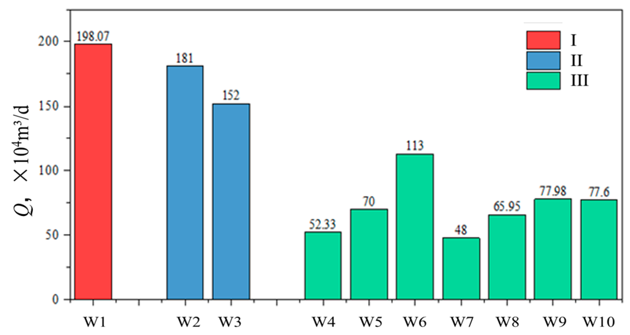
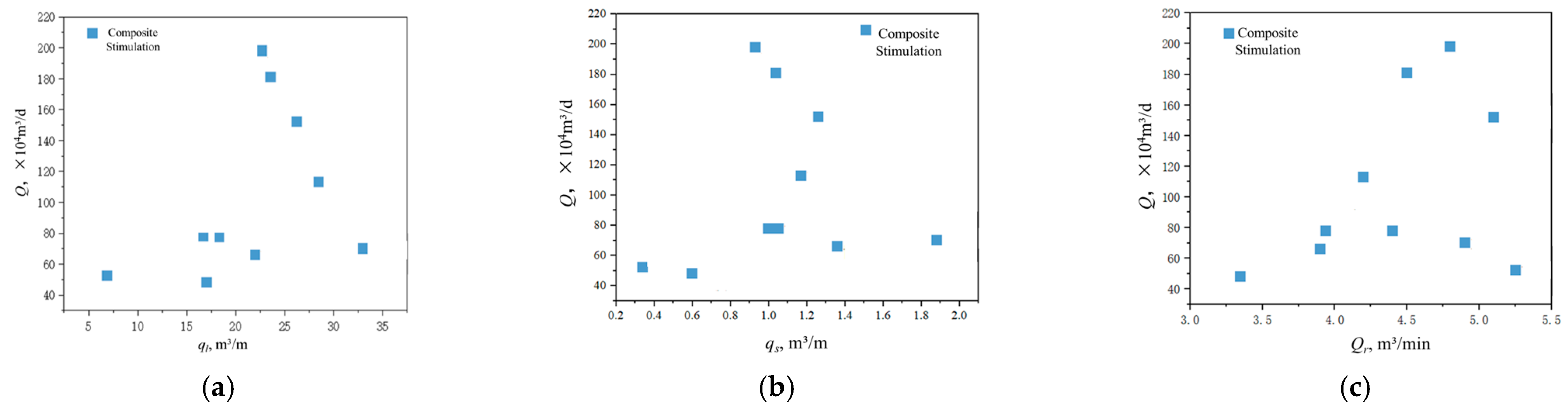
The development degree of natural fractures is still a key factor affecting the performance of composite stimulation.
(4)
For reservoirs with a low natural fracture density, hydraulic fracturing should be the main method used for enhancing the fractures, and small-scale acidification could be implemented for activating the fractures; for reservoirs with a high natural fracture density, composite stimulation shows great potential to increase productivity.

Author Contributions

Conceptualization, F.P.; Formal analysis, Z.L.; Investigation, J.L.; Resources, J.Z. and D.D.; Writing—original draft, Z.L.; Writing—review & editing, B.G.; Supervision, F.P. and J.P. All authors have read and agreed to the published version of the manuscript.

Funding

This research received no external funding.

Data Availability Statement

The original contributions presented in this study are included in the article. Further inquiries can be directed to the corresponding author.

Conflicts of Interest

Authors Fen Peng, Jianping Zhou, Jianxin Peng, Junyan Liu and Dehai Deng were employed by the companies Petrochina Tarim Oilfield Company and CNPC. The remaining authors declare that the research was conducted in the absence of any commercial or financial relationships that could be construed as a potential conflict of interest.

References

  1. Wang, Z.; Wang, C.; Xu, K.; Zhang, H.; Chen, N.; Deng, H.; Hu, X.; Yang, Y.; Feng, X.; Du, Y.; et al. Characteristics and Control Factors of Tectonic Fractures of Ultra-deep Tight Sandstone: Case Study of the Lower Cretaceous reservoir in Bozi-Dabei area, Kuqa Depression, Tarim Basin, China. J. Nat. Gas Geosci. 2023, 8, 439–453. [Google Scholar] [CrossRef]
  2. Wang, C.; Li, H.; Chen, D.; Chen, B.; Liu, L.; Luo, M. Porosity Structure Characteristics and Influencing Factors Analysis of Basijiqike Tight Sandstone Reservoir in Keshen Gasfield. Bull. Geol. Sci. Technol. 2018, 37, 70–77. (In Chinese) [Google Scholar]
  3. Mahmoud, D.; Zeeshan, T.; Murtada, S.; Hamed, A.; Mohamed, M.; Dhafer, A. Data-Driven Acid Fracture Conductivity Correlations Honoring Different Mineralogy and Etching Patterns. ACS Omega 2020, 5, 16919–16931. [Google Scholar]
  4. Zhu, Z.; Hsu, M.; Kun, D. A Data-Driven Workflow for Prediction of Fracturing Parameters with Machine Learning. Therm. Sci. 2024, 28, 1085–1090. [Google Scholar] [CrossRef]
  5. Zhao, M.; Yuan, B.; Liu, Y. Dynamic prediction of fracture propagation in horizontal well hydraulic fracturing: A data-driven approach for geo-energy exploitation. Geoenergy Sci. Eng. 2024, 241, 213182. [Google Scholar] [CrossRef]
  6. Hou, L.; Ren, J.; Fang, Y. Data-driven optimization of brittleness index for hydraulic fracturing. Int. J. Rock Mech. Min. Sci. 2022, 159, 105207. [Google Scholar] [CrossRef]
  7. Amro, O.; Zeeshan, T.; Murtada, S. Enhancing Fracturing Fluid Viscosity in High Salinity Water: A Data-Driven Approach for Prediction and Optimization. Energy Fuels 2023, 37, 13065–13079. [Google Scholar]
  8. Morozov, A.; Popkov, D.; Duplyakov, V. Data-driven model for hydraulic fracturing design optimization: Focus on building digital database and production forecast. J. Pet. Sci. Eng. 2020, 194, 107504. [Google Scholar] [CrossRef]
  9. Zeng, F.; Hu, D.; Zhang, Y. Research on data-driven intelligent optimization of fracturing treatment parameters for shale oil horizontal wells. Pet. Drill. Tech. 2023, 51, 78–87. [Google Scholar]
  10. Yang, J.; Wang, Q.; Zhou, Q. Evaluating staged acid fracturing of horizontal wells in carbonate gas reservoirs based on GBDT algorithm. Nat. Gas Explor. Dev. 2023, 46, 84–91. [Google Scholar]
  11. Sun, F.; Yao, Y.; Li, G.; Qu, S.; Zhang, S.; Shi, Y.; Xu, Z.; Li, X. Effect of Pressure and Temperature of Steam in Parallel Vertical Injection Wells on Productivity of a Horizontal Well During the SAGD Process: A Numerical Case Study. In Proceedings of the SPE International Heavy Oil Conference and Exhibition, Kuwait City, Kuwait, 10–12 December 2018. [Google Scholar]
  12. Carolina, S.; Garfias, D.; Mario, F. Acid dissolution of ultrathin glass-ceramic and its correlation with flexural strength. J. Prosthet. Dent. 2022, 128, 1084–1088. [Google Scholar]
  13. Mardani-Fard, H.A. Principal simple linear regression. Hacet. J. Math. Stat. 2024, 53, 524–536. [Google Scholar] [CrossRef]
  14. Wang, Y.; Huang, Q.; Yao, Z.; Zhang, Y. On a class of linear regression methods. J. Complex. 2024, 82, 101826. [Google Scholar] [CrossRef]
  15. Li, H.; Niu, C. Optimal subsampling for high-dimensional ridge regression. Knowl.-Based Syst. 2024, 286, 111426. [Google Scholar] [CrossRef]
  16. Nadeem, A.; Muteb, F.; Muhammad, S. Mitigating Multicollinearity in Regression: A Study on Improved Ridge Estimators. Mathematics 2024, 12, 3027. [Google Scholar] [CrossRef]
  17. Mei, Z.; Shi, Z. On LASSO for high dimensional predictive regression. J. Econom. 2024, 242, 105809. [Google Scholar] [CrossRef]
  18. Mayur, V.; Joab, R. Numerical properties of solutions of LASSO regression. Appl. Numer. Math. 2024, 208, 297–309. [Google Scholar]
  19. Hu, S.; Sheng, M.; Qin, S. An unsupervised cluster model of formation fracability based on drill-log data and its application to fracture optimization. Pet. Sci. Bull. 2023, 8, 767–774. [Google Scholar]
  20. Sheng, M.; Zhang, J.; Zhang, Y. A new data-driven effectiveness evaluation model of temporary plugging fracturing for horizontal wells. Nat. Gas Ind. 2023, 43, 132–140. [Google Scholar]
  21. Trung, T.; Truong, T.; Tran, V.; Ngo, H.; Dao, Q.; Nguyen, T.; Hoang, K. Virtual Multiphase Flowmetering Using Adaptive Neuro-Fuzzy Inference System (ANFIS): A Case Study of Hai Thach-Moc Tinh Field, Offshore Vietnam. SPE J. 2022, 27, 504–518. [Google Scholar] [CrossRef]
  22. Padmakar, A.S. Geomechanics Coupled Reservoir Flow Simulation for Diagnostic Fracture Injection Test Design and Interpretation in Shale Reservoirs. In Proceedings of the SPE Annual Technical Conference and Exhibition, New Orleans, LA, USA, 29 September–2 October 2013. [Google Scholar]
Figure 1. Pearson correlation coefficient between productivity and statistical parameters.
Processes 13 01793 g001
Figure 2. Multiple linear regression prediction results.
Processes 13 01793 g002
Figure 3. Ridge regression (left) and Lasso regression (right) prediction results.
Processes 13 01793 g003
Figure 4. Comparison of results of machine learning models.
Processes 13 01793 g004
Figure 5. Effect of natural fracture density on productivity: (a) statistical results of natural fracture density and (b) “G” function of well W1.
Processes 13 01793 g005
Figure 6. Analysis of fracturing parameters of W3: (a) “G” function of well W3; (b) step rate assessment of W3; and (c) correlation between propagation pressure gradient and productivity.
Processes 13 01793 g006
Figure 7. Analysis of fracturing parameters of W5: (a) “G” function of well W6; (b) shut-in pressure; and (c) shut-in pressure buildup time of W6 and W5.
Processes 13 01793 g007
Figure 8. Comparative analysis of composite stimulation results in different reservoir types.
Processes 13 01793 g008
Figure 9. Effect of fracturing operation parameters on effectiveness of composite stimulation: (a) strength of injected fluid; (b) strength of proppant; and (c) general injected flow rate.
Processes 13 01793 g009
Figure 10. Effect of pad acid volume on results of composite stimulation: (a) reservoirs with low natural fracture density and (b) reservoirs with high natural fracture density.
Processes 13 01793 g010
Table 1. Basis of reservoir classification of Bashijiqike and Baxigai Formations in BD area.
Reservoir (L)IIIIII
Fracture
characteristics
The longitudinal penetration of reservoirs on a large scale;
semi-filled or unfilled tensile fractures are mainly developed, and the fracture aperture is large.
Fractures are rarely developed and well filled.
Imaging
logging
Fracture density: >0.4 m−1
Standard deviation of θ: >25°
Fracture density: >0.3 m−1
Standard deviation of θ: 20–25°
Fracture density: <0.3 m−1
Standard deviation of θ: <20°
Leak-off
characteristics
Fluid density: 0.1–0.2 g/cm3
Leak-off volume: 100–1200 m3
5–15 points uniformly distributed along the wellbore
Fluid density: 0.15–0.25 g/cm3
Leak-off volume: 100–300 m3
3–5 points uniformly distributed along the wellbore
Fluid density: 0.2–0.3 g/cm3
Leak-off volume: <500 m3
Single-point leak-off or no leak-off
Stimulation
technology
Small-scale acidizingLarge-scale acid fracturing or proppant fracturingProppant fracturing
Stimulation mechanismRemoving damage in the natural fractureActivating the natural fractureForming artificial fractures
Table 2. Statistical parameters of some wells in database.
WellLQαφSghVlρmCnρnθqlqsQrPd
104 m3/d/%%mm3g/cm3%m−1°m3/mm3/mm3/minMPa/min
W1III107.81.796.064.930765.91.852.40.72258.800.383.60.22
W2I201.01.807.968.1285221.11.914.20.79256.780.294.20.33
W3III67.81.796.265.01008.51.9063.50.683014.580.313.30.18
W4II128.01.766.168.7103104.31.925.40.511013.290.684.10.20
W5III12.81.746.366.2460.00.001.80.05257.700.343.30.47
W6III192.61.707.366.411418.01.883.10.413011.540.684.50.29
W7III189.11.717.467.012814.91.885.20.592514.840.884.10.32
W8III232.01.794.169.5919.71.8819.50.793020.351.173.70.48
W9I200.61.497.267.182148.01.7825.10.853019.961.285.00.56
W10I201.41.797.368.3115117.41.907.80.352515.031.113.90.34
W11III69.31.786.664.21190.01.8811.50.521213.150.432.90.78
W12II66.81.247.368.64385.61.722.42.702031.811.704.40.49
W13III52.31.346.067.184298.01.634.50.53506.930.345.20.50
W14III271.91.966.961.9130.01.9710.90.643036.992.144.80.24
W15II165.41.968.171.74018.42.038.40.703036.991.254.70.40
W16I202.91.887.067.892117.22.007.20.50157.680.504.10.50
W17I198.11.566.264.275178.71.5438.80.666822.730.934.80.29
W18II182.51.526.064.08774.21.6110.10.884022.331.125.20.25
W19III81.11.736.561.21320.01.851.90.40436.080.253.50.38
W20III47.91.674.755.0977.21.804.50.14259.660.393.70.39
W21II330.01.716.864.97738.21.847.90.25455.860.334.00.6
W22III126.81.587.264.810310.92.2026.50.162512.550.794.50.54
W23III22.61.565.264.7562.92.205.20.072020.041.224.00.41
W24III66.91.957.564.6170.01.973.31.511545.713.145.40.18
W25II181.91.826.365.52178.91.859.20.652534.412.194.30.33
W26III88.31.587.165.52391.21.685.20.51254.120.153.80.42
Table 3. Comparison of formation and fracturing parameters between W1 and W2.
WellLQαφSghVlρmρnθStimulation TechniqueqlqsQrPd
/104 m3/d/%%mm3g/cm3m−1°/m3/mm3/mm3/minMPa/min
W1III22.61.565.364.7562.92.20.0720Mechanical staged fracturing20.031.224.00.41
W2III235.81.676.664.5631.21.70.3215Mechanical staged fracturing28.081.494.40.82
Table 4. Comparison of formation and fracturing parameters between W3 and W4.
WellLQαφSghVlρmρnθStimulation TechniqueqlqsQrPd
/104 m3/d/%%mm3g/cm3m−1°/m3/mm3/mm3/minMPa/min
W3III67.81.796.4651008.51.90.6845Mechanical staged fracturing11.570.514.30.18
W4III192.61.717.26611418.01.90.4130Mechanical staged fracturing14.530.654.50.30
Table 5. Comparison of formation and fracturing parameters between W5 and W6.
WellLQαφSghVlρmρnθStimulation TechniqueqlqsQrPd
/104 m3/d/%%mm3g/cm3m−1°/m3/mm3/mm3/minMPa/min
W5III103.01.565.564.75601.80.2020Mechanical staged fracturing20.031.224.00.41
W6III77.61.675.164.56301.70.2315Mechanical staged fracturing28.081.494.40.82
Table 6. Comparison of formation and fracturing parameters between W7 and W8.
WellLQαφSghVlρmρnθStimulation TechniqueqlqsQrPd
/104 m3/d/%%mm3g/cm3m−1°/m3/mm3/mm3/minMPa/min
W7III330.01.716.864.97738.21.80.2545Pad acid + diversion fracturing5.850.334.00.60
W8III52.31.346.067.184298.01.60.5350Pad acid + diversion fracturing6.940.345.20.51
Table 7. Comparison of formation and fracturing parameters between W9 and W10.
WellLQαφSghVlρmρnθStimulation TechniqueqlqsQrPd
/104 m3/d/%%mm3g/cm3m−1°/m3/mm3/mm3/minMPa/min
W9III113.01.787.362.3880.01.80.7625Mechanical multi-stage composite stimulation23.500.964.20.59
W10III67.81.796.265.01008.51.90.7030Mechanical multi-stage proppant fracturing21.730.873.90.18
Disclaimer/Publisher’s Note: The statements, opinions and data contained in all publications are solely those of the individual author(s) and contributor(s) and not of MDPI and/or the editor(s). MDPI and/or the editor(s) disclaim responsibility for any injury to people or property resulting from any ideas, methods, instructions or products referred to in the content.

