Abstract
Addressing the critical challenges of sealing integrity and operational optimization in aquifer gas storage (AGS), this study focuses on a block within the Qianjiang Basin to systematically investigate geological modeling and injection–production strategies. Utilizing 3D seismic interpretation, drilling, and logging data, a stochastic geological modeling approach was employed to construct a high-resolution 3D reservoir model, elucidating the distribution of reservoir properties and trap configurations. Numerical simulations optimized the gas storage parameters, yielding an injection rate of 160 MMSCF/day (40 MMSCF/well/day) over 6-month-long hot seasons and a production rate of 175 MMSCF/day during 5-month-long cold seasons. Interval theory was innovatively applied to assess fault stability under parameter uncertainty, determining a maximum safe operating pressure of 23.5 MPa—12.3% lower than conventional deterministic results. The non-probabilistic reliability analysis of caprock integrity showed a maximum 11.1% deviation from Monte Carlo simulations, validating the method’s robustness. These findings establish a quantitative framework for site selection, sealing system evaluation, and operational parameter design in AGS projects, offering critical insights to ensure safe and efficient gas storage operations. This work bridges theoretical modeling with practical engineering applications, providing actionable guidelines for large-scale AGS deployment.
1. Introduction
Natural gas is used in an increasing amount of energy applications due to its complete combustion, low pollution, and large global reserves. However, natural gas usage is characterized by typical seasonal and temporal differences [1,2], meaning that the amount of gas used in the summer is significantly less than that used in the winter and that the amount used at different times on the same day is also significantly different. Underground gas storage can effectively adjust the balance of the supply and demand of natural gas over different periods. Compared with other natural gas storage methods, it has the advantages of a large gas storage capacity, safe and reliable nature, stable gas supply, and economic and reasonable use effects [3]. At the same time, as a strategic energy reserve, a reasonable amount of natural gas reserves also have a far-reaching impact on China’s energy strategy [4,5], so the construction of gas storage has been widely used all over the world as an important part of the development of the oil and gas industry. In 2016, natural gas consumption reached 3.5 trillion cubic meters, accounting for 24% of primary energy consumption, second only to oil (33%) and coal (28%) [6], while the total workload of underground storage reservoirs built so far is 378 billion m3, accounting for only 10.8%, and about 715 underground gas storage facilities have been built worldwide, with a total of 23,007 gas extraction wells and a total working gas volume of 3930 × 108 m3 [7]. Of the three main types of gas storage reservoirs, the depleted reservoir type has the largest ratio of approximately 68%, followed by the aquifer type at 19%, and the salt cavern type at about 12% [8,9]. North America and the CIS have the largest percentages of gas storage, at 35% and 39% respectively, followed by Europe at 25% and other regions at 2% of the world’s total [10]. As of 2018, only 25 underground gas storage facilities have been built and put into operation in China, constructed by two leading state-owned oil companies. The peak shaving gas consumption accounts for only 1.7% of the total annual natural gas consumption, which is 11% higher than the world average. The 8% difference is significant, and there is a huge gap in gas storage capacity, which cannot meet the total peak demand for natural gas in China [11,12]. As of 2021, China’s natural gas consumption has reached 3726 × 108 m3, with a year-on-year increase of 420 × 108 m3, reaching a historical high. Compared with the natural gas production of 2051 × 108 m3 that year, the supply–demand gap has reached 1675 × 108 m3, and all of it relies on imports. External dependence on natural gas has reached 44.9% [13]. Aquifer reservoirs are commonly utilized for underground gas storage. They provide a suitable environment due to their porous and permeable nature, allowing for efficient gas production and injection [14,15]. The natural geological structure of aquifers helps to maintain gas pressure and integrity [16]. This storage method offers benefits, such as increased energy security, flexibility in the gas supply, and reduced price volatility.
2. Methods and Results
The main research content are as follows: (1) Geological Modeling and Geomechanical Analysis; (2) Maximum Operating Pressure Prediction; (3) Fractal Seepage Mechanism Modeling; and (4) Non-Probabilistic Reliability Assessment
2.1. Geomodelling Methods of Aquifer Reservoir
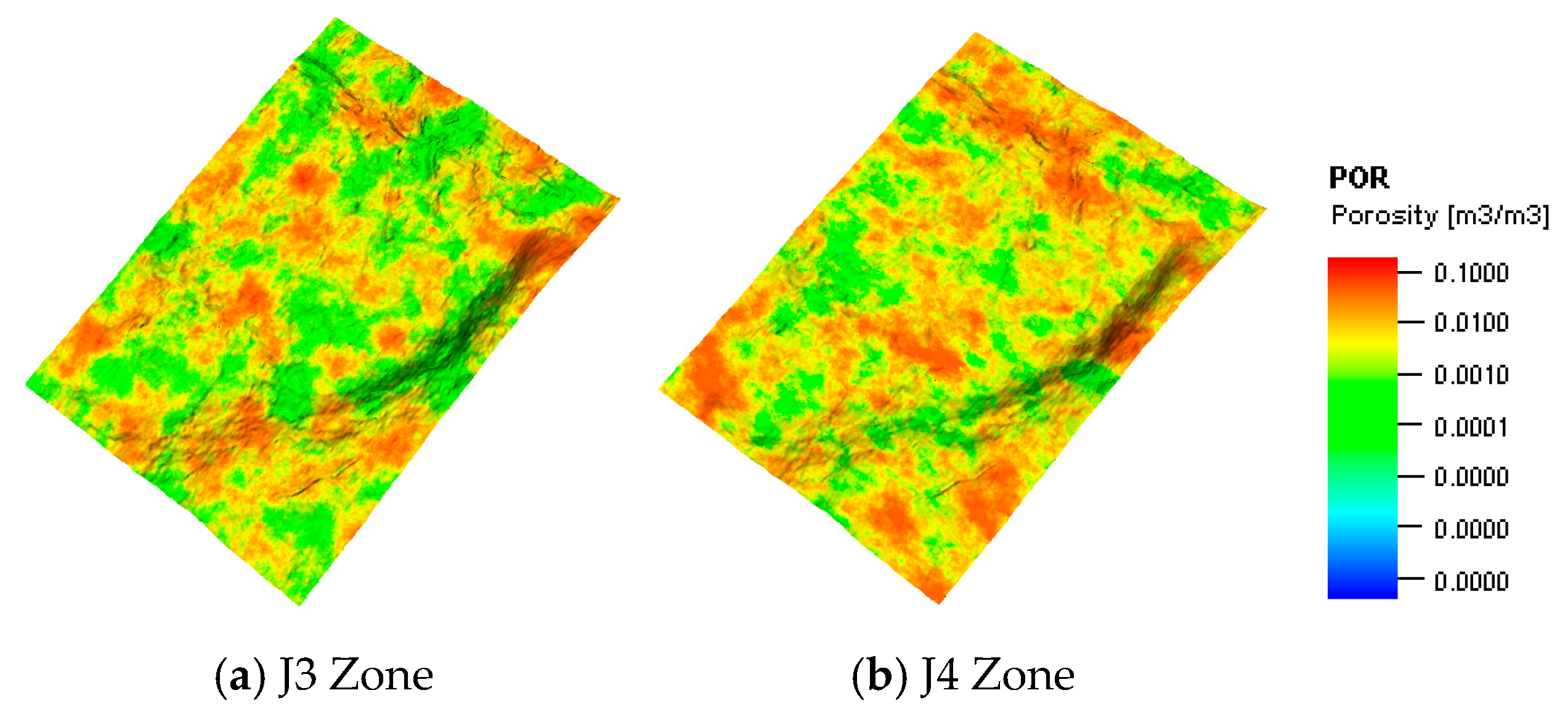
Based on aquifer logging data, sedimentary microfacies, and seismic and other constraint data, we conducted research on pore permeability modeling. Using phase-controlled modeling to analyze the variation function separately, with the well point physical property parameters as conditional data, and taking into account prior geological knowledge, such as sedimentary microfacies and source direction, we conducted an experimental variation function analysis in small layers and phase zones. We constructed a three-dimensional porosity distribution model based on facies-controlled modeling. By integrating logging data (porosity range 0.10~0.15), seismic attributes (wave impedance inversion volume), and a variogram analysis (range 800~1200 m), the model reveals the heterogeneity of reservoir porosity. The high porosity area (>0.13) is mainly distributed in the channel sand body in the sedimentary microfacies, and the low porosity area (<0.11) corresponds to the argillaceous interlayer or tight cemented belt. The lateral constraint of the seismic attributes significantly improves the prediction accuracy between wells, and the model resolution is up to 50 m × 50 m, which meets the requirements for a reservoir dynamic simulation.
In order to elucidate the geological model further, a meticulous examination of the porosity and permeability features is imperative. This necessitates a comprehensive interpretive analysis that correlates the high-resolution logging data with both the porosity models and seismic attributes. By leveraging advanced statistical and geostatistical techniques, such as sequential Gaussian simulations and coordinated Kriging, a sophisticated porosity model was constructed, delivering enhanced accuracy in predictive analytics. Subsequently, the integration of these detailed porosity analyses with the permeability model provided by stochastic geological modeling augments the geological framework, solidifying the interpretations of subsurface fluid flow. Moreover, the incorporation of seismic attribute volume data as a modeling constraint substantiates the geological model’s reliability, thereby granting a robust foundation for appraising the reservoir’s performance. An analysis was conducted for porosity attribute models as shown in Figure 1 and Figure 2.
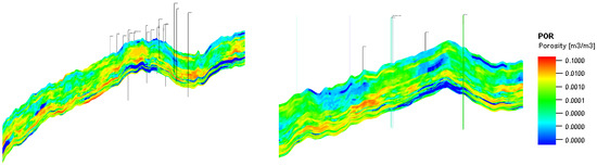
Figure 1.
Profile diagram of aquifer porosity model.

Figure 2.
Layered schematic diagram of aquifer porosity model.
Layered display of porosity model:
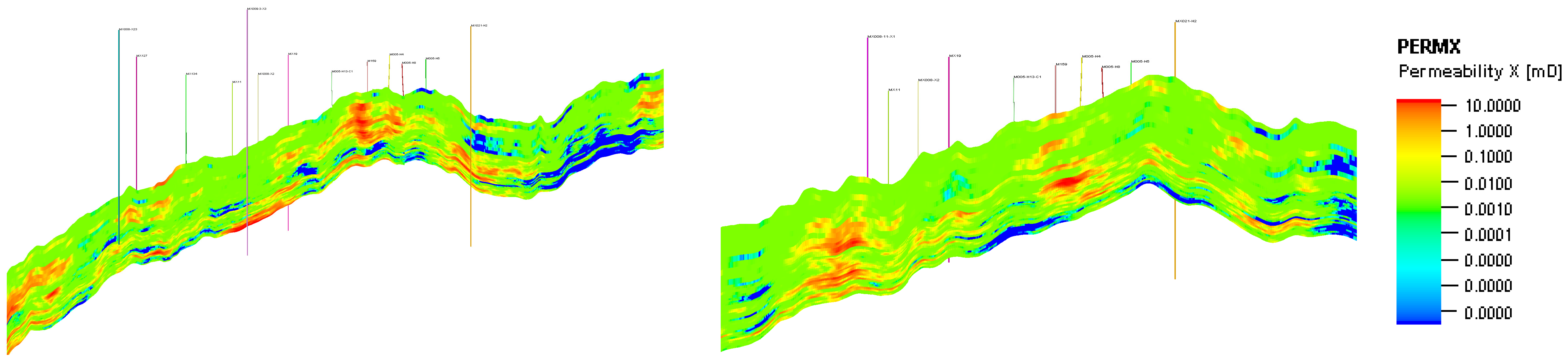
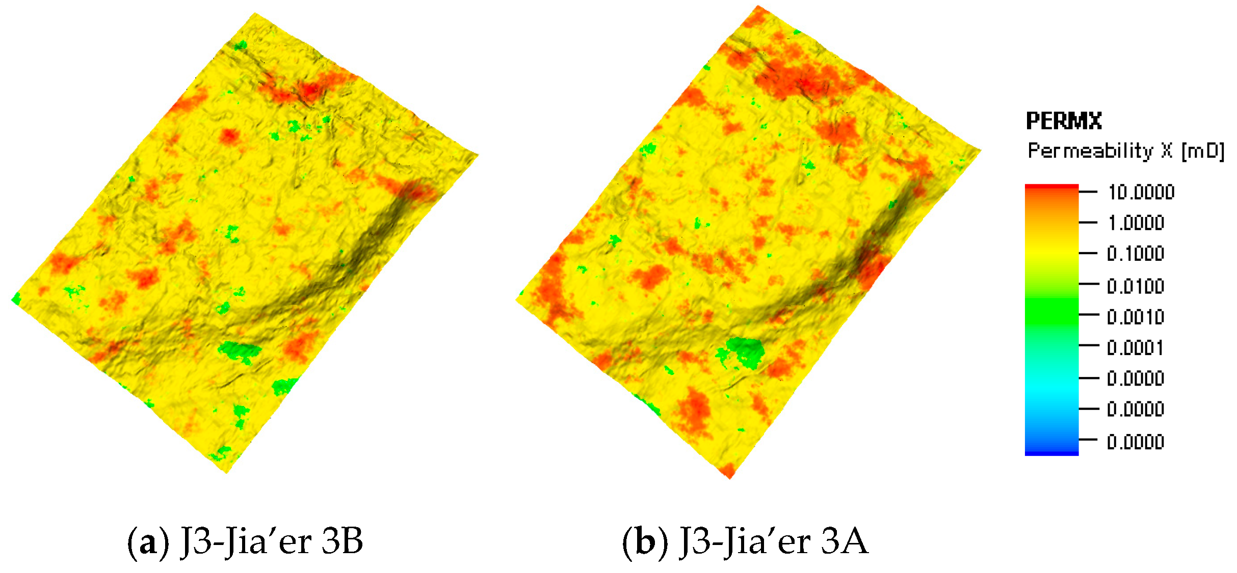
Based on logging data from aquifers, porosity models, and seismic attribute volume data, modeling research was conducted, and a permeability model for the Jia’er reservoir was constructed using a fusion method of coordinated constraint deterministic modeling and random interpolation modeling. We constructed a porosity model using algorithms, such as sequential Gaussian and coordinated Kriging, and applied seismic attribute volumes for modeling constraints. A geological model of aquifer permeability was established using stochastic geological modeling. This involves combining coordinated constraint deterministic modeling and random interpolation modeling, guided by logging data, porosity models, and seismic attribute volume data. Algorithmic techniques like sequential Gaussian and coordinated Kriging facilitate the creation of a comprehensive porosity model. The method is as shown in Figure 3 and Figure 4.

Figure 3.
Profile diagram of aquifer permeability model.
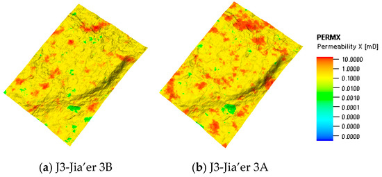
Figure 4.
Layered schematic diagram of aquifer permeability model.
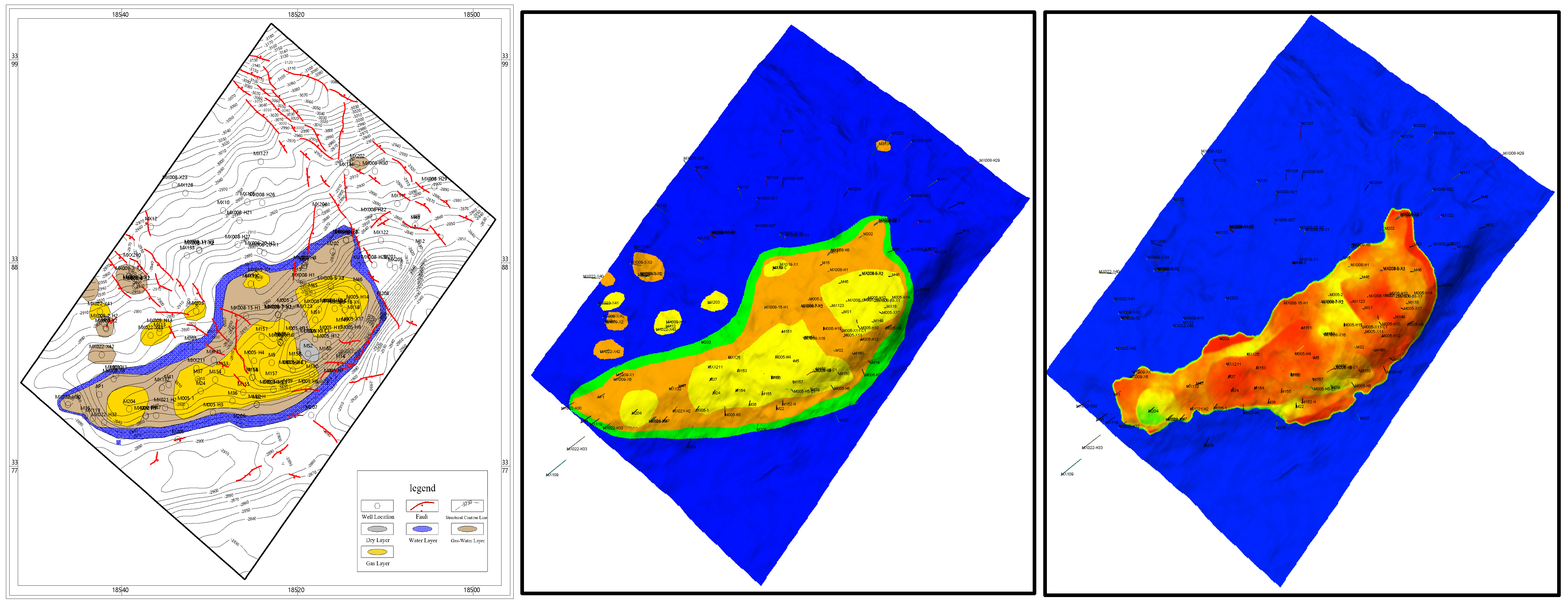
The gas–water interface within the Jia’er reservoir is predicated on an integrative analysis that amalgamates the gas–water transition zone model pattern diagram with empirical logging data. This confluence of data allows for a precise demarcation of the transition zone, which has been quantitatively defined as spanning between 7.3 and 8.1 m. This delineation is critical for understanding the distribution and phase behavior of hydrocarbons in the reservoir, as it reflects the subtle gradations in fluid saturation that inform both the static and dynamic models of the reservoir. This is shown in Figure 5 and Figure 6.

Figure 5.
Schematic diagram of gas–water transition zone in aquifer reservoir.

Figure 6.
Gas–water distribution interface and saturation model of aquifer.
Employing an integration of the gas–water distribution model pattern diagram and corroborative logging data furnishes a substantive framework for delineating the gas–water interface within the reservoir. To ascertain the free-water level height, a meticulously rendered saturation zoning model was employed, which coalesces with the refinement proffered by fine drawing results. This method provides a robust determination of the free-water level height, which is instrumental in comprehending the reservoir’s fluid distribution dynamics and the hydrostatic pressure differentials across the hydrocarbon-bearing layers, as shown in Figure 6.
2.2. Establishment of Numerical Model
2.2.1. Establishment of Grid System
- (1)
- Principles for establishing grid system
Based on the principle of “using as few grids as possible without affecting the accuracy”, the grids in the geological model were discretized. Several aspects should be considered, including geometric characteristics. To achieve the best match between the reservoir space and the rectangular grid area and well location, each well must occupy a unique grid, and the connection line of the injection and production wells and the direction of the grid must be a reasonable match. Anisotropy should also be considered. The grid direction should be the main direction of permeability. Geometric characteristics play a crucial role in achieving an optimal match between the reservoir space and rectangular grid areas, as well as well placement considerations.
The reservoir physical property parameters include well log interpretation porosity, permeability, oil layer thickness, etc., as shown in Table 1.

Table 1.
Basic attribute parameters of mechanism model.
- (2)
- Numerical simulation grid direction
The source direction should be consistent with the main permeability direction.
- (3)
- Establishment of grid system
The model has total 1,071,147 grids. According to the results of small layer division, there are 31 layers of grids. The numerical model is shown in Figure 7.
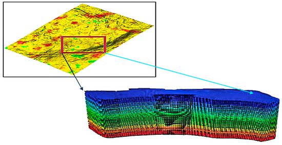
Figure 7.
Numerical model from geo-model.
2.2.2. Gas–Water Relative Permeability in Pore Scale
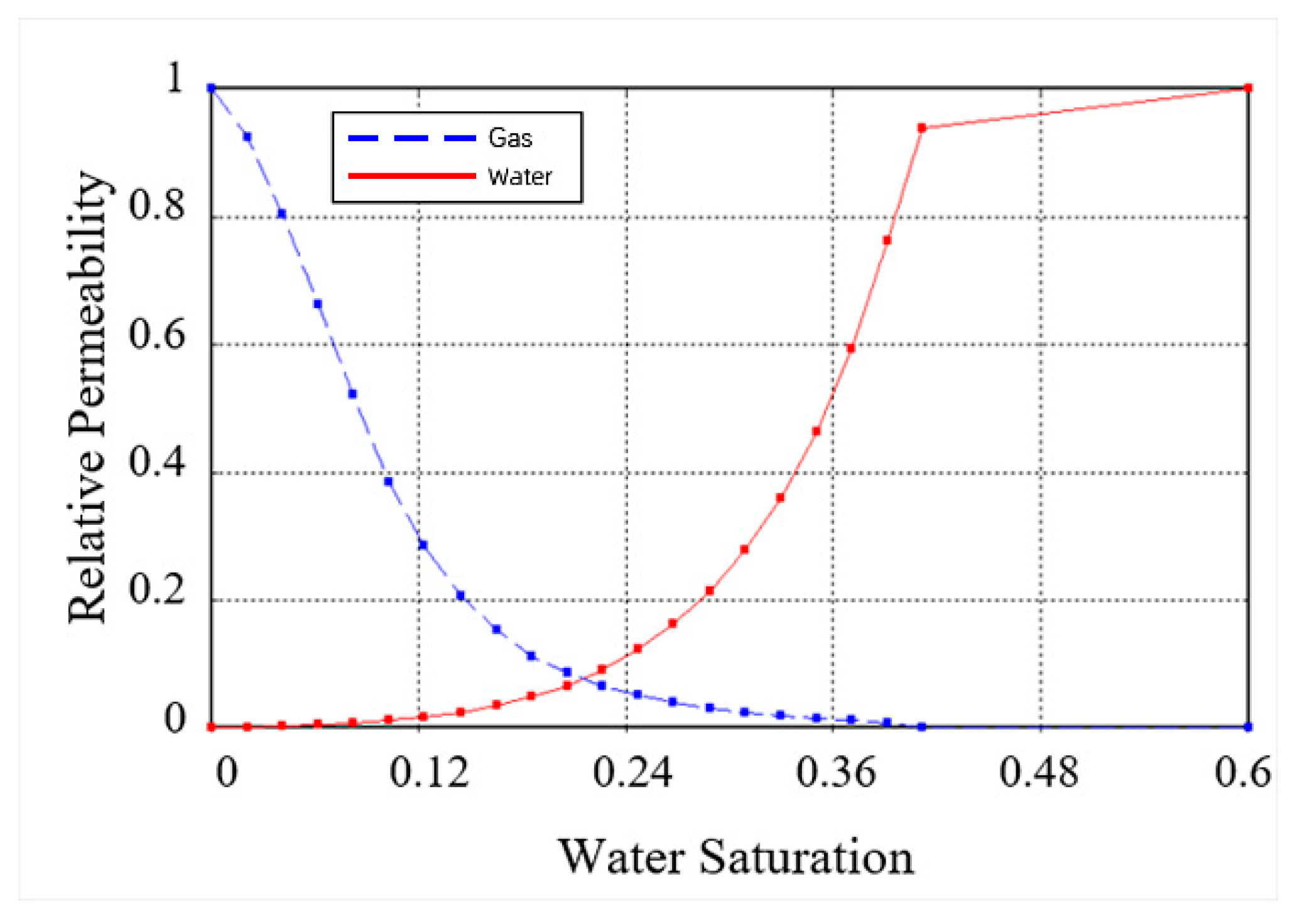
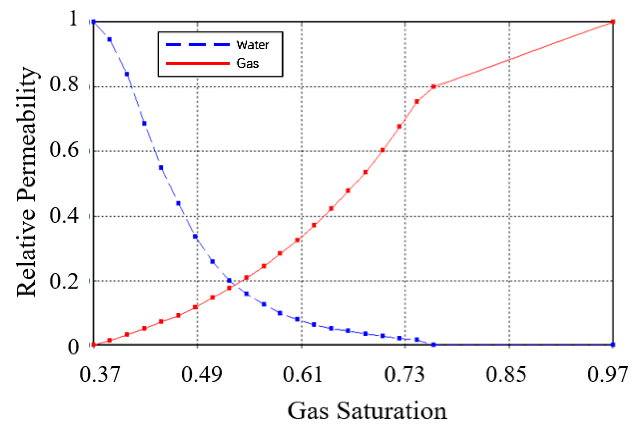
On the left side of the isotonic point, relative permeability increased quickly as water saturation increased; on the left side, relative permeability increased swiftly as water saturation decreased (Figure 8). Water filled both the large and small pores in the reservoir as gas started to enter. Because coal is highly hydrophilic, the gas first selected big pores as the preferred channel to break through. Following the breakthrough, under the displacement pressure, the relative permeability of the gas rapidly rose. The overall water relative permeability dropped when gas replaced the water in the reservoir, showing a trend that first appeared to occur slowly and then quickly Figure 8. Furthermore, demonstrating coal’s significant hydrophilicity is the greater water saturation at the isotonic point. Understanding capillary and gas–water relative permeability at the pore scale has direct implications for reservoir performance. It influences production strategies.
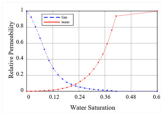
Figure 8.
Relative permeability of water.
The isotonic point gradually moved to the right as the confining pressure increased, and the relative permeability of the water clearly reduced. In contrast, the relative permeability of the gas somewhat increased (Figure 9). When the water saturation was less than 80%, the relative permeability ratio (krg/krw) increased with the increase in the confining pressure. This suggests that the influence of the confining pressure increase on the relative permeability of gas was less than that on the relative permeability of water [17]. The formation water settled in smaller pores and the area surrounding pore throats as the cleat aperture shrank due to an increase in confining pressure. Nonetheless, in low permeability media, the Klinkenberg effect can increase the apparent gas permeability by orders of magnitude [18], partially offsetting the reduction in gas permeability brought on by stress compression (the permeability measured by flowing gas is always greater than the permeability obtained when a liquid is the flowing fluid, and there is almost no difference of the gas molecular velocities in the porous media between the walls and center). The relative permeability of each phase (gas and water) is a function of phase saturation.
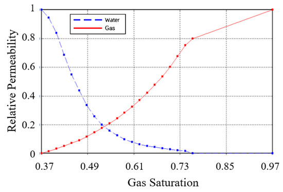
Figure 9.
Relative permeability of gas.
This characteristic reflects the history of fluid displacement and saturation within the pore spaces. Gas and water relative permeabilities are not single-valued functions and can differ for drainage (displacing water with gas) and imbibition (displacing gas with water) processes. Pore-scale modeling and simulations, such as Lattice Boltzmann Modeling (LBM) or pore-network modeling, help in understanding the flow behaviors based on the physical properties measured through imaging. The findings at the pore scale can be up-scaled to understand and predict the macroscopic flow behaviors of the reservoir, which is essential for effective petroleum production and subsurface engineering projects. Through such an analysis, one can understand the interplay of forces acting at the microscopic level and how they govern the efficiency of processes, such as enhanced oil recovery or water flooding, in reservoir engineering.
2.2.3. Model Data Processing
- (1)
- Dynamic data processing
In the process of history matching, the gas production volume, injection gas volume, and other data of each well are given according to the actual production data of the block. When performing history matching, these data are adjusted to make the numerical model more accurate, and also provide the ability to handle data that changes in real time or near-real time. It refers to systems that can adjust to varying loads of information, can update their processes accordingly, and can often incorporate live input from different sources. Consequent adjustments to these datasets are fundamental to refining the numerical model’s fidelity, thereby enhancing the model’s capacity for adapting to real time or near-real time data flux.
- (2)
- Collection and use of well history data
Well history data can reflect the production status of a well. Well history data mainly include data information, such as perforation, refilling, and layer plugging. These data times are treated in the same way as production data times. The depth of these data must be compared and corrected according to the division of small layers to ensure that the layers are consistent with the actual reservoir.
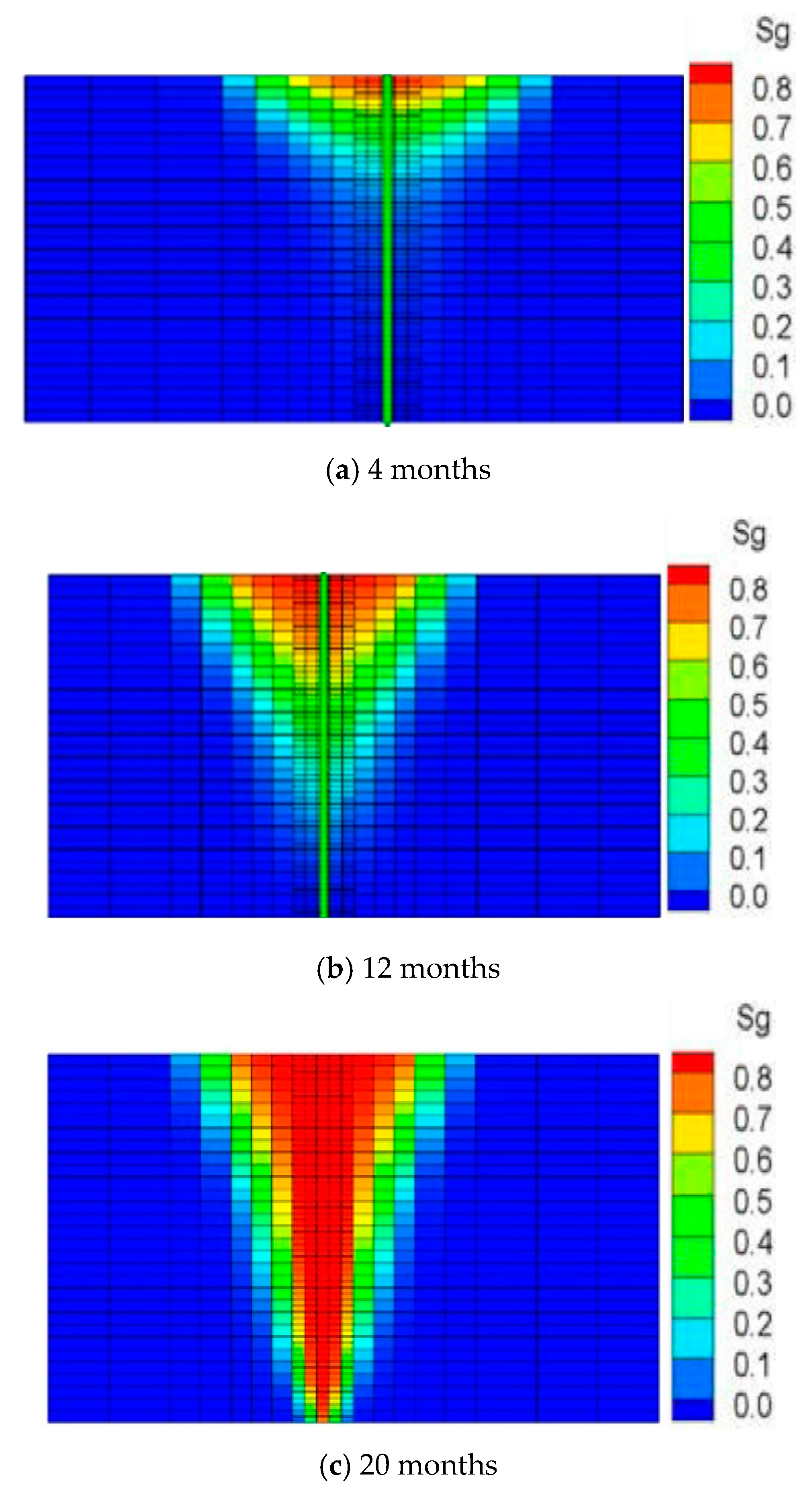
Figure 10a is intended to depict the initial stages of the gas injection procedure. Specifically, it would elucidate the early positioning of the gas plume within the aquifer. During this nascent phase, the gas plume is expected to reside relatively close to the surface, resulting in a limited footprint atop the water-saturated porous rock stratum. This depiction underscores the preliminary spatial distribution of the injected gas within the underground Jia’er gas reservoir.

Figure 10.
Influences of time on gas saturation.
Figure 10b now shows the gas plume expanding within the aquifer, with an increased footprint indicating more significant displacement of the water brine. Annotations might indicate the average pressure increase within the reservoir and any adjustments made to the injection rate.
Figure 10c shows the gas plume reaching a larger extent, occupying a substantial part of the intended storage space. Possible signs of pressure equalization within the reservoir could be shown, with gas beginning to spread laterally. Considerations for maintaining the integrity of the cap rock and ensuring the effectiveness of the seal could be noted, such as continuous monitoring for any leakage or pressure anomalies. The injection slows down as it nears the desired operational capacity to manage pressures carefully and avoid fracturing the cap rock.
2.3. Production History Matching
2.3.1. Determine the Reservoir Production Working System
In the process of production history matching, the first step involved was determining the reservoir production working system. Once the reservoir geological model was established, meticulous history matching ensued, focusing on the development process of the target block. This rigorous matching aimed to replicate the production history of the simulation area since its inception. A critical aspect of this endeavor was determining the injection volume of all injection wells. This step is pivotal in ensuring the accuracy and fidelity of the simulation, as it directly influences the behavior of the reservoir and its production dynamics. By meticulously calibrating injection volumes, the model can better reflect the real-world conditions and provide invaluable insights for reservoir management and optimization strategies.
2.3.2. Region-Wide History Matching
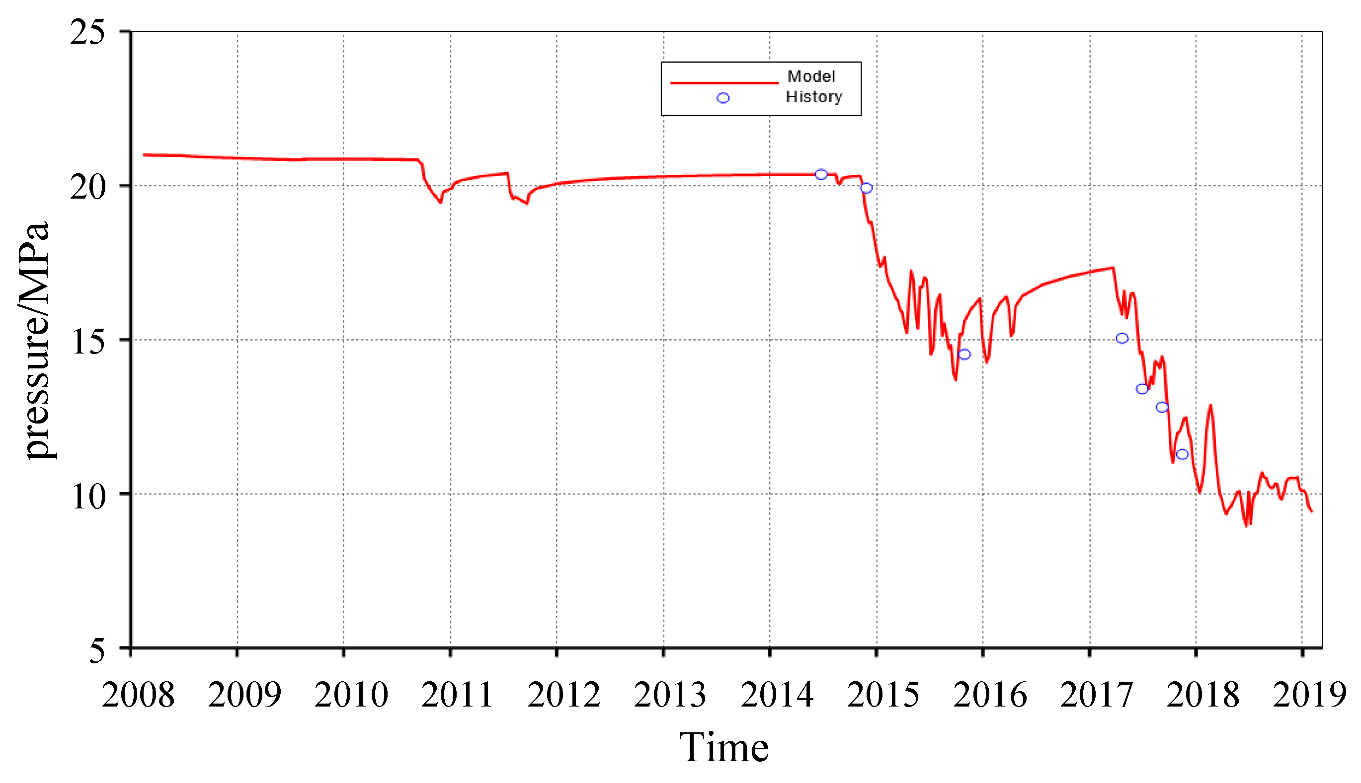
Production data were provided in a range from 2008 to 2019. In order to ensure the accuracy of the reservoir numerical simulation results, the well history data were fully utilized in the history matching process and these data were applied to the numerical simulation model. The overall index fitting mainly considers the following aspects. The geological reserves, reservoir pressure, and comprehensive water content are consistent with the actual formation data, indicating a high fitting (Figure 11, Figure 12 and Figure 13).
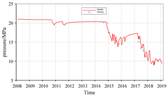
Figure 11.
History matching of gas pressure at datum depth, well W-3.
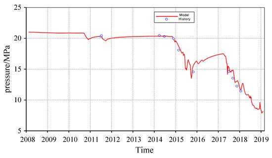
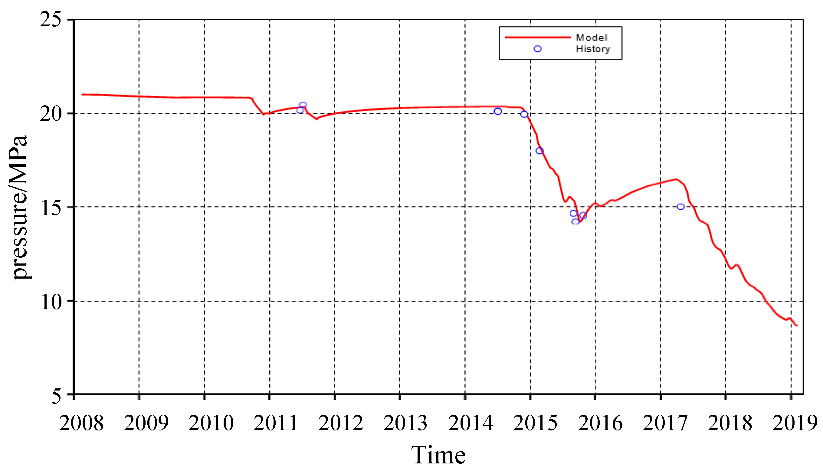
Figure 12.
History matching of gas pressure at datum depth, well W-2.
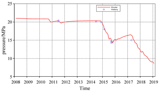
Figure 13.
History matching of gas pressure at datum depth, well W-1.
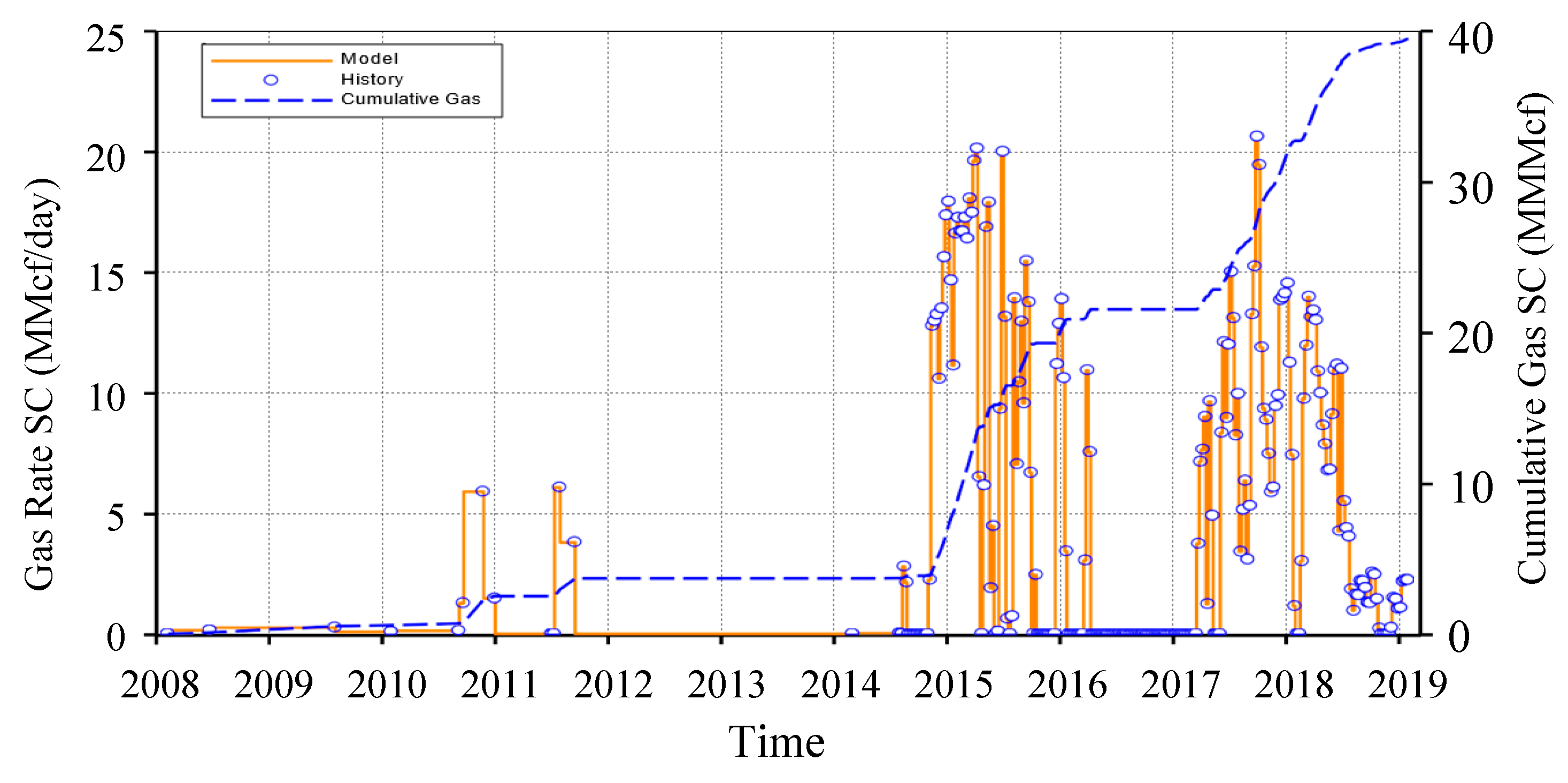
Production prediction is the last step in the Qianjiang field development studies. The aim is to define the Jia’er reservoir production performance under different production scenarios and also find the ultimate recovery for economical estimates of the project costs [19]. The production prediction program is dependent on the size of the Qianjiang field, and the significance of the project and timing may differ from few days to many months. In this study, a production prediction with the aim of depletion to 16.5 MPa (injection pressure), defining the best production strategy, was commenced. The depletion scenario considered is as follows: drilling three new vertical wells, bringing them to production with former producers for fast depletion of the reservoir, and consequently commencing gas injection. In any production scenario there are usually some limitations, which must be considered for production predictions. In this scenario, the following limitations were imposed on each well: (1) maximum production rate from each well, (2) maximum BHP, and (3) produced Water–Gas Ratio (WGR) (Figure 14, Figure 15 and Figure 16).

Figure 14.
History matching of gas production rate, well W-3.
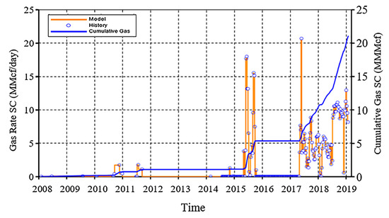
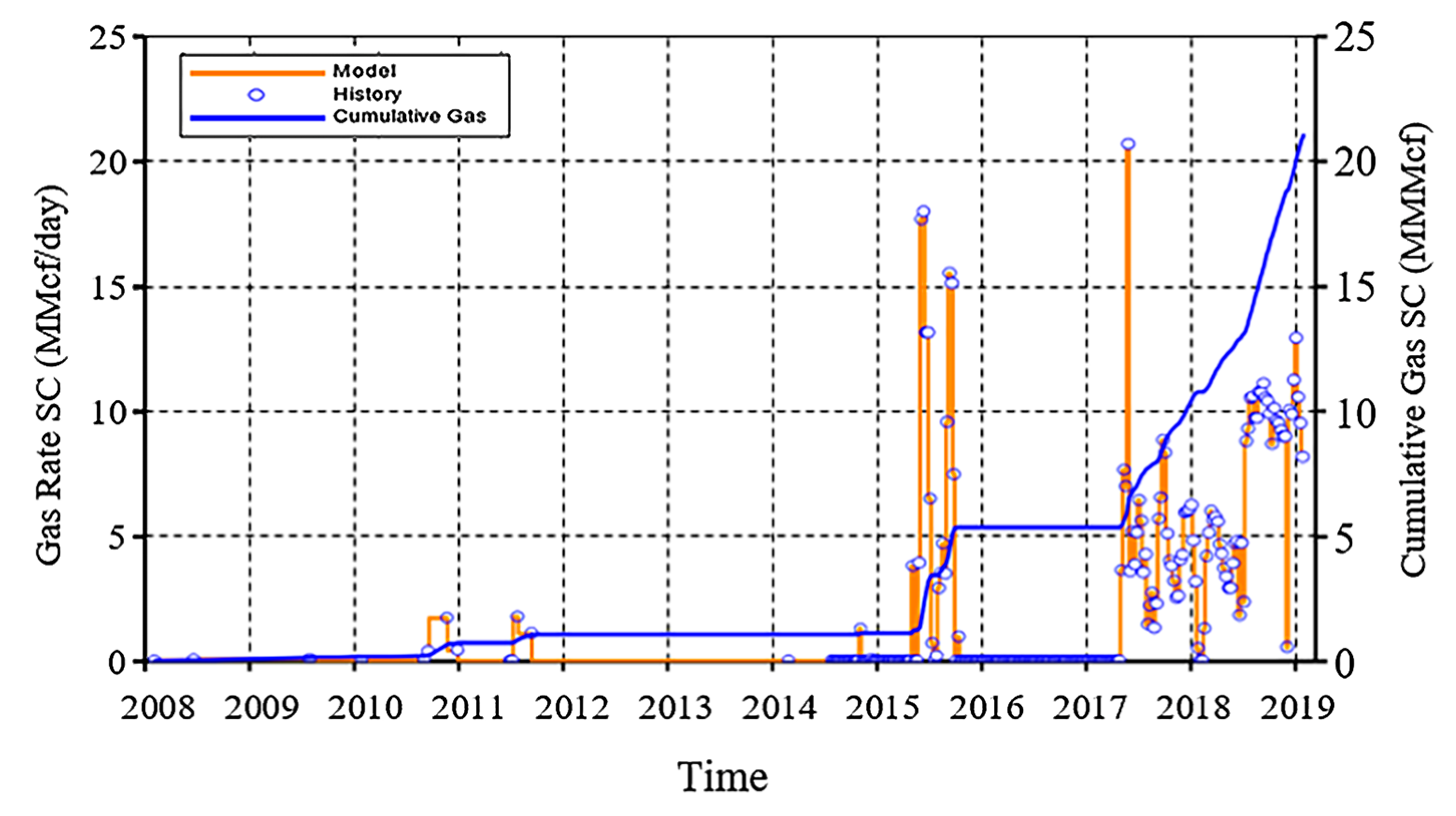
Figure 15.
History matching of gas production rate, well W-2.

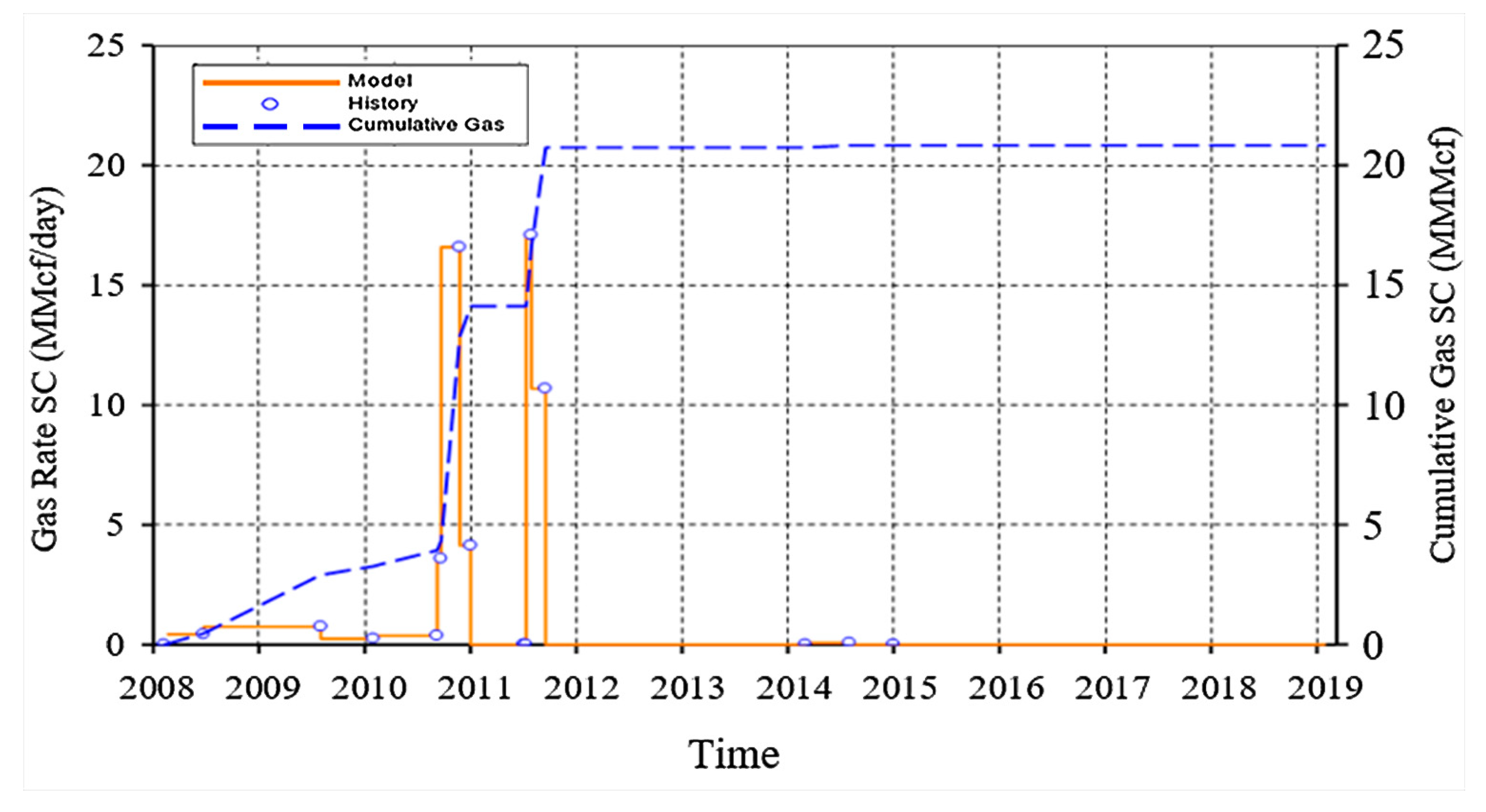
Figure 16.
History matching of gas production rate, well W-1.
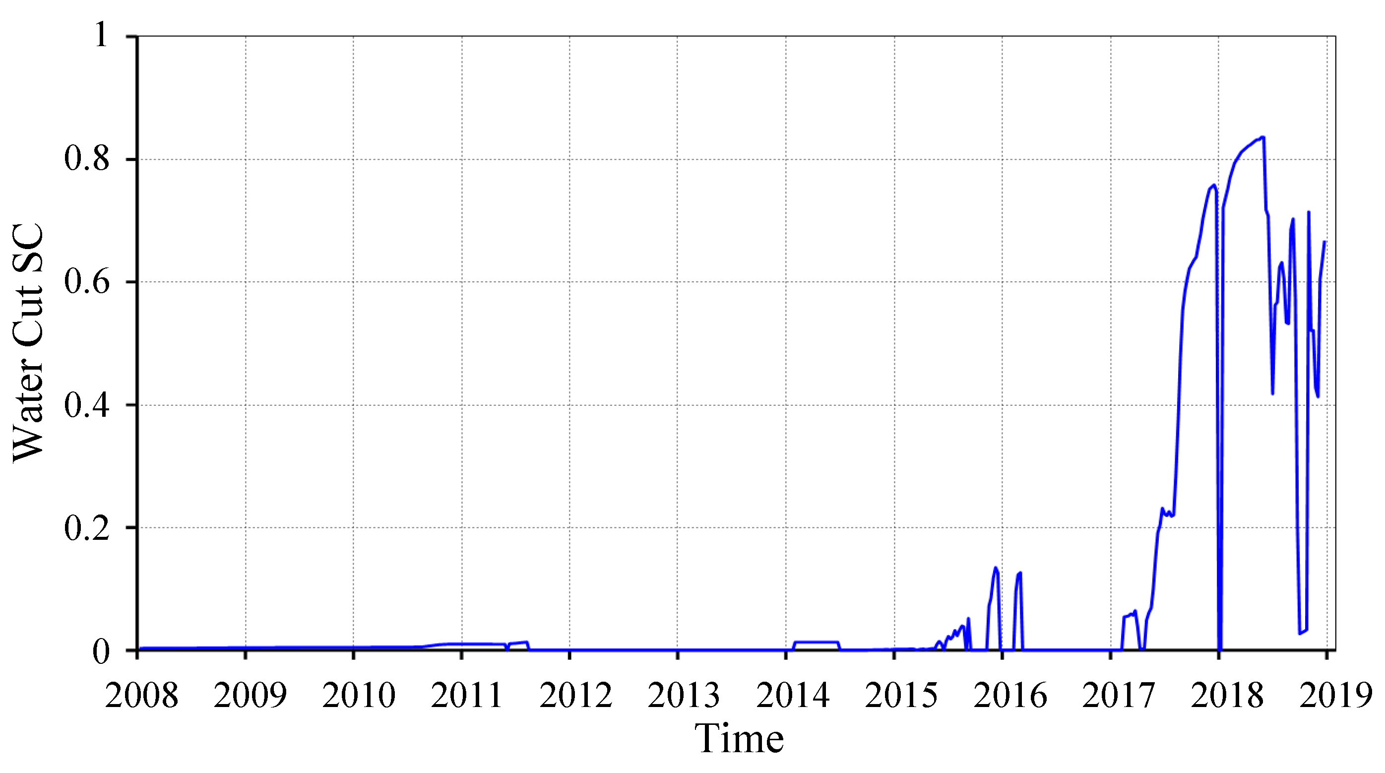
Based on the data depicted in Figure 17, the onset of a water cut can be observed in 2015, with a subsequent increase to 0.12. This trend reversed in 2016, displaying a decrease. However, in 2017, there was a notable resurgence, with the water cut reaching 0.82, maintaining a consistent level through the conclusion of 2018. These fluctuations in water cut levels offer valuable insights into the reservoir’s fluid dynamics and production behavior over the specified time period, shedding light on factors influencing production performance and guiding future reservoir management strategies [20]. Such a detailed analysis contributes to a comprehensive understanding of the reservoir’s behavior and aids in optimizing production operations for enhanced performance and sustainability. These findings underscore the importance of monitoring and analyzing water cut trends to effectively manage reservoir performance and maximize hydrocarbon recovery.
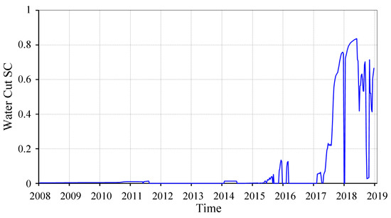
Figure 17.
Water cut.
2.3.3. Single-Well Index Fitting
Taking one month as a time step, from 2008 to 2019, historical matching was performed on all wells using fixed gas production. The fitting included the water cut, oil production, and other factors. After fitting, when the water cut error is less than 10%, the single-well water cut fitting rate reaches 90%. By numerically simulating a single well, the injection–production correspondence between wells was clarified.
2.4. Injection and Production Cycles
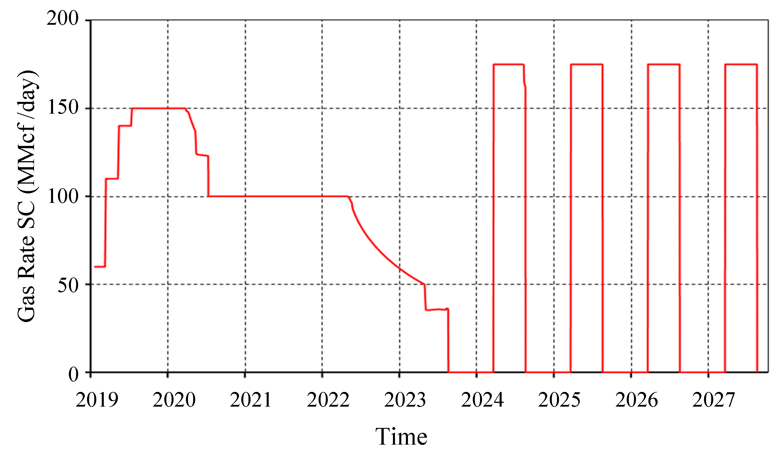
A gas injection rate of 160 MMSCF per day for injection cycles and a production rate of 175 MMCSF per day for production cycles were selected. Injection cycles lasted for 6 months during the hot season and production cycles lasted for 5 months during the cold season. In injection cycles, the maximum injection rate in each well was 40 MMSCF per day and the maximum BHP was set to 23.5 MPa. In production cycles, the maximum production rate in each well was 50 MMSCF per day. In the first cycle, gas injection commenced in early April 2024 and production commenced in early December 2024 and these cycles were repeated for four cycles.
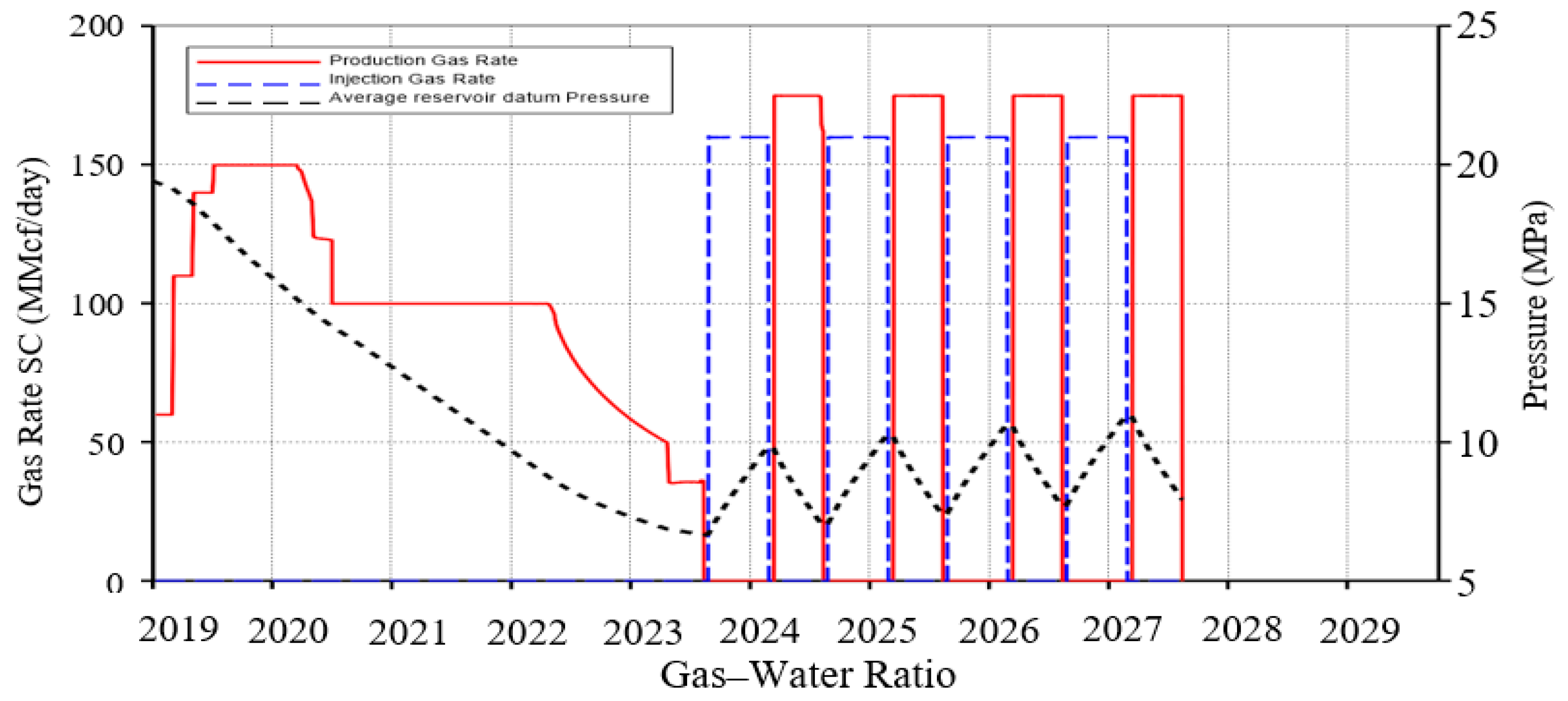
Figure 18 elucidates the filed gas production rate dynamics throughout depletion and production cycles. This figure provides crucial insights into the behavior of gas production over time within the studied Qianjiang field. Additionally, Figure 19 presents a comprehensive depiction of the fluctuations in the average pressure in the Qianjiang field under various scenarios, including depletion, production, and injection cycles. These figures serve as essential visual aids in understanding the performance and behavior of the Qianjiang field under different operational conditions. They offer valuable information for optimizing production strategies and managing reservoir depletion effectively.
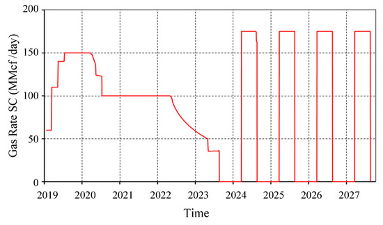
Figure 18.
Gas production–injection cycles.

Figure 19.
Average pressure and production–injection cycles in Qianjiang field.
2.5. Analysis of Cap Rock Safety and Reliability Engineering
2.5.1. Determination of Confidence Interval of Formation Parameters
The safety and reliability of the capping layer at the well site following the reconstruction of the gas storage reservoir in this block were examined using interval theory and the non-probabilistic reliability analysis method, which are based on the logging data of the gas storage reservoir.
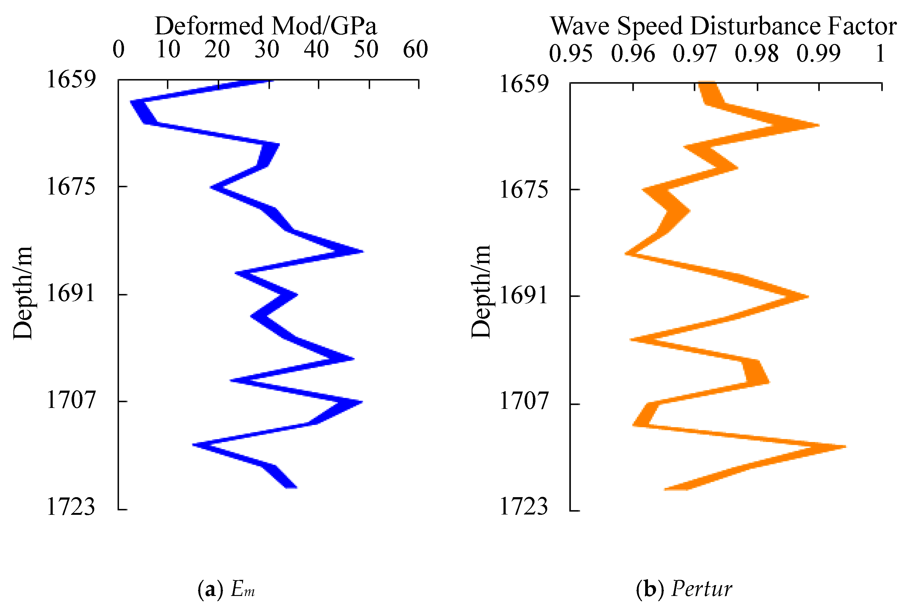
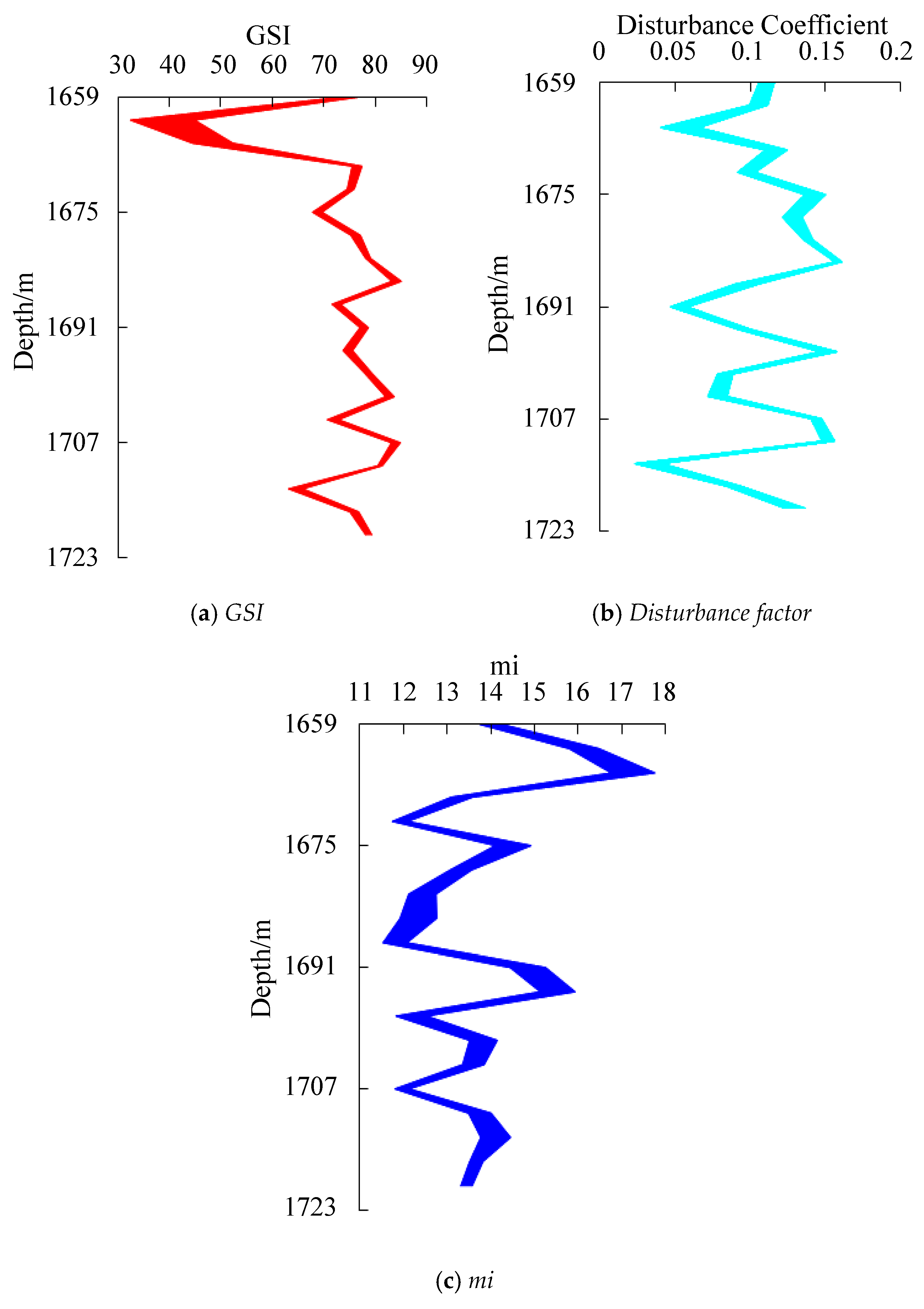
In Figure 20, the variation in the capping layer’s deformation modulus and wave velocity perturbation factor with well depth, as well as the confidence intervals for the deformation modulus and wave velocity perturbation factor, were obtained using the provided logging data along with the error margins of the logging data [21]. By utilizing the interval algorithm and the aforementioned calculation techniques, one can determine the confidence intervals of the geostrength index (GSI) and perturbation factor D based on the deformation modulus and wave velocity perturbation factor. Additionally, the properties of the rock body can be utilized to estimate the confidence intervals of [22,23], as shown in Figure 21.

Figure 20.
Confidence interval of Em and perturbation factor of wave velocity.
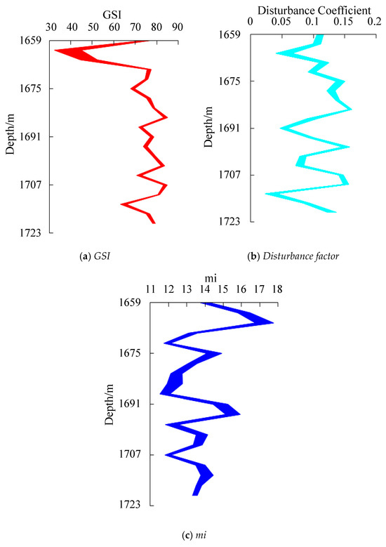
Figure 21.
Confidence interval of GSI, D, and mi.
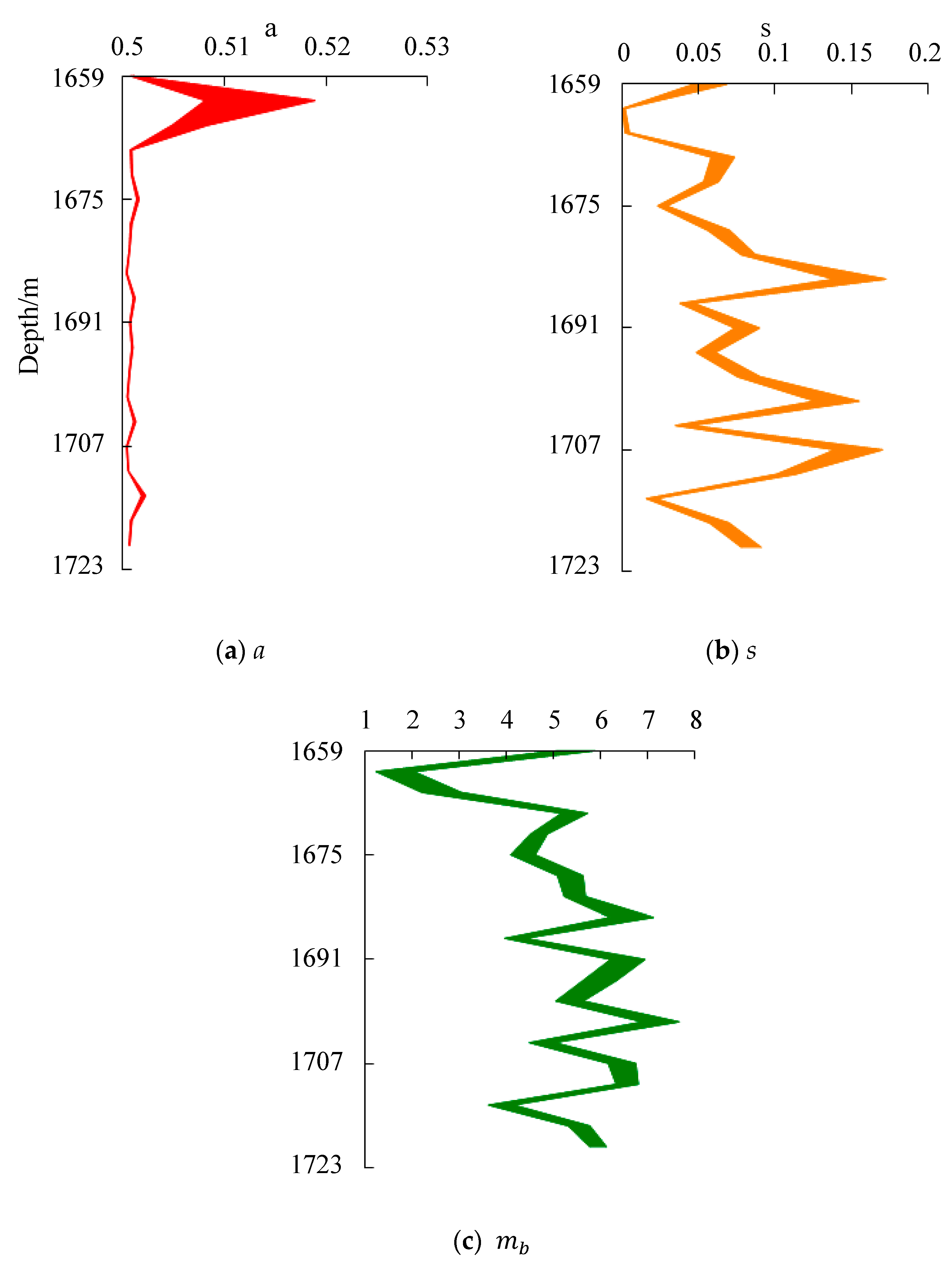
The Hoek–Brown rock mass parameters a, s, and can be calculated (Figure 22) based on the confidence intervals of the cover parameters provided in Figure 21. The picture illustrates how highly varied the confidence intervals are for the rock mass parameters s and , while the parameter a exhibits very little fluctuation outside of a few sites.
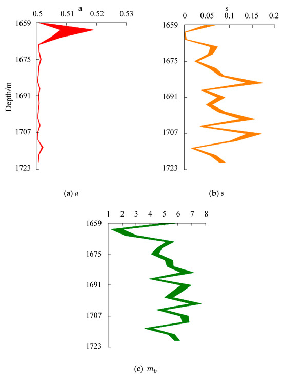
Figure 22.
Confidence interval of a, s, and mb.
Therefore, for the convenience of calculation, the influence of the change in a value can be ignored, and the actual calculation takes a = 0.5. Since s and are monotonous functions of c and ϕ, the interval combination method can be utilized. According to the Hoek–Brown rock parameters, the confidence intervals of the Mohr–Coulomb damage criterion parameters c and ϕ can be obtained.
2.5.2. Analysis of Safety and Reliability of Capping Layer After Gas Injection
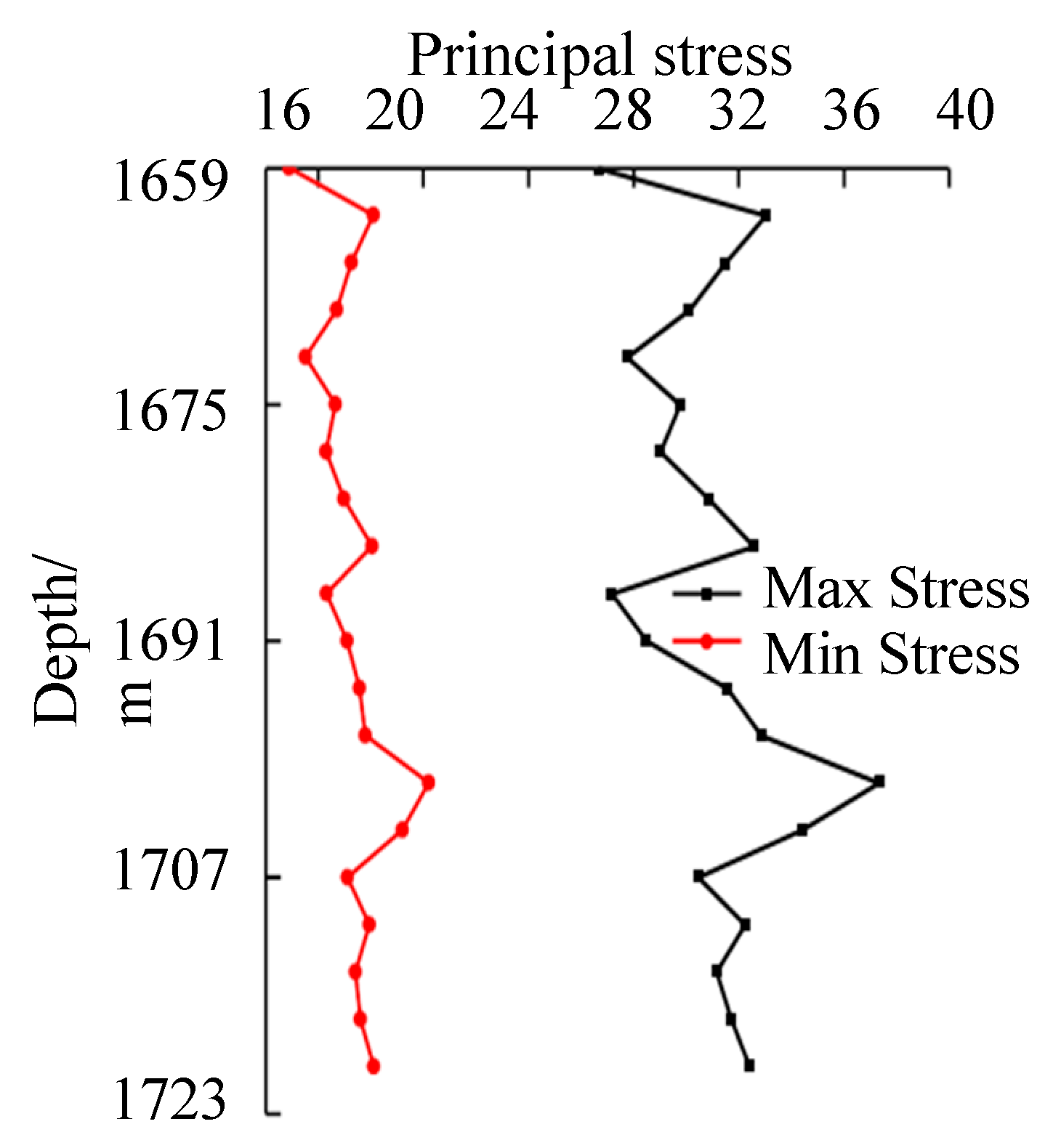
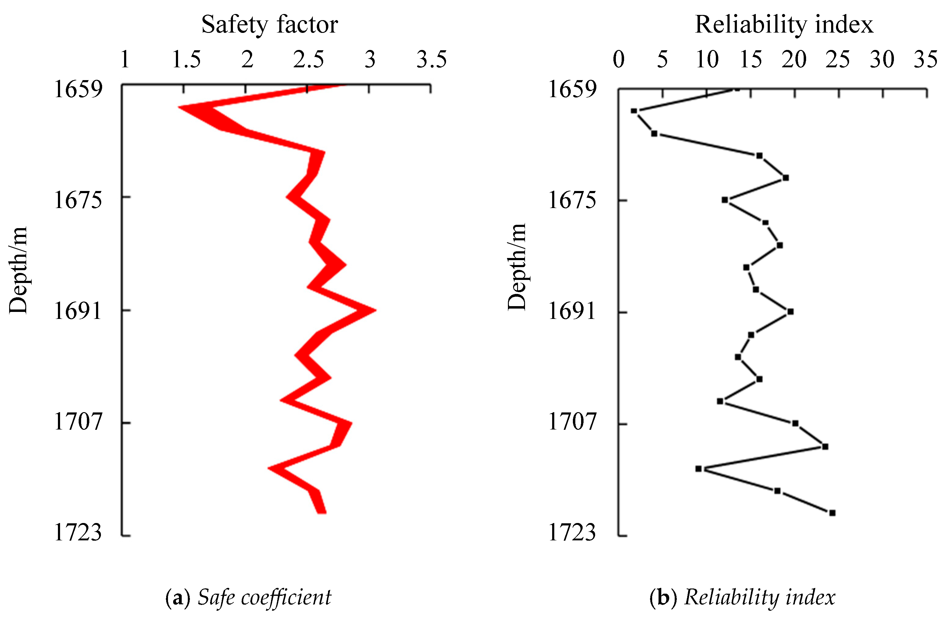
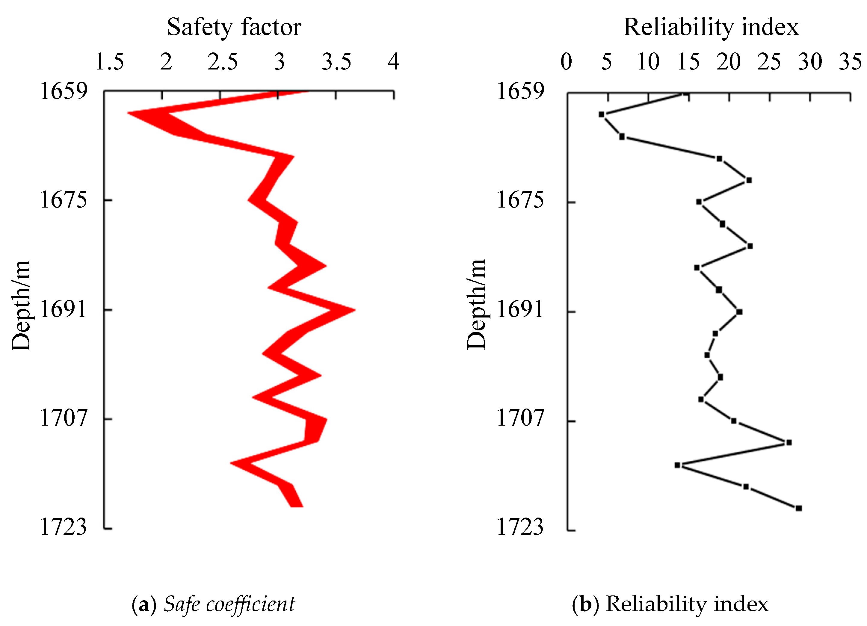
Analyzing the safety and reliability of a capping layer after gas injection involves assessing the structural integrity, containment capabilities, and potential risks associated with the process. According to the logging data, the principal stress of the cap rock was obtained as shown in Figure 23, and as shown in Figure 24 and Figure 25, The minimum safety factor confidence interval and reliability index calculated by the Hoek–Brown failure criterion and Mohr–Coulomb failure criterion for the cover layer are located at a depth of 1665.31 m, with corresponding safety factor confidence intervals of [1.710, 1.460] and [2.035, 1.709], and reliability indices of −3.215 and −0.773, respectively. By comparing Figure 24 and Figure 25, it can be seen that the confidence interval and reliability index of the safety factor calculated by the Hoek–Brown failure criterion are smaller than those calculated by the Mohr–Coulomb failure criterion. The confidence intervals for the safety factor of the cover layer at a depth of 1665.3 m calculated by the Mohr–Coulomb failure criterion are [1.792, 2.010], [2.104, 2.383], and the reliability indicators are −0.909 and 1.744, respectively. Therefore, using the Hoek–Brown failure criterion to calculate the cover layer at a depth of 1665.3 m is unreliable, while using the Mohr–Coulomb failure criterion to calculate the cover layer at that location is reliable. Therefore, the calculation obtained by the Hoek–Brown failure criterion is biased towards safety and conservatism.

Figure 23.
Crustal stress cap rock.
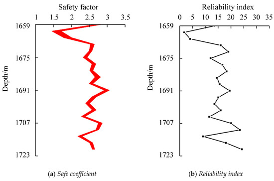
Figure 24.
Safe coefficient and reliability index calculated by Hoek–Brown criterion.
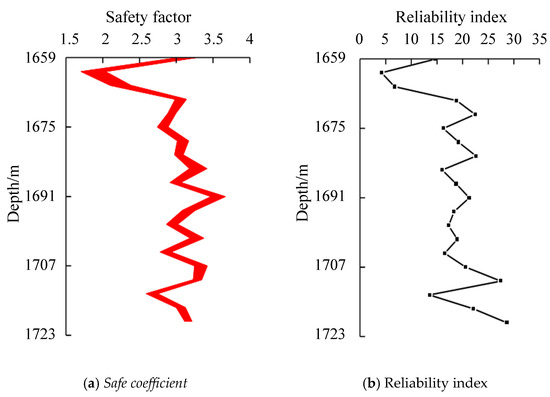
Figure 25.
Safe coefficient and reliability index calculated by Mohr–Coulomb criterion.
2.5.3. Example Analysis
Figure 26 presents the recorded data for the density, natural gamma, and longitudinal wave time difference within the formation depths ranging from 1660 to 1804 m. These readings were extracted from the actual logging curve of the AGS W-3 well located in a gas storage reservoir. These logging measurements provide valuable insights into the composition and properties of the reservoir formation [24]. The recorded values in these figures serve as essential inputs for further geological modeling and reservoir simulation studies.
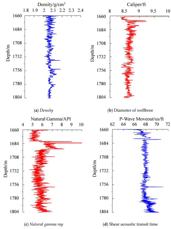
Figure 26.
Logging data of AGS W-3.
In Figure 27, the logging curve data extracted from AGS W-3 well offer a basis for calculating the ground stress and rock mechanical properties. These essential parameters are crucial in understanding the stability and behavior of the rock formation surrounding the well. By utilizing theoretical approaches, researchers can derive valuable insights into the stress distribution and mechanical characteristics, such as the elastic modulus and rock strength [25]. This information is vital for assessing the reservoir’s structural integrity, predicting potential instability issues, and informing drilling and completion design. The logging curve data serves as a valuable tool in the calculation process, enabling accurate characterization of the rock mechanics and supporting safe and efficient operations in the AGS W-3 well and its associated gas storage reservoir. The results obtained from these calculations form a foundation for further analysis and evaluation of the subsurface conditions and reservoir performance.
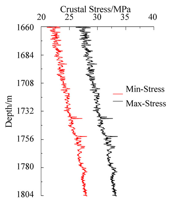
Figure 27.
Crustal stres near the W-3.
The computation findings at 1772 m of the AGS W-3 well were compared and examined with the outcomes of the on-site fracturing test and the on-site pressure results in order to confirm the accuracy of the results. This comparison demonstrated a strong correlation between the simulation results and the practical test outcomes.
2.6. Analysis of Maximum Operating Pressure of Gas Storage
2.6.1. Uncertainty Analysis of Rock Mass Parameters
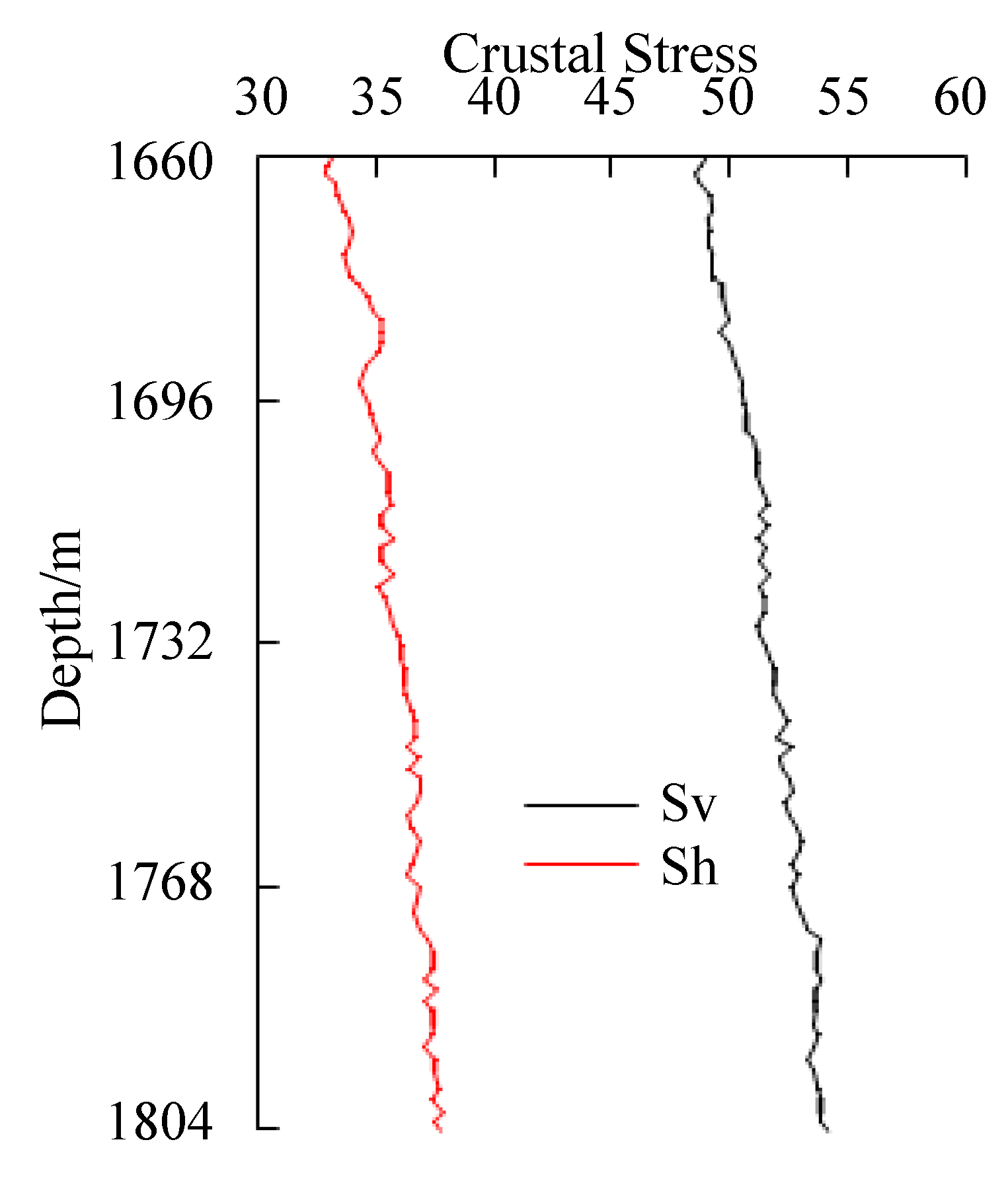
The confidence interval of the maximum operating pressure and the risk factor of the inactive faults were analyzed using interval theory based on the well logging data of a domestic aquifer following the reconstruction of the aquifer into a gas storage reservoir [26]. According to the geological data and reservoir information, the angle θ between the direction of the inactive fault and the direction of minimum principal stress in the reservoir area is 61.32°, the initial pore pressure is 15.1 MPa, and the pore pressure after gas injection is 20.32 MPa.
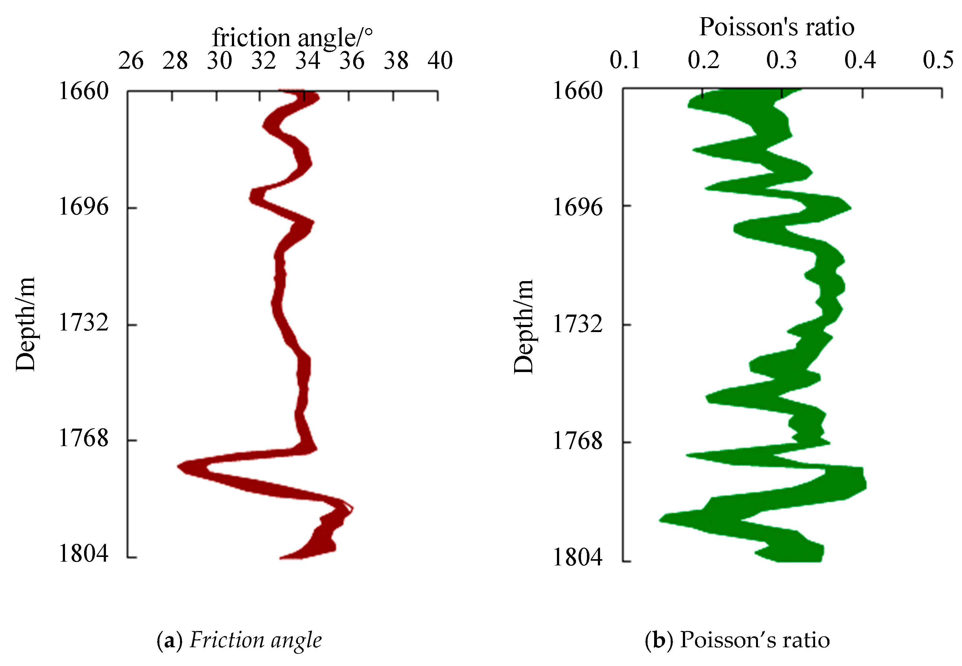
Based on the confidence ranges of the transverse and longitudinal wave timing disparities that were derived from the analysis of various well logging data sets, representative locations were taken (Figure 28), and the geostress situation at the fault site can be seen in Figure 29.

Figure 28.
Confidence interval of friction angle and Poisson’s ratio.

Figure 29.
Crustal stress near the fault.
The confidence interval of the rock body’s internal friction angle and Poisson’s ratio were determined using the interval algorithm [27,28]. It is evident that the range of values for the internal friction angle confidence interval is clearly smaller than that of the Poisson’s ratio confidence interval. This is based on the confidence interval of the transverse wave time difference and longitudinal wave time difference [29]. As an illustration, the largest fluctuation in the confidence interval of the internal friction angle occurs at 1775.3 m, and the confidence interval of the internal friction angle is [28.25, 29.48], with a difference of 4.2% between the maximum value and the minimum value, while the largest fluctuation in the Poisson’s ratio occurs at 1678.2 m, and the Poisson’s ratio has a confidence interval of [0.18, 0.28]. Given a 35.7% discrepancy between the highest and minimum values, this suggests that while the beginning parameter is not the most significant, its value is different. This phenomenon, which shows a 35.7% correlation, suggests that the initial parameter uncertainty has a larger impact on the Poisson’s ratio.
2.6.2. Determination of Maximum Operating Pressure
Based on the well logging data, the confidence interval of the fault hazard factor was determined after gas injection to the location of the inactive fault. This will yield the confidence interval of the geostress and rock mass parameters on the fault, as shown in Figure 30.
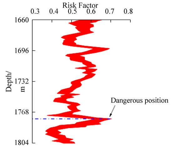
Figure 30.
Confidence interval of risk coefficient.
To calculate a confidence interval for a risk coefficient, you typically need three pieces of information: the point estimate of the risk coefficient (e.g., from a regression analysis), the standard error of the estimate, and the desired level of confidence. The hazard coefficient of the fault obtained by interval theory has a large fluctuation range due to the consideration of parameter uncertainty, as can be seen from the confidence interval of the hazard coefficient given in Figure 30. The largest hazard coefficient occurs at the location of 1775.3 m, and the confidence interval of the hazard coefficient at this location is [0.61, 0.69], indicating that under the current conditions of parameter uncertainty, all of the hazard coefficient values in this interval are conceivable, with the bottom and upper limit values being 0.61 and 0.69, respectively. This indicates that the author considers this position to be the most dangerous location of the inactive fault due to the uncertainty around the existing parameters. The riskiest location was then used to examine the confidence interval of the gas storage reservoir’s maximum operational pressure, as shown in Figure 31. The confidence intervals for the maximum operating pressure determined using single-parameter mean value calculations and interval theory are displayed in Figure 31. As the pore pressure at the most dangerous location of the fault rises, the risk factor also rises, and the fault is in a state of critical damage when the risk factor is used, and the corresponding pore pressure can be considered as the maximum operating pressure of the gas storage reservoir. The maximum operating pressure that can be obtained by using the mean value of a single parameter is 24.3 MPa, which is located in the maximum operating pressure confidence interval, according to Figure 31. However, the calculation’s maximum operating pressure is greater than the lower bound of the maximum operating pressure’s confidence interval when the parameters are uncertain [30]. The procedure for determining the maximum operating pressure of a system is a critical aspect of ensuring safe and efficient functionality. This involves a set of calculations and tests that take into account the material properties, design limits, environmental factors, and stress loads the system is expected to endure. By establishing the upper limit of pressure that a system can safely withstand, engineers can prevent structural failures and ensure compliance with relevant safety standards and regulations. Moreover, this threshold helps in designing operating procedures that maximize the system’s performance while minimizing the risk of overpressure incidents. Continuous monitoring is often employed to ensure that the actual pressures remain well within the defined safe operating limits. This could potentially affect the underground gas storage reservoir on the inactive fault’s ability to operate safely. Therefore, the maximum operating pressure of the underground gas storage reservoir can be chosen to be the lower limit of the confidence interval of the maximum operating pressure in order to guarantee the safety of the reservoir, i.e., 23.5 MPa is taken as the maximum operating pressure of the reservoir, and the pore pressure at the location of the inactive fault in the process of gas injection should not exceed this value.
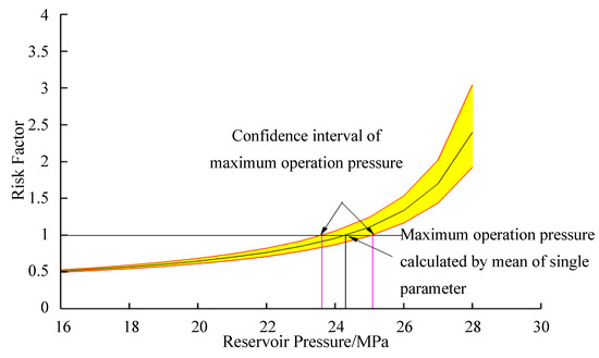
Figure 31.
Confidence interval of maximum operating pressure.
3. Conclusions
This paper analyzes the main problems in injection and production, including underground gas storage and the maximum operating pressure of gas storage, along with the reliability of reservoirs and potential faults. Corresponding solutions are provided, providing theoretical references and guidance for the construction and safe operation of aquifers in Qianjiang field. The main research conclusions and prospects obtained in this article are as follows:
- (1)
- Modeling of Aquifer Type Trap and Seepage Mechanism
① Geo-modelling and numerical simulation techniques have emerged as a pivotal approach in comprehensively understanding and effectively managing underground natural gas storage in aquifer reservoirs. Through the intricate integration of geological data interpretation, reservoir characterization, and fluid flow simulation, we have constructed robust reservoir models that encapsulate the complex geological heterogeneity and fluid behavior inherent in aquifer systems.
② According to the data at hand and the model generated by CMG2022 software, Qianjiang field exhibits potential as a suitable candidate for underground gas storage (AGS) implementation. Once the aquifer reservoir is around 23.5 MPa, a gas injection cycle featuring an injection rate of 160 MMSCF per day and a subsequent gas production cycle at 175 MMSCF per day can be initiated. Moreover, it is imperative to drill additional production wells to facilitate the necessary pressure reductions within the reservoir and ensure a delivery capacity of 150 MMSCF per day, inclusive of production from the existing three gas producer wells.
- (2)
- Prediction of Maximum Operating Pressure of Aquifer Gas Storage Reservoirs
① Considering the influence of the uncertainty in rock parameters on the failure of inactive faults, the confidence interval of the fault danger coefficient after gas injection was obtained using logging data and interval theory. Based on the confidence interval of fault danger coefficient, the maximum operating pressure for fault stability in gas storage was obtained.
② Using the method described in this article, the confidence interval and maximum operating pressure of the fault danger coefficient of a certain aquifer gas storage reservoir in Qianjiang field were analyzed. The analysis results showed that as the dip angle of the fault increased, the fault danger coefficient first increased and then decreased. When the dip angle of the fault is θ, and the friction angle with rock is φ, the relationship is , and the fault has the highest risk factor and is the most prone to breaking. The confidence interval for the maximum hazard coefficient of the gas storage fault obtained is [0.61, 0.69], and the maximum operating pressure of the gas storage is 23.5 MPa.
③ The maximum operating pressure of a gas storage facility that was calculated using interval theory and considering parameter uncertainty is smaller than the result obtained without considering parameter uncertainty. Therefore, to ensure the safe operation of the gas storage facility, the lower limit of the confidence interval for the maximum operating pressure can be selected as the maximum operating pressure of the gas storage facility.
- (3)
- Non-Probabilistic Reliability Analysis of Aquifer Reservoir Cover and Faults
① Based on the characteristics of shear failure in potential faults, the convex set theory was introduced into the non-probabilistic reliability analysis of potential faults. The limit state function for the reliability analysis of potential faults was established, and coordinate transformation was performed on the obtained limit state function during its calculation process to simplify its calculation. When analyzing the reliability of the model, it is not necessary to obtain the probability distribution function of the sample and large-scale sample sampling is not necessary.
② This method was used to study the potential fault reliability of an underground gas storage facility in Qianjiang field after gas injection. The calculation results of this method were compared with those of the Monte Carlo method. The maximum error between the reliability obtained in this thesis and the reliability obtained from the Monte Carlo calculation was 11.1%, which can meet the accuracy requirements of engineering calculations.
③ As the uneven coefficients of geostress and pore pressure increase at potential fault locations, the reliability of the slip of potential faults decreases. The reliability of the slip of potential faults varies with their dip angle θ, which first decreases and then increases. When θ is related to φ, the relationship is as follows: . At this time, the reliability of the potential fault slip is low.
Author Contributions
Y.X.: Conceptualization, Methodology, Investigation, Software, Validation, Writing—original draft. Z.S.: Conceptualization, Data curation, Validation, Supervision, Funding acquisition, Writing—review and editing. W.C. and R.W.: Supervision, Resources. B.Y. and J.L.: Methodology, Software. Z.R. and Y.W.: Writing—review and editing. C.G.: Visualization. Y.J.: Visualization. All authors have read and agreed to the published version of the manuscript.
Funding
This research received no external funding.
Data Availability Statement
The data presented in this study are available on request from the corresponding author.
Conflicts of Interest
Authors Wei Chen, Beibei Yu, and Jiqin Liu were employed by PipeChina Engineering Technology Innovation Co., Ltd. Author Zhongxin Ren was employed by National Pipeline Network Group Energy Storage Technology Co., Ltd. Author Ruidong Wu was employed by CNOOC China Ltd. Author Yufeng Jiang was employed by CNOOC Energy Development Co., Ltd. The remaining authors declare that the research was conducted in the absence of any commercial or financial relationships that could be construed as a potential conflict of interest.
References
- Li, B.; Chen, X.X.; Yang, Q.Y. The Fundamentality of Construction Underground Gas Storage to Solve the Imbalance of Gas Consumption. Oil Gas Storage Transp. 2013, 22, 7–10. [Google Scholar] [CrossRef]
- Wang, Y. Application and Development of Natural Gas Underground Storage Facilities. Pet. Storage Gas Stn. 2008, 4, 23–26. [Google Scholar]
- He, C.; Xia, H.N.; Xia, W. The Current Situation of China’s Underground Gas Storage. Equip. Manuf. Technol. 2013, 8, 246–247. [Google Scholar]
- Ding, G.S.; Xie, P. Current Situation and Prospect of Chinese Underground Natural Gas Storage. Nat. Gas. Ind. 2006, 6, 111–113. [Google Scholar]
- Tarkowski, R.; Uliasz-Misiak, B.; Tarkowski, P. Storage of hydrogen, natural gas, and carbon dioxide—Geological and legal conditions. Int. J. Hydrogen Energy 2021, 46, 20010–20022. [Google Scholar] [CrossRef]
- Fan, Z.W. Global natural gas development pattern and the analysis of development direction of natural gas in China. China Min. 2018, 27, 11–16. [Google Scholar]
- Zhang, G.X.; Li, B.; Zheng, D.W. Challenges to and proposals for underground gas storage (UGS) business in China. Nat. Gas Ind. 2017, 37, 153–159. [Google Scholar] [CrossRef]
- Tan, Y.F.; Lian, L.M.; Yan, M.Q. The Technology and Development of Foreign Underground Natural Gas Storage. Oil Gas Storage Transp. 1997, 16, 17–19. [Google Scholar]
- Zhan, C.H.; Jiao, W.L.; Lian, L.M. Underground Gas Storage Reservoir Constructed in Water-Beating Formation. Nat. Gas Ind. 2001, 21, 88–91. [Google Scholar]
- Ding, G.S. Developing trend and motives for global underground gas storage. Nat. Gas Ind. 2010, 30, 59–61. [Google Scholar] [CrossRef]
- Wei, H.; Tian, J.; Li, J.Z. The current situation and development trend of underground natural gas storage facilities in China. Int. Pet. Econ. 2015, 23, 57–62. [Google Scholar]
- Zhang, F.Q.; Zeng, P.; Zhou, L.J. Underground Gas Storage Research Status Quo and Application Expectations at Home and Abroad. China Coal Geol. 2021, 33, 39–42+52. [Google Scholar] [CrossRef]
- Liu, H.Y. Opportunities and challenges of underground natural gas storage based on carbon peak and carbon neutrality goals. Pet. Nat. Gas Chem. Ind. 2022, 51, 70–76. [Google Scholar] [CrossRef]
- Zeng, D.Q.; Zhang, J.F.; Zhang, G.Q. Research progress of Sinopec’s key underground gas storage construction technologies. Nat. Gas Ind. 2020, 40, 115–123. [Google Scholar]
- Xu, J.J.; Wang, Q.J.; Xu, M. Dynamic characteristics of underground gas storage rebuilt from carbonate gas reservoir with bottom water and the water flooding mechanism of its well. Oil Gas Storage Transp. 2019, 38, 5227. [Google Scholar] [CrossRef]
- Wang, Y.F. The Development Prospects of Aquifer Gas Storage Construction in China. Pet. Knowl. 2023, 3, 38–39. [Google Scholar]
- Li, J.C.; Shen, R.C.; Yuan, G.J.; Qu, P.; Gao, Y.B. Research of Relative Construction Technology about Aquifer Gas Storage. Oil Gas Storage Transp. 2009, 28, 9–12. [Google Scholar] [CrossRef]
- Yekta, A.E.; Manceau, J.C.; Gaboreau, S.; Pichavant, M.; Audigane, P. Determination of hydrogen–water relative permeability and capillary pressure in sandstone: Application to underground hydrogen injection in sedimentary formations. Porous Media 2018, 122, 333–356. [Google Scholar] [CrossRef]
- Basso, O.; Lascourreges, J.F.; Le, B.F. Characterization by culture and molecular analysis of the microbial diversity of a deep subsurface gas storage aquifer. Res. Microbiol. 2017, 160, 107–116. [Google Scholar] [CrossRef]
- Rutqvist, J.; Birkholzer, J.; Cappa, F. Estimating maximum sustainable injection pressure during geological sequestration of CO2 using coupled fluid flow and geomechanical fault-slip analysis. Energy Convers. Manag. 2019, 48, 1798–1807. [Google Scholar] [CrossRef]
- Xu, H.C.; Zhang, S.J.; Li, X. A new design method of minimum storage pressure of underground gas storage rebuilt from gas reservoir. Nat. Gas Geosci. 2020, 31, 1648–1653. [Google Scholar]
- Zheng, Y.L.; Sun, J.C.; Qiu, X.S. Connotation and evaluation technique of geological integrity of UGSs in oil-gas fields. Nat. Gas Ind. 2020, 40, 4103. [Google Scholar] [CrossRef]
- Ding, G.S.; Wei, H. Review on 20 years’ UGS construction in China and the prospect. Oil Gas Storage Transp. 2020, 39, 2531. [Google Scholar] [CrossRef]
- Wang, T.T. Research on the Deformation Rules and Safety of Surrounding Rock of Gas Storage in Multi-Layered Salt Rock Mass; China University of Petroleum: Beijing, China, 2016. [Google Scholar]
- Ding, G.S.; Li, X.B.; Jiang, F.G. Discussion on Emergency Gas Supply and Peak Shaving of the Second West to East Gas Pipeline. Nat. Gas Ind. 2008, 12, 92–94. [Google Scholar]
- Yu, B.F.; Yan, X.Z.; Yang, H.L. Non-probabilistic reliability analysis of dead fault slip in underground gas storage based on convex model. J. Pet. Sin. 2014, 35, 577–583. [Google Scholar]
- Zhao, G.F. Engineering Structure Reliability Theory and Application; Dalian University of Technology Press: Dalian, China, 1996. [Google Scholar]
- You, L.J.; Sha, J.X.; Gao, X.P. Simulation Tests of Effective Stress Changes in Gas Storage during Injection and Production. Pet. Drill. Tech. 2020, 48, 1048. [Google Scholar]
- Wang, C.H.; Gao, G.Y.; Jia, J. Variation of stress field and fault slip tendency induced by injection and production in the H underground gas storage. Nat. Gas Ind. 2020, 40, 7685. [Google Scholar] [CrossRef]
- Federico, G. The Spanish Gas and Electricity Sector: Regulation, Markets and Environmental Policies; IESE Business School, Universidad de Navarra: Barcelona, Spain, 2018. [Google Scholar] [CrossRef]


Disclaimer/Publisher’s Note: The statements, opinions and data contained in all publications are solely those of the individual author(s) and contributor(s) and not of MDPI and/or the editor(s). MDPI and/or the editor(s) disclaim responsibility for any injury to people or property resulting from any ideas, methods, instructions or products referred to in the content. |
© 2025 by the authors. Licensee MDPI, Basel, Switzerland. This article is an open access article distributed under the terms and conditions of the Creative Commons Attribution (CC BY) license (https://creativecommons.org/licenses/by/4.0/).