1. Introduction
With the continuous advancement of technology and the profound restructuring of global industries, the static mixer industry is faced with unprecedented market opportunities [
1,
2,
3,
4,
5]. These devices play a vital role in various fields, such as marine industries, nuclear power, and renewable energy, due to their advantages in regard to enhancing mixing efficiency, reducing energy consumption, and improving operational stability [
6,
7,
8,
9,
10]. The working principle of a static mixer is that under the influence of high-pressure, high-speed conditions, the fluid medium is guided by fixed mechanical components to carry out the mixing process of different fluids, as shown in
Figure 1. This process involves physical phenomena, such as strong shear, backflow, and wall impacts, and it involves a nonlinear dynamics problem [
11,
12,
13,
14,
15,
16]. Therefore, the design optimization of static mixers focuses more on fluid dynamics and multifunctional integration. Advances in intelligent design have made it possible for static mixers to adjust their internal structures according to the fluid characteristics and process requirements to achieve optimal mixing results. For example, with regard to chemical enhancement processes, after the addition of mixing blades or perforated plates, the fluid exhibits dynamic characteristics, such as splitting, stretching, and collision, which lead to the complex and nonlinear evolution of the mixing flow field. This results in phenomena like shock-induced vibrations and noise and impacts the performance and service life of static mixers [
17,
18,
19,
20,
21,
22]. Therefore, the study of the mixing transport properties of the two-phase flow in static mixers and design optimization strategies involving complex component structures has significant engineering application prospects for enhancing the overall performance of static mixers.
In the above engineering applications, the mixer’s flow field becomes complex due to the guidance and shear effects of the mixing blades. The characteristic parameters of the flow field are influenced by various factors, including the geometric dimensions of the mixing pipeline, internal component design, and flow field distribution. Non-moving elements, such as blades or corrugated plates, alter the trajectory of the fluid flow. In contrast, spiral mixing elements and baffle blades induce local acceleration and directional changes in the fluid. This results in the decomposition of the fluid velocity into three components and the formation of a hierarchical flow field. These mixing actions primarily facilitate distributed mixing through convection. However, when distributed mixing reaches an advanced level, diffusion enhances the mixing uniformity at the molecular scale. Therefore, it has significant scientific research value to conduct an in-depth study of the dynamic characteristics of static mixers, to explore the mixing flow and diffusion mechanisms, and to determine the optimal values for the key flow field parameters [
23,
24].
As a new type of industrial equipment, static mixers are replacing traditional dynamic mixers, such as batch stirrers and Venturi tubes, due to their extensive application potential. Researchers are investigating the mixing mechanisms of static mixers and are striving to enhance their overall performance. Haddadi et al. used the Reynolds-averaged turbulence model to conduct a comprehensive study of the flow field in static mixers, and their results were highly consistent with the experimental data [
25]. Visser et al. examined the mixing behavior of low-viscosity and high-viscosity fluids in an SMX-type static mixer and found that the calculated wall heat transfer coefficient was slightly lower than the experimental value, due to the failure to consider the heat conduction effect of the mixing blades [
26]. Michael et al. performed numerical studies on an SMX mixer and found that the pressure loss predictions for non-elastic and viscoelastic fluids aligned with the experimental results [
27]. Hosni et al. conducted a detailed analysis of the two-phase flow pressure drop in a Kenics static mixer and developed a new friction factor model to reduce the characteristic mixing time [
28]. Talhaoui et al. employed computational fluid dynamics (CFD) techniques to investigate the mixing behavior of incompressible Newtonian fluids and demonstrate that geometrically optimized static mixers can achieve rapid mixing and enhance mixing quality [
29]. Lebaz et al. studied the dispersion characteristics of oil droplet sizes in static mixers under turbulent conditions and found that the average droplet size increased with the concentration of the dispersed phase but decreased with an increasing main-phase flow rate [
30]. Wang et al. analyzed the symmetric structure of the Kenics static mixer and found that the pressure drop was smaller for the classic symmetric structure [
31]. Zhuang et al. conducted particle image velocimetry experiments and CFD simulations on a double vortex static mixer and achieved high accuracy for pressure loss coefficients [
32]. These studies provide significant theoretical and experimental support for the design optimization and performance enhancement of static mixers.
Current research on static mixers predominantly emphasizes the dynamic modeling of two-phase flow, velocity distribution characteristics, and pressure fluctuations. Most existing studies adopt conventional mesh-based numerical approaches such as Reynolds-averaged turbulence models or finite volume methods. While these techniques have yielded important insights, they often lack the resolution required to accurately capture strong turbulence and nonlinear interface behaviors, especially in complex mixing structures. Despite progress, challenges remain in resolving multiphase interface deformation, transient flow instability, and the interaction of multiple velocity components within geometrically intricate mixers. The internal flow structure often involves high-shear regions, vortex shedding, and dynamic coupling between flexible and rigid mixing elements, resulting in strongly nonlinear fluid behavior. In this context, the simulation approach adopted in this study—based on the lattice Boltzmann method (LBM) coupled with LES turbulence modeling—offers a promising alternative. LBM has inherent advantages in handling transient and complex boundary flows, making it particularly suitable for studying nonlinear two-phase flow dynamics in static mixers. Therefore, the proposed modeling strategy aims to overcome the current limitations and provide a more accurate and robust framework for analyzing multiphase mixing characteristics and guiding structural optimization.
Building upon the identified challenges, this study proposes a comprehensive numerical framework based on the lattice Boltzmann method (LBM) to investigate multi-component velocity mixing dynamics in static mixers. Given the inherent design of static mixers, which induces considerable turbulence and intense shear effects, conventional numerical schemes often suffer from instability or reduced accuracy. To prevent computational divergence due to time discretization and improve stability under strong shear and unsteady flow conditions, the LBM relaxation model is optimized specifically for static mixer applications. Coupled with a large eddy simulation (LES) turbulence model, a two-phase flow model is developed to capture the complex interactions between the fluid and solid boundaries during the mixing process. This framework is then employed to examine the mixing behavior under varying flow velocities and static mixer configurations, aiming to reveal the underlying mechanisms of multiphase mixing. The novelty of this study lies in integrating LBM with local mesh refinement and LES turbulence closure to simulate two-phase mixing in geometrically complex static mixers. Compared with conventional CFD approaches, the proposed method offers superior resolution in capturing shear-dominated structures and nonlinear interface dynamics. As such, it addresses existing modeling limitations and provides a more accurate and robust tool for analyzing multiphase mixing processes and guiding the structural optimization of static mixers.
This paper is organized as follows: In
Section 2, a static micromixer model based on the Lattice Boltzmann Method (LBM) is established, and a hybrid LBM–LES solving method is proposed. In
Section 3, a two-phase flow mixing and transport dynamics model for the static micromixer is constructed.
Section 4 discusses the numerical results and analysis of the flow field variations induced by different inlet velocities and blade angles. In
Section 5, the conclusions are presented.
4. Numerical Results and Discussion
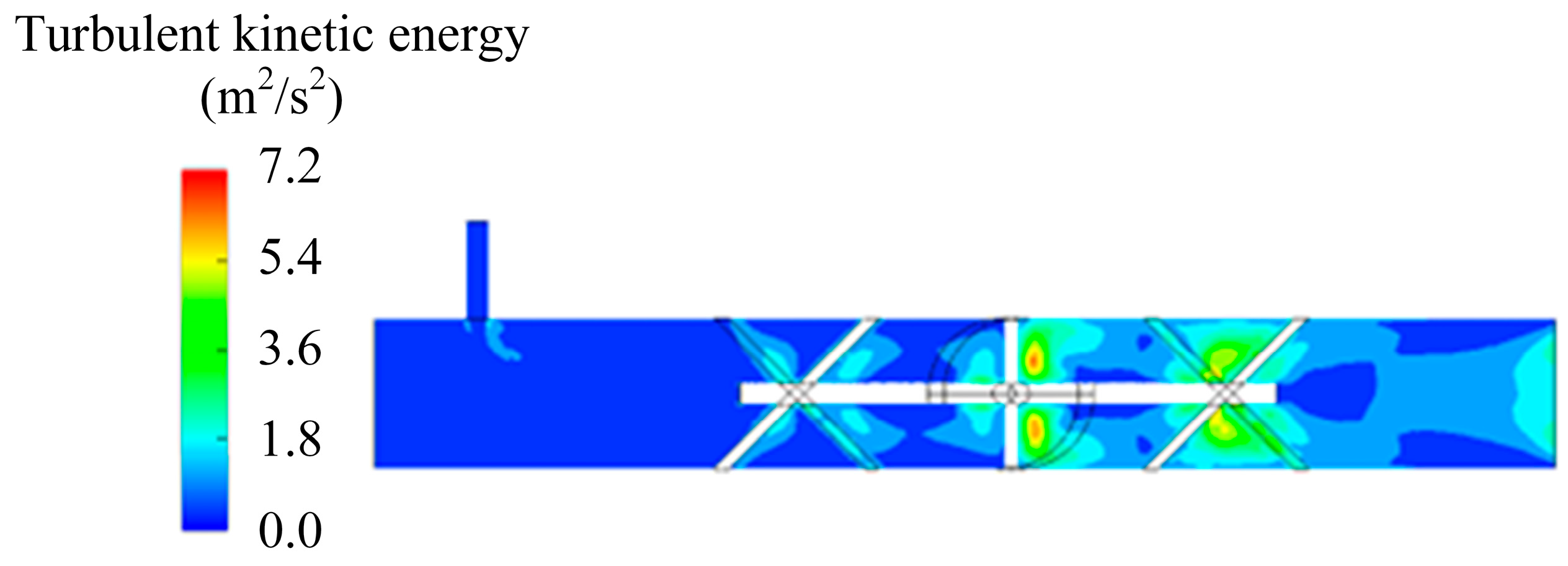
4.1. Evolution Trend of Turbulent Kinetic Energy
Investigating the distribution of turbulent energy can provide insights into the effectiveness of mixing blades, the primary mixing regions, and the relative positions of vortex and turbulent energy increase zones.
Figure 7 shows the distribution of turbulent kinetic energy on the symmetry plane when the inlet speed is 4 m/s. It can be observed that the turbulent kinetic energy is higher around the blades and in the flow after passing through the blades. As the fluid passes through the mixing blades, the turbulent kinetic energy near the blades significantly increases, indicating that the blades enhance the turbulent kinetic energy of the flow field. Combining the analysis of velocity and pressure in the flow through the blades, it can be found that there are low-speed, low-pressure areas behind the blades. The flow direction changes abruptly and making it easier for regions with higher turbulent kinetic energy to form vortices. The presence of vortices helps to promote macroscopic mixing in the flow field. Thus, the blades are the main factor in the mixing process. The turbulent kinetic energy within the static mixer is relatively high, and there are greater opportunities for vortex diffusion and splitting. The role of turbulent diffusion in promoting mixing can be determined by analyzing the turbulent distribution in the region behind the blades.
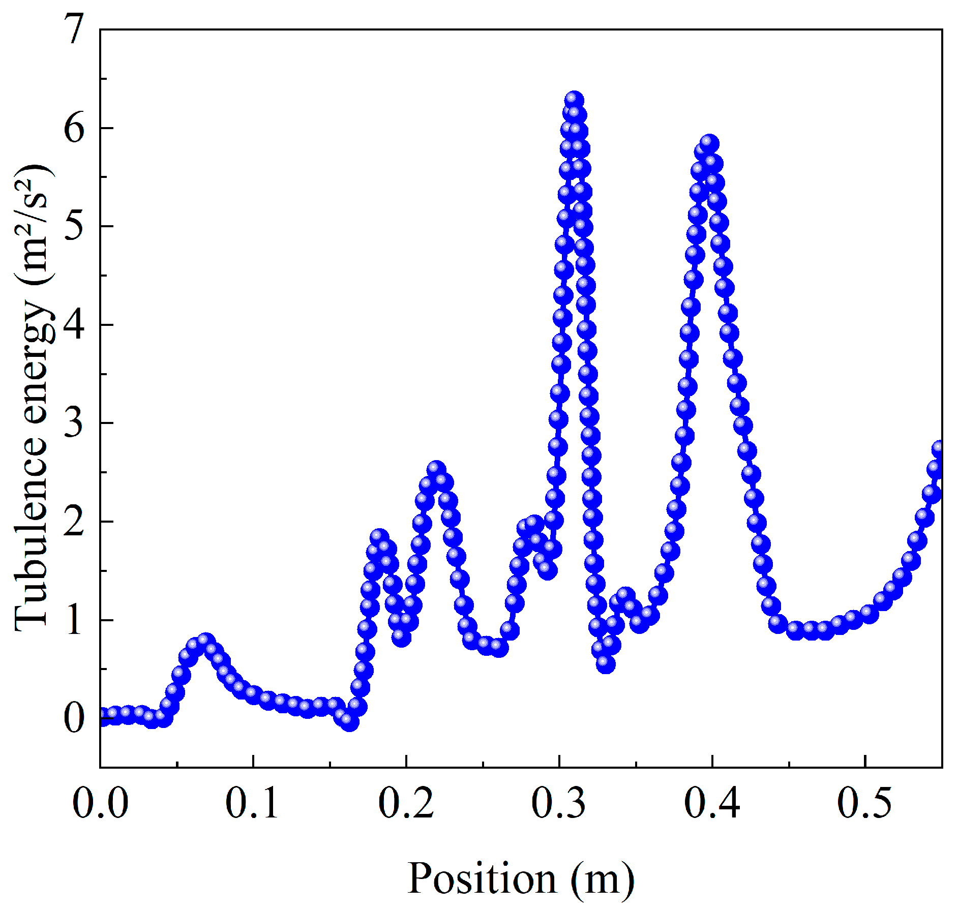
To study the distribution of turbulent kinetic energy in a static mixer, the turbulent kinetic energy located on the axial line at
r = 0.25
d near the wall is chosen, as shown in
Figure 8. The first peak of turbulent kinetic energy is caused by the fluid medium entering the channel from inlet 2. After the fluid medium enters the mixer, under the influence of the main flow velocity in the pipeline, the velocity differentiates into multiple sub-velocities, accompanied by energy consumption, which decreases in total turbulent kinetic energy. As the fluid passes through the first set of blades, due to the guiding effect of the blades, the velocity increases and the turbulent kinetic energy also increases, especially in the wake region behind the blades, and the turbulence intensity of the fluid reaches its peak. Then, the turbulent kinetic energy rapidly decreases with the diffusion of the flow. When passing through the second set of blades, the phenomenon is similar to the first set, and the turbulent kinetic energy reaches its peak again. This process repeats, but the peak of turbulent kinetic energy first increases and then decreases, and it attains its maximum near the second set of blades. The main reason for the increase in peak value is the interaction between the two sets of blades, which leads to the superposition of turbulent kinetic energy, but its value is limited. At the third group of blades, the turbulent kinetic energy decreases. Therefore, the role of the blades is the main reason for the increase in turbulent kinetic energy.
4.2. Effect of Inlet Velocity on the Mixed Pressure Field
A static mixer is a new type of mixing equipment, and its core mechanism is to achieve mixing by increasing the pressure drop in the system. Pressure drop is an important parameter in the design of various new types of static mixers. In addition to its configuration, the factors affecting the pressure drop of a static mixer are also related to its material and the properties of the fluid. Therefore, the pressure drop of the static mixer is influenced by the flow rate and blade angle. Since the pressure varies with the flow rate, this paper describes the pressure variation in a static mixer using the static pressure distribution along the axis.
Figure 9a shows the pressure variation curve within the static mixer at 0.2 s when the inlet 1 velocity is 4 m/s. Before entering the mixing zone, the pressure drop changes slowly, due to the friction between the fluid and the side wall. At this time, the pressure dissipation during the flow process is small, so the pressure drop can be ignored. In the axial direction, the pressure decreases in a stepwise manner, with the main pressure drop occurring after the fluid passes through the blades. In the section from the inlet of the static mixer to the blade area, due to the lower friction coefficient of the pipe wall, the flow resistance is also small, and the static pressure remains nearly unchanged. This low friction can be attributed to the smooth inner surface of the pipe, which reduces wall roughness and suppresses the development of a turbulent boundary layer. Additionally, in this pre-mixing zone, the flow is predominantly laminar or transitional, resulting in weaker viscous shear interactions between the fluid and the wall. As a result, the wall shear stress is relatively low, minimizing energy loss in this region. When fluid encounters the mixing blades, the static pressure exhibits a stepped decline trend. This is due to the obstruction of the blades, energy dissipation, sudden changes in flow direction, rapid increase in turbulent kinetic energy, and the conversion of static pressure into dynamic pressure.
The pressure distribution at a certain cross-section in the middle of three sets of blades has been obtained, as shown in
Figure 9b. From the analysis of the radial cross-section pressure distribution cloud map, it can be seen that the pressure distribution exhibits a stepped pressure drop from the outer side to the inner side at the cross-section. In certain areas of the mixer, especially in front of the blades, high-pressure zones can be observed. This is due to the fluid being compressed before entering the blades, increasing pressure. At the rear of the blade and at the outlet of the mixer, a low-pressure area can be observed. This is due to the expansion and turbulence of the fluid behind the blades, which leads to a decrease in pressure. The fundamental reason is that when the fluid encounters the blades, the difference in shear forces on the inside and outside of the blades causes abrupt changes in flow speed and direction, leading to energy dissipation and pressure changes. At the same time, it is proven that a sudden change in fluid flow direction will lead to pressure loss, which is also a major cause of pressure drop. By analyzing the pressure distribution, the design of the mixer can be optimized to reduce unnecessary energy loss and improve mixing efficiency.
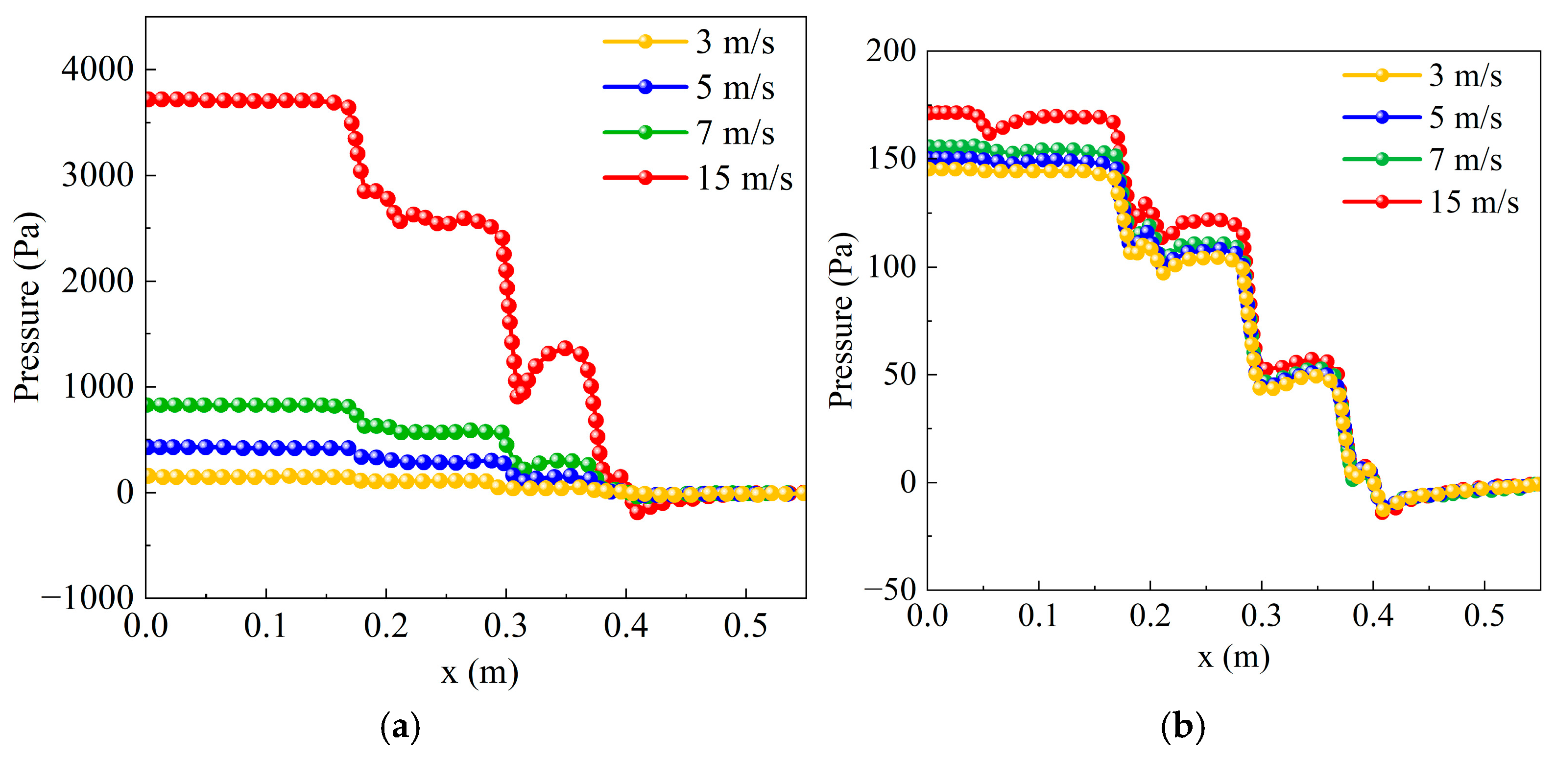
Figure 10 shows the trend of pressure variation along the axis of the static mixer at the near-wall straight section with
r = 0.25
d under different flow rates. In
Figure 10a, it is evident that as the flow velocity increases, the pressure drop near the blades becomes more pronounced. At flow rates of 3 m/s and 5 m/s, the pressure curve remains stable with minor fluctuations, indicating that fluid flow is more consistent at these lower flow rates. The pressure changes are most significant at a flow rate of 15 m/s, with notable pressure fluctuations, particularly between 0.2 m and 0.4 m along the x-axis. This indicates that at higher flow rates, the effects of fluid dynamics become more pronounced, resulting in greater pressure variations. Between 0.35 m and 0.4 m on the
x-axis, a significant low-pressure area appears on the pressure curve at a flow velocity of 15 m/s. This phenomenon is attributed to the fluid encountering increased resistance or expansion from the blades in this region, resulting in a pressure drop.
Figure 10b illustrates the evolution of the pressure drop at inlet 2 across various speeds. The graph reveals that the pressure drop curve exhibits a stepped decline, which is associated with the energy dissipation of the fluid as it interacts with the blades within the mixer. Before the fluid comes into contact with the blades, the pressure drop curve already shows a downward trend. This phenomenon occurs due to the convergence of two fluid streams at the inlet, where the fluid’s viscosity leads to an increase in dynamic pressure and a corresponding decrease in static pressure, resulting in a sudden drop in pressure at the initial position of the axis. As the flow rate at inlet 2 increases, the phenomenon of a sudden initial pressure drop becomes more pronounced. This indicates that the flow rate has a significant impact on pressure drop, with higher flow rates leading to greater energy loss. These observations emphasize that selecting an appropriate flow rate is crucial for the mixing process. A flow rate that is too high may lead to energy waste, while a flow rate that is too low may fail to achieve the desired mixing effect. Therefore, it is necessary to choose a balance point based on the specific application and production requirements of the mixer to achieve the optimal energy efficiency ratio. By optimizing blade design and flow rate, energy consumption can be reduced, achieving energy-saving production. This is of great significance for lowering operating costs and enhancing the competitiveness of enterprises.
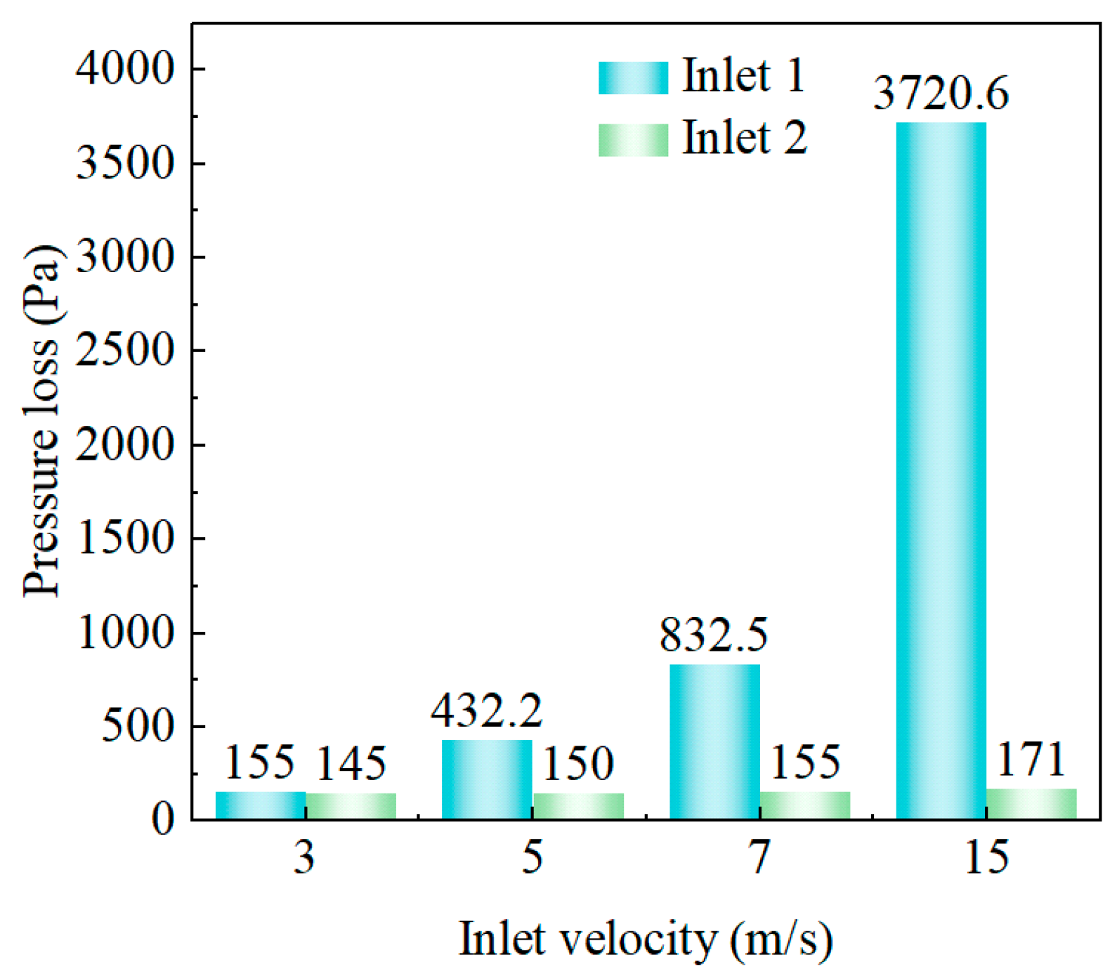
The pressure drop along the axial direction is determined by calculating the static pressure difference between the inlet and outlet along the same axis. An analysis of the data presented in
Figure 11 reveals that variations in the velocity at Inlet 1 significantly influence the pressure drop across the static mixer, while changes in velocity at Inlet 2 have a relatively smaller effect. The results indicate that the pressure drop increases with the flow rate. This increase is attributed to the greater fluid resistance and energy dissipation associated with higher flow rates, particularly near the mixer blades and wall surfaces. When selecting pump power, it is essential to consider both the pressure drop and the mixing performance. An appropriate inlet velocity not only enhances mixing efficiency but also minimizes energy consumption while ensuring the desired output. For instance, if the pressure drop is excessively high, a more powerful pump may be necessary to overcome the resistance, resulting in increased energy usage. Conversely, a very low pressure drop may indicate inadequate mixing performance, which fails to meet the required mixing quality. Therefore, engineers should establish the optimal inlet velocity through experimental studies or numerical simulations when designing and operating static mixers. The ideal inlet velocity achieves a balance between mixing performance and energy efficiency, thereby enhancing production efficiency, lowering operational costs, and contributing to energy savings and emission reductions.
4.3. The Effect of Blade Angle on the Mixed Pressure Field
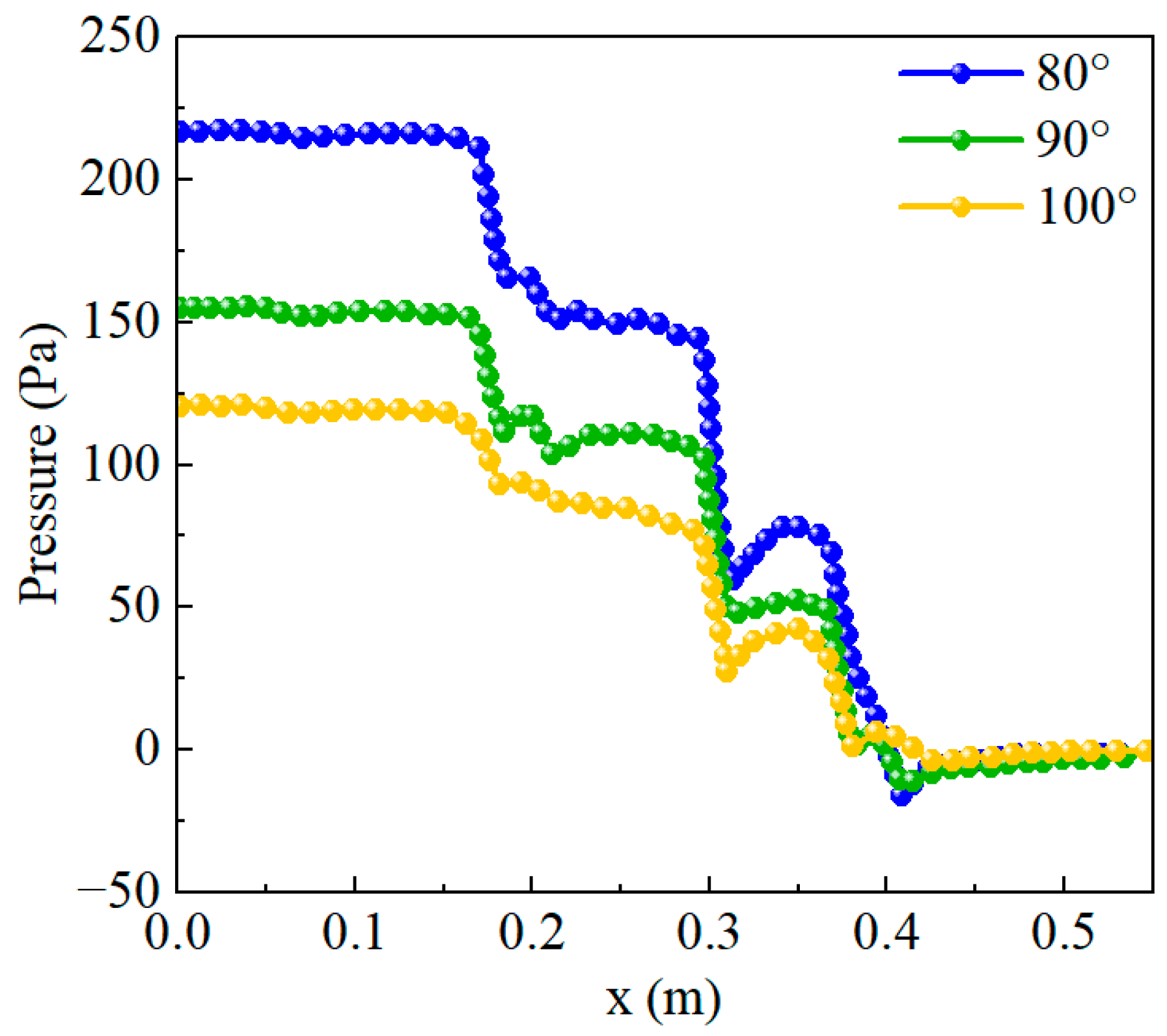
Figure 12 illustrates the pressure drop curves within the static mixer for various blade angle configurations. It is evident that the pressure drop at different blade angles decreases in flow direction, and the trends are similar across the configurations. However, the specific range of pressure changes becomes more pronounced as the blade angle decreases. For instance, the curves corresponding to different blade angles exhibit a significant reduction between 0.2 m and 0.4 m on the
x-axis. This phenomenon may be attributed to the fluid experiencing energy dissipation and pressure drop due to the blades within that range. As the blade angle decreases, the vertically projected area of the blade in the flow direction increases, resulting in heightened resistance and greater energy loss for the fluid at the blade. The static pressure of the fluid near the blade is converted into dynamic pressure due to this increased resistance, leading to a steeper decline in the pressure drop curve within the blade region. In conclusion, a smaller blade angle enhances mixing efficiency but also results in higher energy consumption.
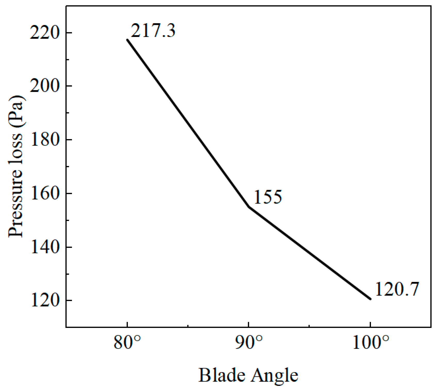
Figure 13 illustrates the pressure loss data along the axis for various blade clamping angles. It indicates a trend where pressure loss decreases as the angle of the mixing vanes increases. This phenomenon is primarily attributed to the effective area of the blade and its influence on flow resistance in the direction of flow. An increase in the blade angle corresponds to a sharpening of the blade relative to the flow direction. According to the model diagram, the projected or effective area of the blade in the flow direction diminishes as the blade angle increases. This reduction in effective areas lessens the impeding effect of the blades on fluid flow. Consequently, the blade clamp angle is a critical parameter in the design of a static mixer. By adjusting the blade angle, a balance can be achieved between mixing efficiency and energy consumption. Therefore, the optimal combination of mixing effectiveness and energy efficiency is attained by selecting the ideal blade angle, which should be determined based on the specific requirements of the application.
4.4. Fluid Velocity Analysis of the Static Mixer
Fluid is disrupted and redirected as it passes through the blades, resulting in a sharp change in the direction of the velocity field. The internal vanes in this section are designed with structural symmetry and feature flat surfaces, which enable the fluid flow in the mixer to exhibit significant symmetrical characteristics. The change in velocity direction is consistent on both sides of the blade due to this symmetry. Consequently, the velocity vector field on the symmetry plane serves as an appropriate basis for analyzing hydrodynamic behavior.
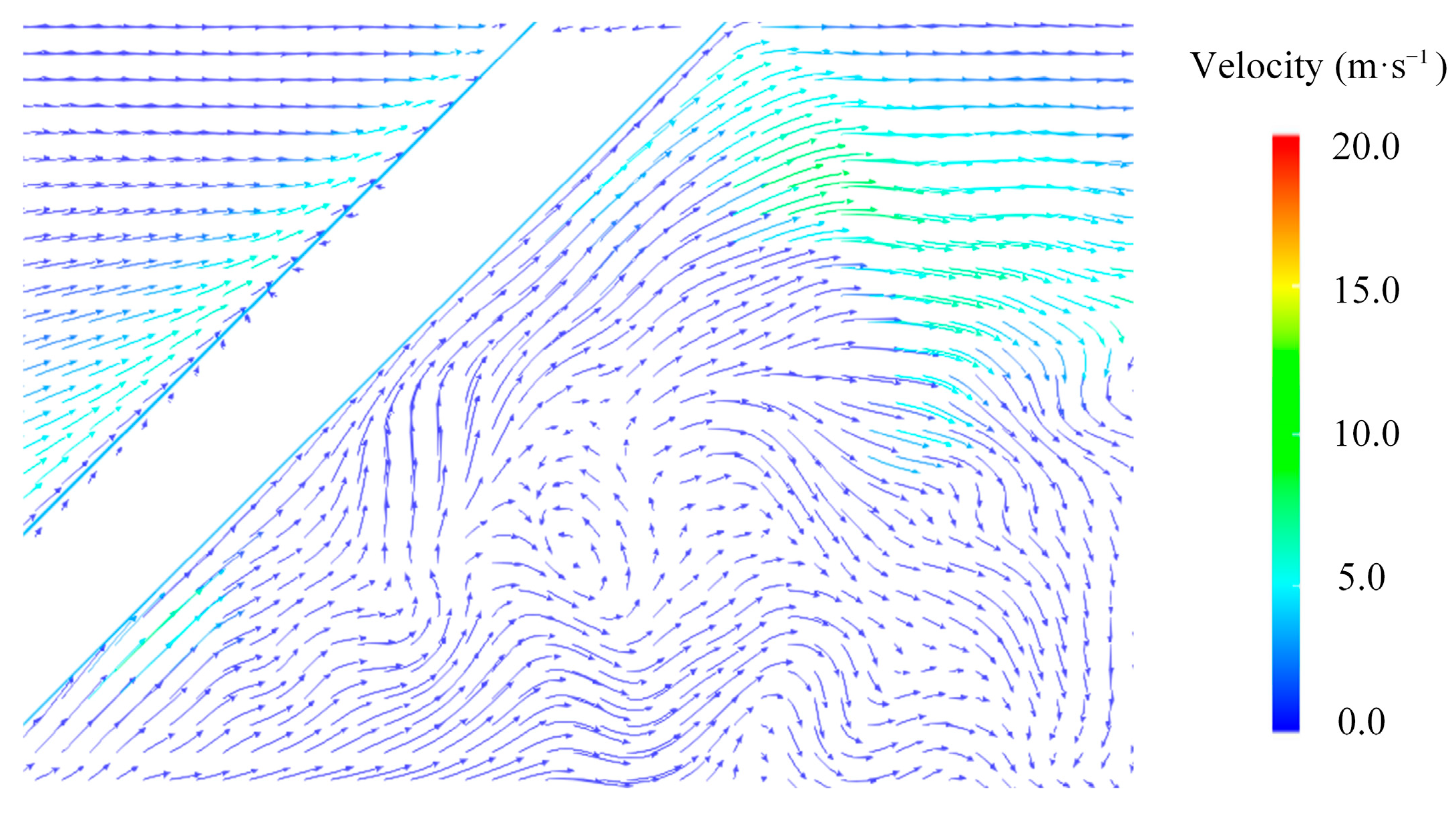
As the fluid flows through the vanes, the infusion action causes it to be split and diverted from both sides of the vanes. This process creates four segments of flow that are guided through the vanes by the flow-directing action. The fluid segments are mixed in pairs, resulting in two shear flows. The kinetic energy of the fluid is dissipated due to the blocking effect of the blades on the fluid flow, leading to a reduction in flow velocity and the formation of a low-velocity region behind the vanes. According to the principles of fluid dynamics, the low-pressure region and the abrupt change in flow direction are key factors in vortex formation. The results presented in
Figure 14 indicate that the vortices are primarily concentrated in the central region of the mixer, while a smaller number of vortices also appear near the wall surface. This observation suggests that convective mixing occurs between the central region and the wall region. The convective mixing contributes to the uniform distribution of the secondary phase (i.e., the fluid being mixed) and enhances mixing efficiency.
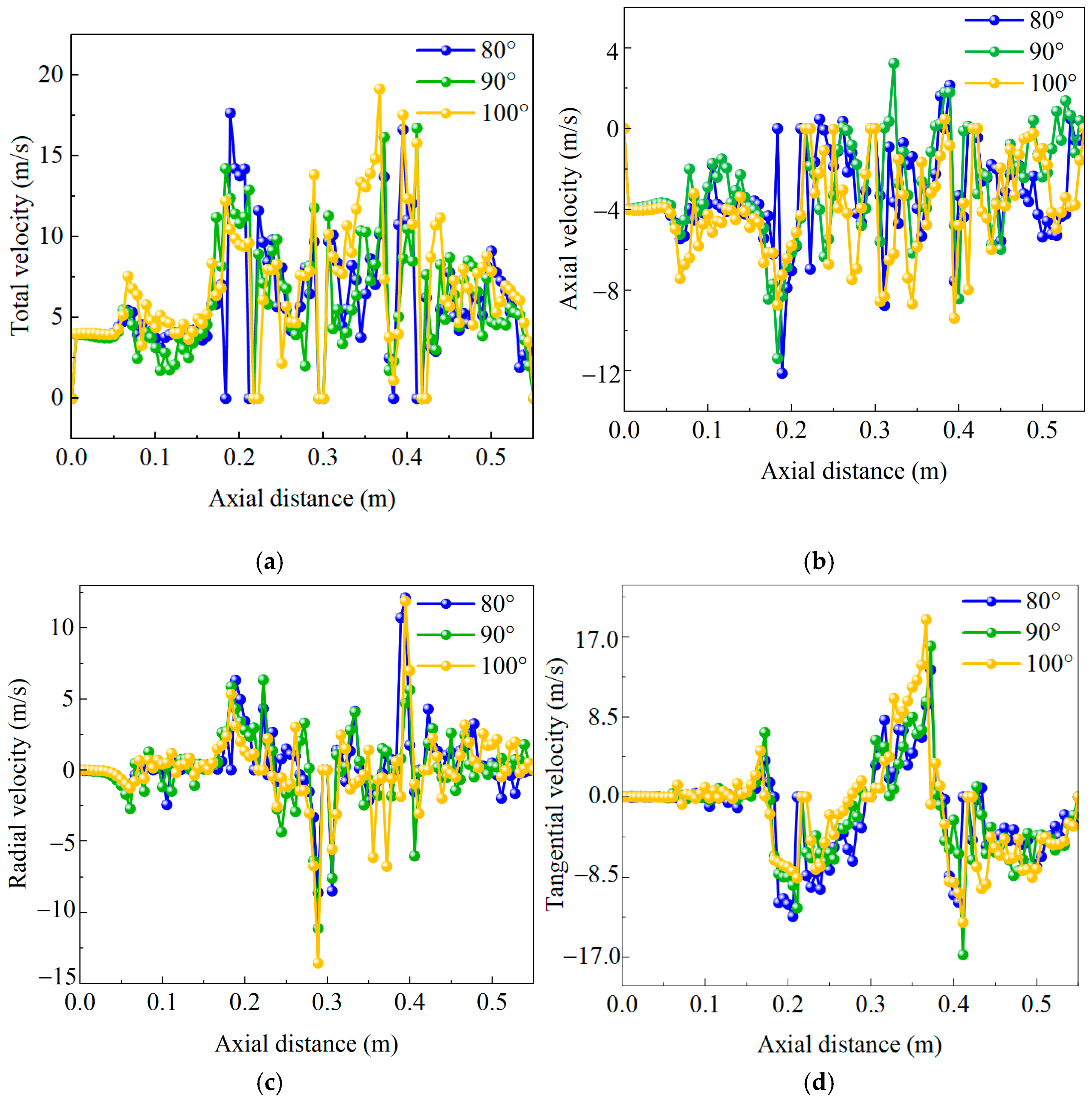
The overall trend and range of values of the velocity distribution curves are similar across the three different blade clamping conditions when comparing total, axial, radial, and tangential velocities. However, significant differences exist in the distribution of tangential and radial velocities compared to the distribution of axial velocities, as illustrated below. (1) The region near the blades exhibits higher velocities, indicating that the blades significantly influence the fluid flow. The angle of the blades also affects the fluid velocity, but this relationship is not linear. An increase in the blade angle does not consistently lead to an increase in the maximum velocity. (2) After passing through the first set of blades, the peak fluid velocity varies with different mixing blade angles of 80°, 90°, and 100°, ranging from low to high. The primary reason for this phenomenon is the change in fluid flow direction; as the direction changes, pressure decreases significantly, resulting in an increase in velocity. (3) The sudden increase in velocity is attributed to the convective collision of the fluid at radial inlet 2 with the axial kinetic energy of the flow field. These collisions cause a redistribution of energy, which enhances the total turbulent kinetic energy of the flow field. Although some of the energy may be dissipated through collisions, the overall velocity across the flow field increases. By analyzing the velocity distribution, valuable insights can be gained for the design of static mixers. For instance, by adjusting the angle and arrangement of the blades, the fluid’s velocity distribution can be optimized to achieve more efficient mixing.
The overall trend and range of values of the velocity distribution curves are similar across the three different blade clamping conditions when comparing total, axial, radial, and tangential velocities. However, significant differences exist in the distribution of tangential and radial velocities compared to the distribution of axial velocities, as illustrated below. (1) Both radial and tangential velocities experienced abrupt changes from zero after the fluid passed through the vanes. This indicates that the vanes significantly influence the direction and velocity of fluid flow. (2) By comparing the radial and tangential velocities at three different blade clamp angles, it can be observed that the amplitudes of these two velocities increase as the blade clamp angle increases. This suggests that the blade clamping angle is a crucial factor affecting flow characteristics and velocity distribution within the flow field. (3) Variations in the blade clamping angle have a substantial impact on the flow pattern and velocity distribution in the flow field. Such variations enhance the intensity of shear flow and return recoil, rendering the turbulence characteristics more complex and difficult to predict. (4) The function of the mixing vanes is to convert axial velocity in the flow field into tangential and radial velocities. The axial velocity decreases after passing through the blades, and its magnitude is lower than that of the tangential and radial velocities, as illustrated in
Figure 15. This velocity transition is critical for the mixing process, as it enhances mixing efficiency. These findings are significant for optimizing mixer design and operating conditions in engineering practice. By understanding how the blade pinch angle affects velocity distribution in the flow field, engineers can predict and adjust mixing effects and operating parameters to meet specific mixing requirements.
4.5. Uniformity Analysis of the Static Mixing
Mixing is the primary objective in the design of all mixers, and the effectiveness of mixing is a critical criterion for evaluating mixer performance. Among the various methodologies for assessing mixing efficiency, the coefficient of variation (COV) method has gained significant attention. This approach evaluates mixing performance based on the uniformity of component distribution within the mixing system. In this study, two fluid media are selected as mixing samples. Let the concentration of the dispersed phase be denoted as c1, where 0 < c1 < 1.c2 = 1 − c1. A radial cross-section of a static mixer is chosen as the sampling plane, which is further subdivided into n sampling regions. The sampling space is divided into the product of the surface area of each region and the mean velocity remains consistent across all regions. The area of each sampling region is determined according to this criterion. Therefore, the mean concentration of the dispersed phase on the radial cross-section can be expressed as follows:
where
c1.n represents the concentration of the dispersed phase in the
n-th sampling region. The standard deviation can be obtained:
The relative standard deviation (RSD) is described as follows:
The COV can be calculated by taking the ratio of the standard deviation to the mean and multiplying it by 100%. This ratio reveals the relative variability of the data and provide a scientific basis for evaluating mixing performance. The calculation formula is expressed as follows:
For a two-component system, the relationship between RSD, COV, and volumetric flow rate can be obtained:
Based on the above COV, when the COV value below 0.05 at the selected radial cross-section indicates that the mixer has achieved sufficient mixing effectiveness [
52,
53]. This standard is grounded in the stringent requirements for mixing quality in both experimental and industrial applications. In practical scenarios, a COV value of less than 0.1 is deemed acceptable for meeting mixing requirements. This suggests that the distribution of the mixed components is sufficiently uniform to satisfy the needs of most process operations. By establishing a threshold for the COV value, clear guidance can be provided for the design and operation of mixers.
In this section, a detailed analysis of the mixing effects under different actual operating conditions is conducted, with a particular focus on the impact of inlet velocity conditions and the variation in mixing blade angles on the mixing effect. By calculating the COV values for each longitudinal section, we can quantify the mixing uniformity under different conditions and compare the COV values of each condition to identify which parameters have a significant impact on the mixing process.
4.5.1. Effect of Inlet Velocity on the Mixing Uniformity
Figure 16 shows the mass fraction distribution of the dispersed phase (i.e., the fluid components being mixed) on the symmetry plane of a static mixer model with a blade angle of 90° under different inlet velocity conditions. These distributions are derived from the ratio of the mass of the dispersed phase to the total mass at the cross-section, which can provide an intuitive display of the mixing effect. As the flow rate increases, the mixing effect exhibits different characteristics in the figure. The angle at which the dispersed phase enters the mixer changes with variations in inlet velocity. Different inlet velocities affect the contact position of the dispersed phase with the blades, thereby influencing the mixing effect. In
Figure 16a,b, at lower flow rates, the mixing is more uniform, as the fluid has sufficient time to mix under the action of the blades. However, in
Figure 16c,d, at higher flow rates, the mixing is insufficient, leading to an uneven mass fraction distribution. In
Figure 16d, the mass fraction distribution is different from that at other flow rates. This is because, at very high flow rates, the inertial effects of the fluid become more pronounced, resulting in changes in the mixing effect.
At all flow rates, the distribution of mass fraction shows a higher mixing effect near the blades, which is due to the guiding and shearing action of the blades on the fluid. When the secondary phase comes into contact with the blades at the center of the pipe, it is split into two streams by the blades, which then flow around the blades and rejoin behind them. During this process, the fluid velocity changes and flows along the axial direction, facilitating the diffusion of the secondary phase in the radial direction of the cross-section, thereby enhancing the mixing effect. Furthermore, if the secondary phase contacts the blades on the upper or lower side, it will move along the blade surface, creating a rotating flow field. In this case, some fluid may merge, but the overall flow field becomes asymmetrical, and the mixing effect is lower than when the secondary phase contacts the blades at the center.
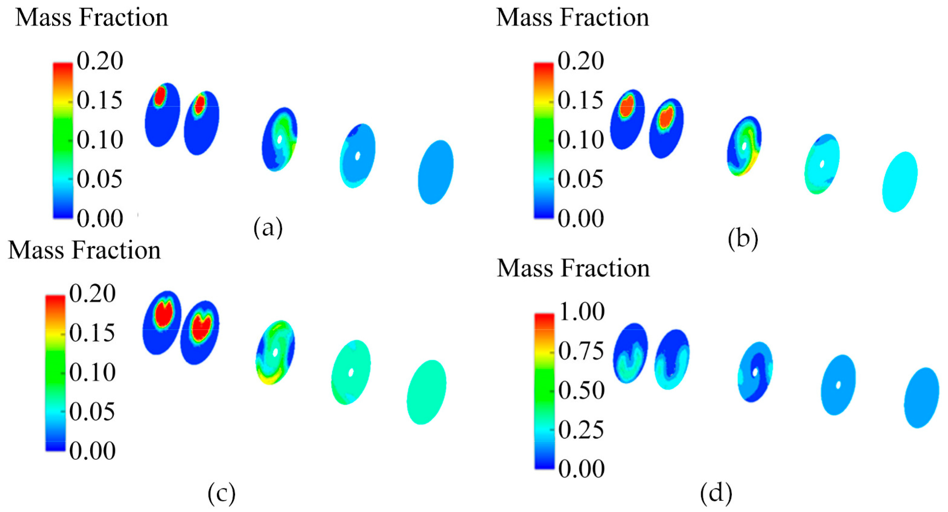
Figure 17 provides a detailed depiction of the mixing effect distribution of a static mixer in the radial cross-section, reflecting the impact of different inlet velocities on mixing uniformity. In
Figure 17a–c, it can be observed that the mass fraction of the dispersed phase gradually decreases from left to right, indicating that as the fluid flows through the mixer, the dispersed phase gradually mixes with the continuous phase, leading to a more uniform mass fraction. The shear effect of the blades plays a crucial role in the uniform distribution of the mass fraction. Under the action of the blades, the fluid is effectively divided and recombined, resulting in a symmetrical mass fraction distribution. It is a result of the optimization of the blades in the mixer design. In
Figure 17d, the mass fraction at the inlet is low, which may be due to the inertial effects of the fluid at high flow rates, leading to less pronounced mixing effects during the initial mixing stage compared to lower flow rates. However, as the fluid continues to flow through the mixer, the mixing effect improves. By the fourth cross-section, the mixing effect has become relatively uniform, indicating that at this position, the fluid medium has undergone sufficient shear and recombination, and achieved a good mixing state.
In general, the greater the inlet velocity, the greater the kinetic energy of the fluid. When encountering the blades, this kinetic energy is converted into the energy of shear flow, enhancing the mixing effect. This energy conversion is significant at high flow rates, helping to disperse the fluid medium. The flow characteristics of the fluid at high velocities are more chaotic, and this chaos is beneficial for improving mixing efficiency. Chaotic flow can promote the random mixing of fluids, leading to a more uniform spatial distribution of fluid components. These analytical results are of great importance for the design of mixers and the optimization of operating conditions in engineering practice. By understanding the impact of different inlet velocities on mixing effects, engineers can predict mixing outcomes and adjust operational parameters to meet specific mixing requirements.
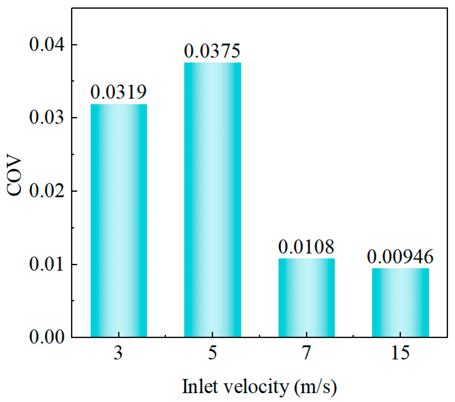
During the study of the static mixer model, the COV at the outlet under different inlet velocities is calculated, and the results are organized in
Figure 18. By comparing the outlet COV values at different inlet velocities, it is found that the COV value is the smallest when the inlet velocity is 15 m/s. This result is consistent with theoretical analysis, which indicates that at higher flow rates, the mixing effect is better due to the increased kinetic energy of the fluid, leading to more intense shear flow and more effective mixing. The COV values at other inlet velocities correspond to the variation in mass fraction across the cross-section. This suggests that the COV value can reflect the uniformity of fluid mixing within the mixer. The data show that as the inlet velocity increases, the COV value tends to decrease. When assessing mixing performance, a COV value of less than 0.1 is considered to indicate a uniform state. This standard provides us with a quantitative indicator to evaluate the mixing effect. Therefore, when the inlet velocity is 3 m/s, the COV value is far less than 0.1. This indicates that the mixer at this velocity can achieve a good mixing effect while avoiding excessive energy consumption. Thus, the 3 m/s is a relatively ideal inlet velocity.
4.5.2. Effect of Blade Angle on the Mixing Uniformity
This section analyzes the mixing effects of three different static mixer models with blade angles of 80°, 90°, and 100°. To evaluate the mixing performance of these models, we focused on the mass fraction distribution of the secondary phase (i.e., the fluid component being mixed) at the moment of 0.2 s, when the inlet speed of inlet 1 is set to 7 m/s.
Figure 19 illustrates the impact of blade angle variation on the circumferential and radial diffusion of the dispersed phase (i.e., the components of the mixed fluid) in a static mixer. The following patterns can be observed: (1) A decrease in blade angle promotes circumferential flow while weakening radial and axial flows. This change in flow pattern aids in the uniform distribution of the dispersed phase across the mixer cross-section, as circumferential flow can push the dispersed phase to diffuse outward, enhancing the mixing effect. (2) When the blade angle increases, circumferential flow weakens while radial and axial flows are strengthened. This flow pattern helps maintain a uniform distribution of the dispersed phase across the cross-section, preventing the occurrence of dispersed phase deficiency in the center area. (3) In
Figure 19a,b,e,f, the mass fraction distribution of the dispersed phase at the wall in the third cross-section shows significant non-uniformity, and at the fourth cross-section, the mixing uniformity at the wall has still not improved. (4)
Figure 19c,d show that at the third cross-section, a balance between circumferential and radial flows is achieved, which contributes to a dynamic balance of the mixing state. By the fourth cross-section, the mixing uniformity has significantly improved, and compared to the other two models, the model with a blade angle of 90° achieves a uniform mixing state earlier. By comparing the models with three different blade angles, it can be concluded that the model with a blade angle of 90° performs best in terms of mixing effect and efficiency. This indicates that the choice of blade angle is crucial for achieving efficient mixing in the design of static mixers.
The COV values at the outlet of static mixer models with three different blade angles (80°, 90°, and 100°) were calculated under an inlet velocity of 7 m/s, and the results are summarized in
Figure 20. The analysis reveals a significant impact of the blade angle on the mixing effect. The model with a blade angle of 90° exhibited the lowest COV value, which is consistent with the observation of the cross-sectional mass fraction distribution shown in the previous figure, indicating that the mixing effect is most uniform at this angle. As the blade angle increases, the COV value reaches a minimum near 90° and then rises with further increases in the angle. This indicates that a blade angle of 90° has an advantage in mixing performance, facilitating more effective fluid mixing. Considering both the mixing effect and energy efficiency, the model with a blade angle of 90° demonstrates the best mixing effect and efficiency. This finding provides important guidance for the design of static mixers, enabling engineers to select appropriate blade angles to achieve efficient mixing.
5. Conclusions
Investigating the mixing transfer mechanisms and optimization design of two-phase flow in static mixers is of great significance for improving the mixing efficiency and stability of flow control devices in fields such as aviation, nuclear power, and new energy. This study presents a novel numerical framework that integrates the lattice Boltzmann method (LBM) with large eddy simulation (LES) and octree lattice block refinement to overcome limitations of conventional CFD approaches in capturing complex, nonlinear two-phase flow dynamics in static mixers. This paper proposes a modeling and solving method for the two-phase flow mixing transfer dynamics of static mixers based on the LBM and LES. It explores the dynamic characteristics of two-phase flow mixing and optimization design strategies under complex component structures. The relevant research work has been completed, and the main conclusions are as follows:
- (1)
Based on the LBM and MRT-WALE vortex viscosity model, combined with the octree lattice block refinement method, a mixing transport dynamic model of two-phase flow in a static mixer has been established. This model is used to study the interaction mechanism between the fluid and the wall during the mixing process and analyzes the dynamic changes in parameters such as turbulent kinetic energy, velocity, and pressure drop under different flow rates and configurations of mixing elements.
- (2)
Blade components significantly influence the dynamic characteristics of the mixing flow field. The blades serve as the main driving force for the increase in turbulent kinetic energy. Low-speed and low-pressure regions tend to form downstream of the blades, causing abrupt changes in flow direction. In high-turbulence regions, vortices are more likely to develop, enhancing the overall mixing effect. When the blade angle increases from 80° to 100°, the pressure drop is reduced by approximately 44%, indicating that larger blade angles effectively lower flow resistance. However, this also implies a potential trade-off, as reduced shear may diminish the mixing strength.
- (3)
The blade angle is a critical parameter affecting pressure loss in static mixer systems. When fluid encounters the blades, the resulting obstruction, energy dissipation, and sharp changes in flow direction cause a stepped decrease in static pressure. As inlet velocity increases from 3 m/s to 15 m/s, the pressure drop rises by more than 23 times, indicating a sharp increase in resistance with flow rate. While a smaller blade angle enhances turbulent mixing, it also causes significantly higher pressure loss—approximately 80% more than that at a larger blade angle—thereby increasing system energy consumption. Optimal design must therefore balance flow resistance with mixing effectiveness.
- (4)
Inlet velocity and blade angle jointly impact the mixing efficiency. An increase in inlet velocity significantly improves mixing performance: the outlet COV value drops by around 70.3% when the inlet velocity rises from 3 m/s to 15 m/s, suggesting much better uniformity in phase distribution. However, this improvement comes at the cost of sharply increased energy consumption due to higher pressure losses. As for blade angles, the COV first decreases and then increases with the angle, reaching a minimum at 90°, which reflects the most efficient mixing condition. Therefore, a configuration with moderate inlet velocity (e.g., 3 m/s) and a blade angle of 90° achieves an optimal balance between mixing performance and energy efficiency.
Although the LBM–LES approach effectively captures the multi-scale turbulence characteristics and complex geometries involved in static mixer flows, it entails considerable computational cost, especially when applying high spatial resolutions or conducting parameter sweeps for optimization. Additionally, assumptions in subgrid turbulence modeling may limit accuracy in near-wall regions or in flows with strong anisotropy. Future work will focus on experimental validation of the simulation results to improve model credibility and guide engineering applications. Moreover, incorporating multi-objective optimization methods that balance mixing efficiency, pressure drop, and energy consumption will be explored to support practical design decisions.


 and
and 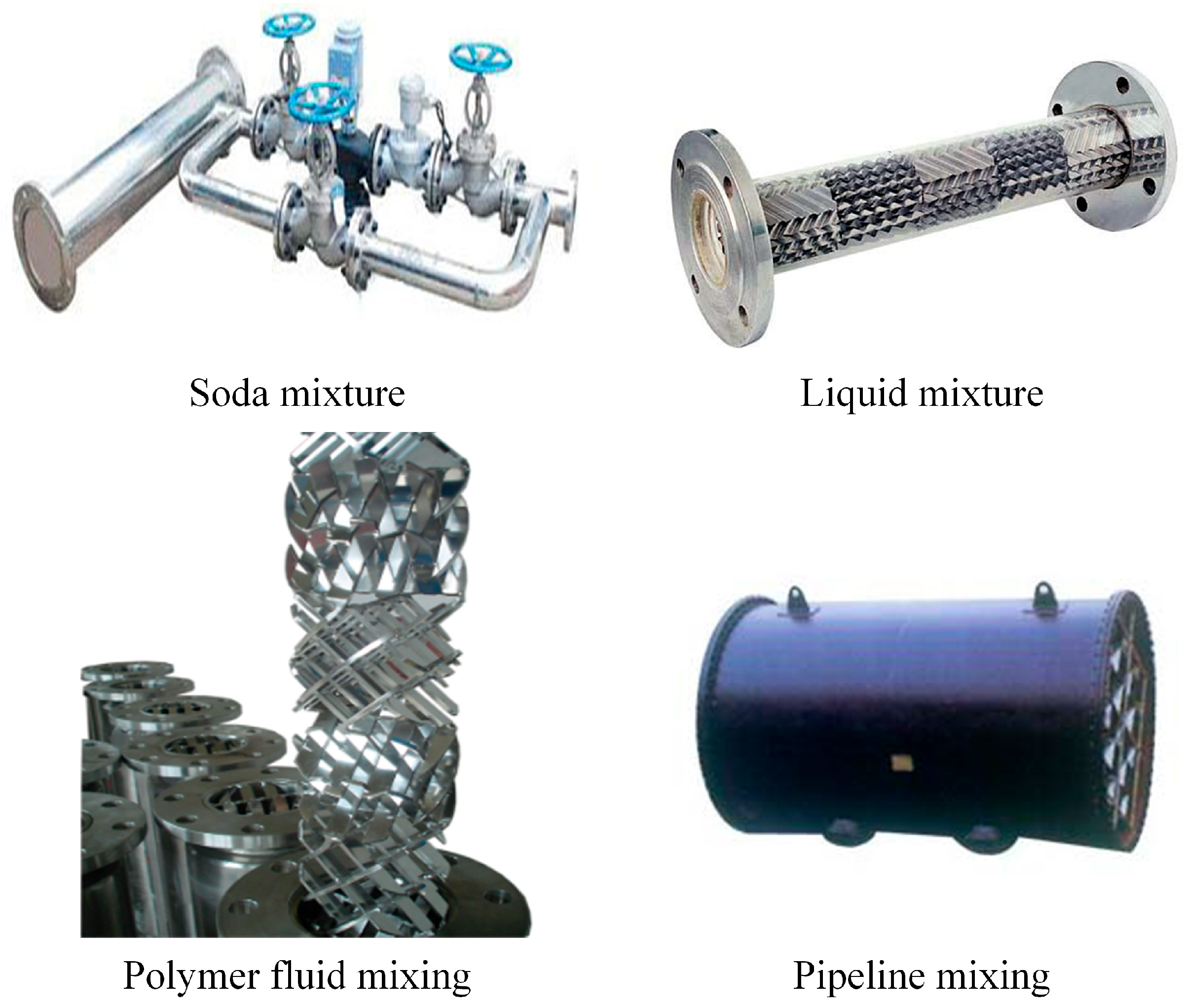


