Abstract
With the increase in exploration in recent years, buried hill condensate gas reservoirs have gradually become an important field for increasing reserves and production of offshore oil and gas in China, and efficient development of condensate gas reservoirs has also become a hot issue in hydrocarbon development. Due to the complex phase-change law and retrograde condensation phenomenon of deep condensate gas reservoirs, the reservoir properties and production dynamics data obtained by conventional pressure-recovery-test methods were greatly limited, and the dynamic data and evaluation parameters of the single well control area cannot be accurately determined. In this paper, using the production analysis method to analyze the production dynamics data of a single well, combined with static geological data and well-test analysis data, the reservoir parameters of a single well were evaluated. Specifically, the Blasingame method was applied to realize the production-decline law of production wells, and new dimensionless flow, pressure parameters, and pseudo-time functions were introduced. Using the unstable well test theory and the traditional production decline analysis technology, the IHS Harmony software is used to fit the production dynamic data with the theoretical chart. The evaluation parameters such as reservoir permeability, skin factor, well control radius, and well control reserves were calculated, providing strong support for the production decision-making of the petroleum industry and also providing a strong decision-making basis for the dynamic adjustment of oil–gas-well manufacture.
1. Introduction
Accurate determination of reservoir parameters and yield dynamic evaluation parameters can provide help for the efficient development of oil–gas wells. Certain reservoir parameters can be obtained through pressure-recovery tests, and yield dynamic evaluation parameters can be obtained based on modern production-decline analysis [1]. Because the buried hill condensate gas reservoir in the central Bohai Sea is a condensate gas reservoir with near-dew-point pressure and high condensate oil content, it has the characteristics of low porosity and low permeability, strong heterogeneity, complex spatial distribution of oil–gas reservoirs, uneven growing of cracks, and high water saturation [2], which lead to the pressure-recovery well test in most cases. It is not easy to obtain reservoir properties and yield dynamics data [3]. As a modern yield-decline analysis method [4], the Blasingame method adopts the pseudo-pressure normalization yield (q/P) and matter equilibrium pseudo-time (tc) functions and establishes a typical curve chart of productivity decline based on closed depleted gas reservoirs and fully considers the characteristics of gas PVT physical properties changing with formation pressure [5]. This method has various interpretation models, such as vertical wells, fracturing wells, and horizontal wells, which can analyze the dynamic data of gas wells in the whole production stage. The interpretation results are more objective than results of well-test analysis in reflecting the actual situation of the formation. The complex method has various interpretation models such as vertical wells, fracturing wells, and horizontal wells, which can analyze the dynamic data of gas wells in the whole production stage. The complex variable pressure and variable production problem is transformed into a unified fixed bottom hole pressure, which reduces the difficulty of the work. Through the fitting analysis of production data and theoretical charts, the evaluation parameters such as reservoir permeability, skin factor, well control radius, and well control reserves can be calculated [6].
As a modern production-decline analysis method, Blasingame has a wide and far-reaching application in production dynamics analysis. Fraim [7,8] defined the normalized time, combined the pseudo-steady-state gas well productivity equation ignoring non-Darcy flow with the material balance equation, obtained the normalized time and gas well production function with an exponential decline relationship, and established the gas well production-decline chart-fitting method. Spivey, Gatens, and Lee [9] established a new typical curve chart using dimensionless yield and dimensionless cumulative yield under logarithmic conditions. This method was easier to fit and compare than the yield curve. In addition, the cumulative yield curve at the later stage of flow could obtain more data. Pratikno, Rusing, and Blasingame et al. [10] established a production dynamics model of finite conductivity vertical fracture wells under circular boundary conditions and drew a typical decline curve suitable for interpretation and analysis of production data in low permeability reservoirs.
After decades of development, the production-dynamics analysis method has gradually developed from the traditional empirical method into various types of production dynamics analysis models. Gradually breaking through the limitations of each production-dynamics analysis method in the use process [11], the analysis results ranged from basic single-well-controlled reserve prediction to accurate acquisition of various reservoir evaluation parameters [12]. Based on the introduction of the principle and the Blasingame production-decline analysis method, this paper analyzes the production dynamics of a deep condensate gas reservoir in the sea and obtains a series of evaluation parameters, which provide a basis for the dynamic analysis of condensate gas reservoir production.
The software version used in this article is IHS Harony 2016 v3, FAST Harmony (Fekete Associates Inc., Calgary, AB, Canada)
2. Principle of the Blasingame Method
2.1. Unsteady Flow and Boundary Flow
The flow of gas in a gas reservoir with a boundary can be divided into an early unstable-flow stage and a later boundary-flow stage [13]. At the beginning of the floating, the pressure change has not yet spread to the border of the gas accumulations, and the border will not affect the floating. In the later phase of the floating, the pressure drop propagates to the border of the gas accumulations, and the border has an influence on the floating. Quasi-steady flow is a case of boundary flow [3,14].
The relationship between dimensionless yield and dimensionless time is demonstrated in Figure 1. The pressure curve shows the characteristics of early linear flow, middle radial flow, and late boundary control flow (quasi-steady state) [15].
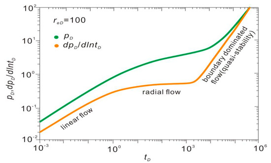
Figure 1.
Unstable flow pressure and pressure derivative curve of fixed production.
2.2. Material Balance Equivalent Time and Pseudo−Time
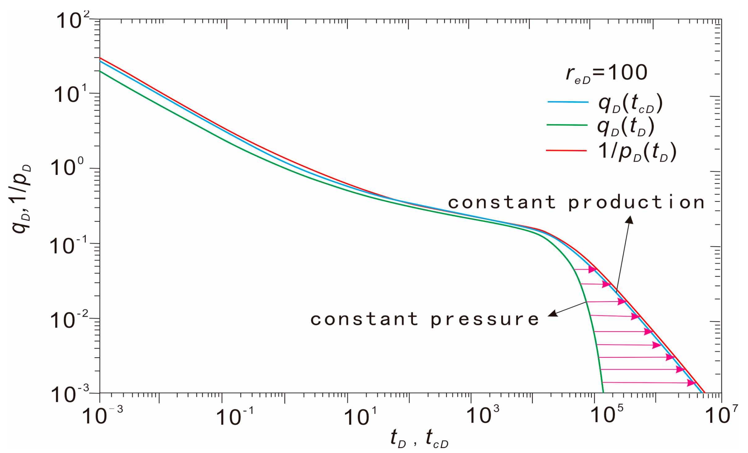
As shown in Figure 2, the output solution qD of constant pressure production and the reciprocal 1/pD of the pressure solution of constant production are plotted on a graph. The two curves basically coincide in the unstable flow stage and are separated in the boundary control flow stage [16]. In order to make the two curves coincide in the boundary control flow stage, Blasingame applied the dimensionless matter equilibrium time tcD to replace the dimensionless time tD. The results show that the two curves coincide completely. Therefore, the introduction of tcD makes the variable production solution equivalent to the fixed production solution so that the Blasingame method can be applied to the two cases of variable production and variable bottom hole flow pressure [17,18].
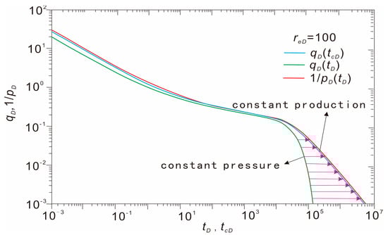
Figure 2.
Constant pressure reciprocal, constant pressure yield, and constant pressure material balance time−yield comparison curve.
In order to consider the change in gas PVT properties with pressure in the depletion development of gas reservoirs, the normalized pseudo−pressure and pseudo−time are introduced to analyze the well test. The pseudo−pressure simplifies the well−test interpretation process by linearizing the nonlinear gas flow problem [19].
The normalized pseudo−pressure is defined as The quasi-time of material balance is defined as In the above formula,
qD—the output solution of constant pressure production;
tcD—dimensionless material equilibrium time;
tD—dimensionless time;
Pp—regularized pseudo-pressure;
pD—dimensionless production;
μ—fluid viscosity;
Z—gas compressibility factor.
2.3. Condensate Gas Reservoir Retrograde Condensation Phenomenon
There are complex phase changes in the development of condensate reservoirs. During the development process, when the formation pressure decreases below the dew-point pressure, the heavy hydrocarbon components in the gas will undergo retrograde condensation, causing the change in fluid-phase state and the precipitation of condensate oil from the gas, which has a great influence on the seepage characteristics of the condensate oil and gas system. On the one hand, the decrease in the content of condensate oil in the gas phase leads to the change in permeability characteristics; on the other hand, the existence and distribution of condensate oil will affect the condensate gas flow to the wellbore, and this effect changes with time.
In the process of condensate gas reservoir development, retrograde condensation will occur in the condensate oil and gas system. With the development of depletion in condensate gas reservoirs, when the formation pressure drops to a certain pressure range (maximum condensate pressure) below the initial condensate pressure (upper dew-point pressure), part of the condensate oil will precipitate in the reservoir and remain on the pore surface of the reservoir rock, resulting in loss. The phase state and composition of the condensate oil and gas system can change with pressure and temperature at any time and anywhere. Moreover, the interface characteristics such as adsorption, capillary force, capillary condensation, and rock wettability in porous media and the existence of bound water will affect the phase state of oil and gas and condensate gas production.
Changes in thermodynamic conditions (pressure, temperature, and composition) that cause changes in the composition and phase state of condensate gas wells will also directly affect the surface recovery of condensate oil and other hydrocarbons.
2.4. Well-Test Interpretation Model of the Condensate Gas Pool
A well-test explanation is the process of analyzing the test data in detail after the well test of an oil–gas well is completed. Well testing usually involves measuring the flow rate, pressure, fluid properties, and other parameters of the well to evaluate the performance of the well and the characteristics of the reservoir [20]. The purpose of well-test interpretation is to determine the productivity of the well, identify potential production problems, evaluate the dynamic characteristics of the oil pool, and provide evidence for subsequent development decisions [21].
The data provided by well-test interpretation are helpful in establishing a more accurate reservoir model [22]. For modern production-decline analysis, the establishment of an accurate well-test interpretation model has an important role in promoting the selection of the corresponding Blasingame interpretation model and the establishment of the composite chart so that more accurate oil and gas well evaluation parameters can be obtained. This is very important for production prediction and development planning in production dynamics analysis [23].
However, the establishment of a well-test analysis and well-test interpretation model of condensate gas wells is a difficult research topic: for condensate gas reservoirs, it is essentially a multiphase flow well test in well-test analysis, and the formation pressure data have a considerable impact on the seepage of the condensate gas reservoir [24]. When the formation pressure is higher than the dew-point pressure, the seepage characteristics of the condensate gas reservoir are not much different to those of the dry gas reservoir. When the formation pressure is lower than the dew-point pressure, the condensate oil will be precipitated from the formation, resulting in the coexistence of oil and gas [25]. The condensate gas reservoir has special properties that conventional multiphase flow well testing does not have: reservoir seepage is affected by various factors and the fluid properties are multi-component gases with complex phase changes [26]. The reservoir effect of the well is more obvious [27]. The establishment of a well-test interpretation model also becomes more difficult due to these factors.
Due to the complexity of the condensate gas reservoir [28], the model used is different from the general well-test interpretation model, and the following models are commonly used [29]:
- (1)
- Variable well storage model: The variable well storage model takes into account the change in wellbore storage coefficient with time, which is suitable for the complex wellbore conditions or the change in fluid-phase state.
- (2)
- Dual-porosity medium model: For condensate gas reservoirs with fractures, this model can describe the flow of fluids in the matrix and fractures and the fluid exchange between the two.
- (3)
- Composite model: This model is used to describe multi-layer reservoirs with different fluid flow characteristics. Each layer can have different porosity, permeability, and saturation.
- (4)
- Vertical and horizontal fracture model: This model is suitable for reservoirs with vertical or horizontal fractures. It can also be used to describe the effect of fractures on fluid flow.
- (5)
- Component model: The fluid in the condensate gas reservoir is multi-component. The component model can simulate the migration and phase change in components, especially when the pressure and temperature change.
- (6)
- Pseudo-pressure model: Because the flow characteristics of condensate gas are different from those of conventional gas, the pseudo-pressure model adapts to the characteristics of condensate gas reservoirs by modifying the definition of pressure.
2.5. Blasingame Composite Plate
The Blasingame modern production analysis chart introduces the pseudo-regularized pressure and material balance time function to consider the production situation of variable bottom hole flow pressure [30]. After optimization and improvement, the established chart can be applied to the production fitting of complex well types such as horizontal wells, fractured wells, and vertical wells [31]; it is also suitable for composite, homogeneous, double permeability, and triple porosity medium models [32]. In the interpretation model, it also includes a vertical-well fracture model, a vertical-well radial model, a horizontal-well model, a water-flooding model, and an inter-well interference model [33], and the scope of interpretation is more extensive.
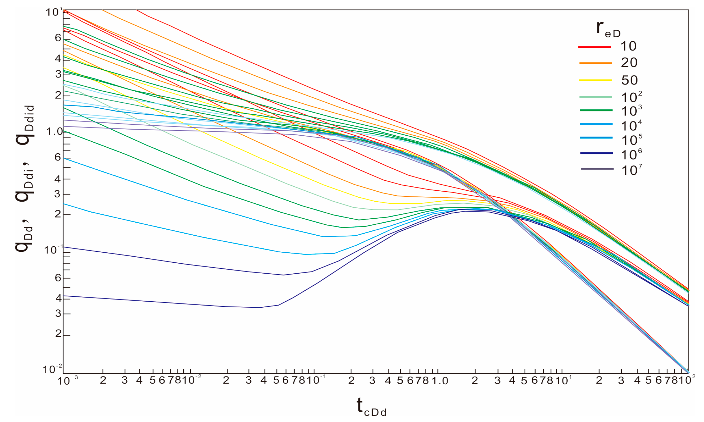
When drawing the Blasingame modern yield analysis chart, the dimensionless time is used as the abscissa, and the dimensionless yield, dimensionless yield integral, and dimensionless yield integral derivative are used as the ordinate to draw the curve [34]. These three curves constitute the Blasingame composite chart curve (Figure 3). After introducing the material balance quasi-time function, the three curves of the typical production chart are normalized to a harmonic decline curve in the boundary control flow stage [35]. Then, the production data of the actual well are fitted with the chart to calculate the evaluation parameters such as permeability K, skin coefficients, well control radius re, and original geological reserves G, so as to realize the evaluation of formation physical properties and reserves in the single well control area [36].
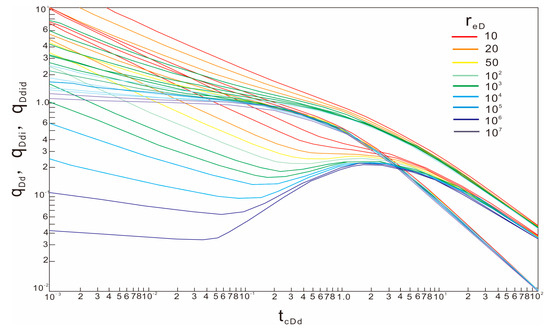
Figure 3.
Blasingame composite plate.
3. Blasingame Method Fitting Analysis
During the course of modern production−decline analysis, the dimensionless time is used as the abscissa, and the dimensionless production, dimensionless production integral, and dimensionless production integral derivative are used as the ordinate to draw the curve. These three curves constitute the Blasingame composite chart curve [37].
Using the actual well production data and the Blasingame composite chart curve to fit, in the process of production data fitting, the actual gas well production data and the producing bottom hole pressure date are used to calculate the fitting time, predict the yield under the unit pseudo−pressure, and draw the relationship curve between the fitting time and the yield in the double logarithmic coordinates [38]. Finally, the measured data curve are fitted with the chart curve. In order to obtain a better fitting effect, the above steps are cycled, and then any one of the fitting points is selected in the process. The actual fitting point and the corresponding theoretical fitting point are recorded, and the permeability according to the yield fitting point is calculated [39,40]; the calculated permeability and dimensionless well control radius [41], and the effective well diameter of the production well are then calculated according to the time fitting point. The skin factor is calculated according to the effective well diameter and wellbore radius. The well control radius and well control reserves are calculated according to the obtained parameters [42]. Finally, according to the obtained evaluation parameters, the evaluation of formation physical properties and reserves in the single well control area is realized [43,44].
In order to standardize the application of the Blasingame production−decline analysis method in actual gas−reservoir analysis, Sun Hedong et al. have given detailed analysis steps for the Blasingame curve-fitting analysis method. The specific steps are as follows:
- (1)
- According to the geological parameters, such as the range of the well control area, an original geological reserve G is assumed.
- (2)
- According to the production of different mining times and the material balance equation, the formation pressure pp of different mining times is calculated.
- (3)
- The material balance time under each production point is calculated:
- (4)
- Using to the production data of gas wells, combined with the proposed production pressure difference, the normalized production of each production point is calculated as follows:
- (5)
- Based on the material balance time and the normalized yield, the integral calculation of the normalized yield is realized:
- (6)
- The derivative of the normalized cumulative yield integral is obtained by the derivative of the normalized yield integral to the material balance time, and the judgment of the change speed of the normalized yield integral is realized:
- (7)
- A (ppi−pp)/q—tca rectangular coordinate curve is drawn and the geological reserves G are calculated according to the slope of the regression line:
This is compared with the original reserves of step (1). If the error is large, steps 2–6 are repeated with the new original geological reserves until convergence, meeting the allowable error of G, and ending the iterative calculation.
- (8)
- The double logarithmic curves of q/∆pp, (q/∆pp)i, and (q/∆pp)id—tca are drawn in the rectangular coordinate system on the semi-transparent paper, and the drawn curves are fitted with the Blasingame typical chart curve (Figure 3) to obtain better curve-fitting results. According to the fitting results, the dimensionless well control radius reD is recorded.
- (9)
- A better-fitting point is chosen, and the actual fitting point (tca, q/∆pp)m and the corresponding theoretical fitting point (tcaDd, qDd)m are recorded. The evaluation parameters such as reservoir permeability, skin factor, well control radius, and well control reserves can be calculated according to the actual fitting point, theoretical fitting point, and dimensionless well control radius.In the above formulae,tca—material balance pseudo-time;Ct—composite compressibility;P—pressure (MPa);q—daily production (104 m3/d);K—permeability (mD);s—skin coefficient;re—well control radius (m);G—original geological reserves (108 m3);Pi—original formation pressure (MPa);Pwf—bottom hole flowing pressure (MPa);B—volumetric coefficient;h—strata thickness (m);Φ—formation porosity;reD—dimensionless well control radius;rw—wellbore radius (m);rwa—effective wellbore radius (m);i—integral;D—differential coefficient.
4. Blasingame Method Instance Application
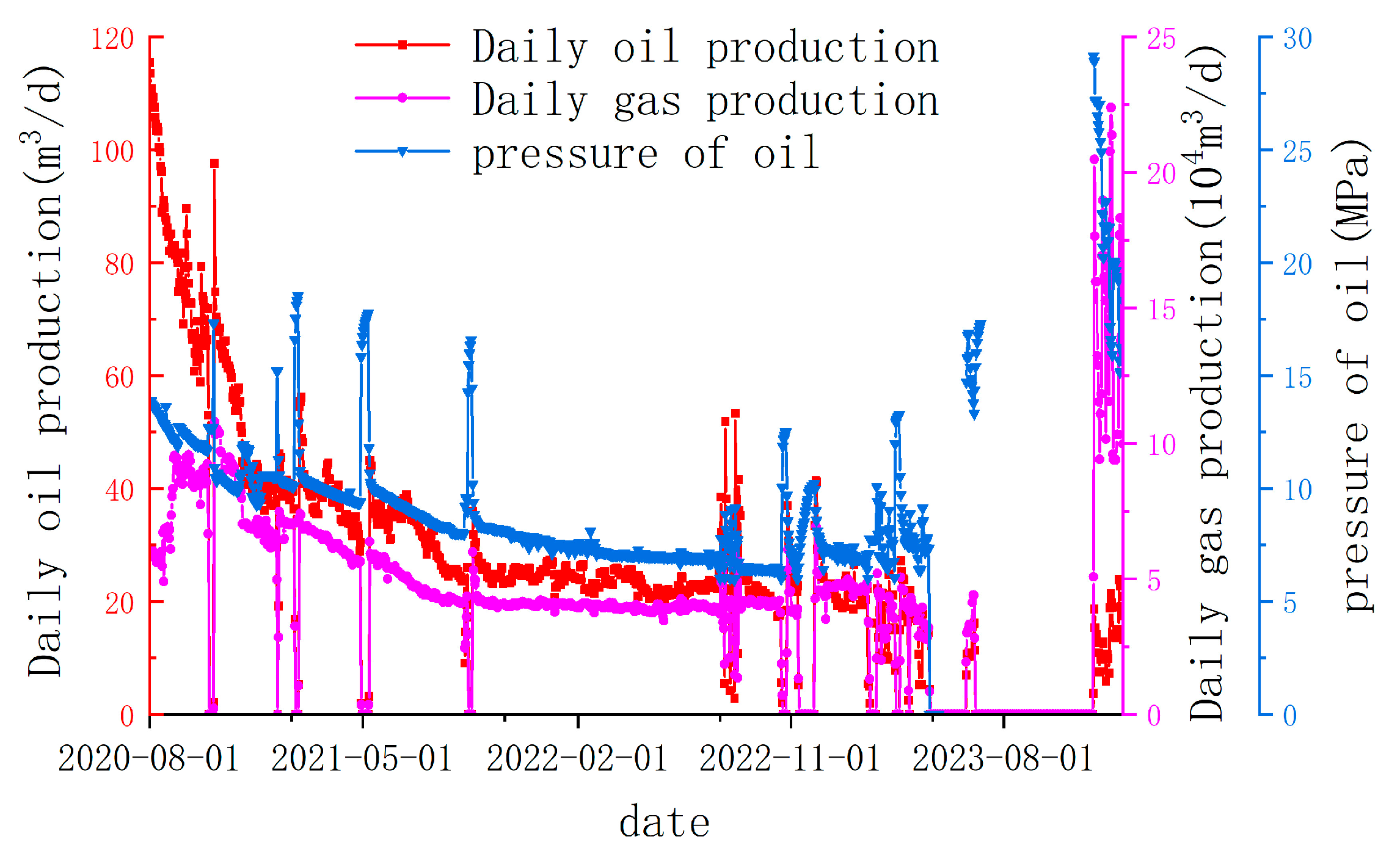
The research region is situated in the center of the Bohai Sea. It is mainly a condensate gas reservoir with near−dew−point pressure and high condensate oil. Well A is a horizontal well that goes into operation in the pilot area of the gas−condensate reservoir. On 26 July 2020, Well A was opened for trial production. The initial nozzle was 9.44 mm and the daily oil production was 131 m3. After that, the liquid production gradually decreased, and the oil pressure gradually decreased. As of January 2024, the cumulative oil production of the well was 3.18 × 10⁴ m3, and the cumulative gas production was 0.5365 × 10⁸ m3. he production data change curve of Well A in the whole production process is shown in Figure 4.
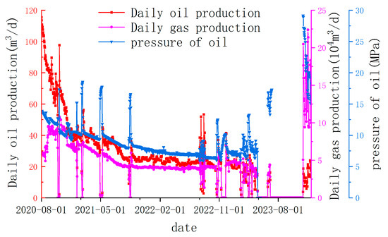
Figure 4.
Dynamic change diagram of production data in the production process of Well A.
From the dynamic variation diagram of operating data of production from Well A, from August 2020 to August 2021, the daily oil production decreased sharply, and the daily gas production and oil pressure decreased steadily. From August 2021 to May 2023, oil pressure, daily gas production, and daily oil production basically stabilized.
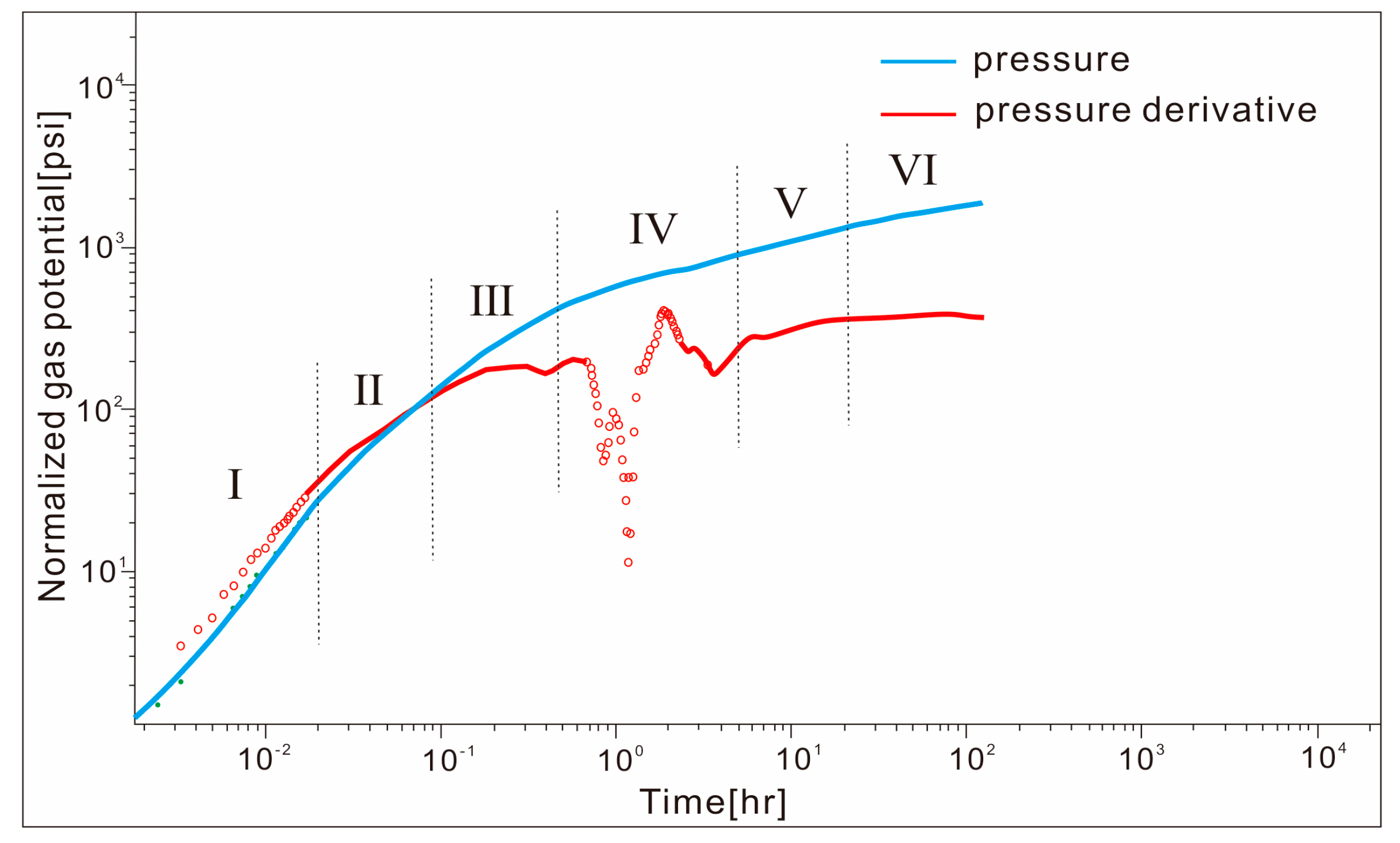
In order to understand the well control area and reservoir physical properties of the well, the flow pressure + pressure recovery + static pressure test operation was carried out on the well in September 2020, and reliable pressure-recovery data were obtained. In order to select a more accurate well-test interpretation model, the pressure-recovery double logarithmic curve was divided into stages, and the characteristics of each stage were analyzed in detail. The division results are shown in Figure 5.
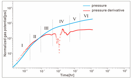
Figure 5.
A well pressure−recovery double logarithmic curve stage division diagram.
Stage I: Wellbore storage stage. This stage includes two stages: the pure wellbore stage and the transition stage. The pressure and pressure derivative curves are unit slope straight lines;
Stage II: With the continuous production of horizontal wells, the pressure continues to spread outward, the seepage resistance increases, and the differential of the pressure curve continues to warp;
Stage III: Radial flow reflection stage, horizontal straight line characteristics of the differential of the pressure curve;
Stage IV: The typical flow characteristics of the dual−porosity medium reservoir and the channeling section of the matrix to the fracture are obvious; the deeper the concave of the derivative curve, the smaller the elastic storage ratio, and the larger the proportion of the matrix storage fluid;
Stage V: The curve has a rising trend, showing linear flow characteristics, indicating that there are fractures in the formation;
Stage VI: The later quasi-radial flow segment is not fully apparent.
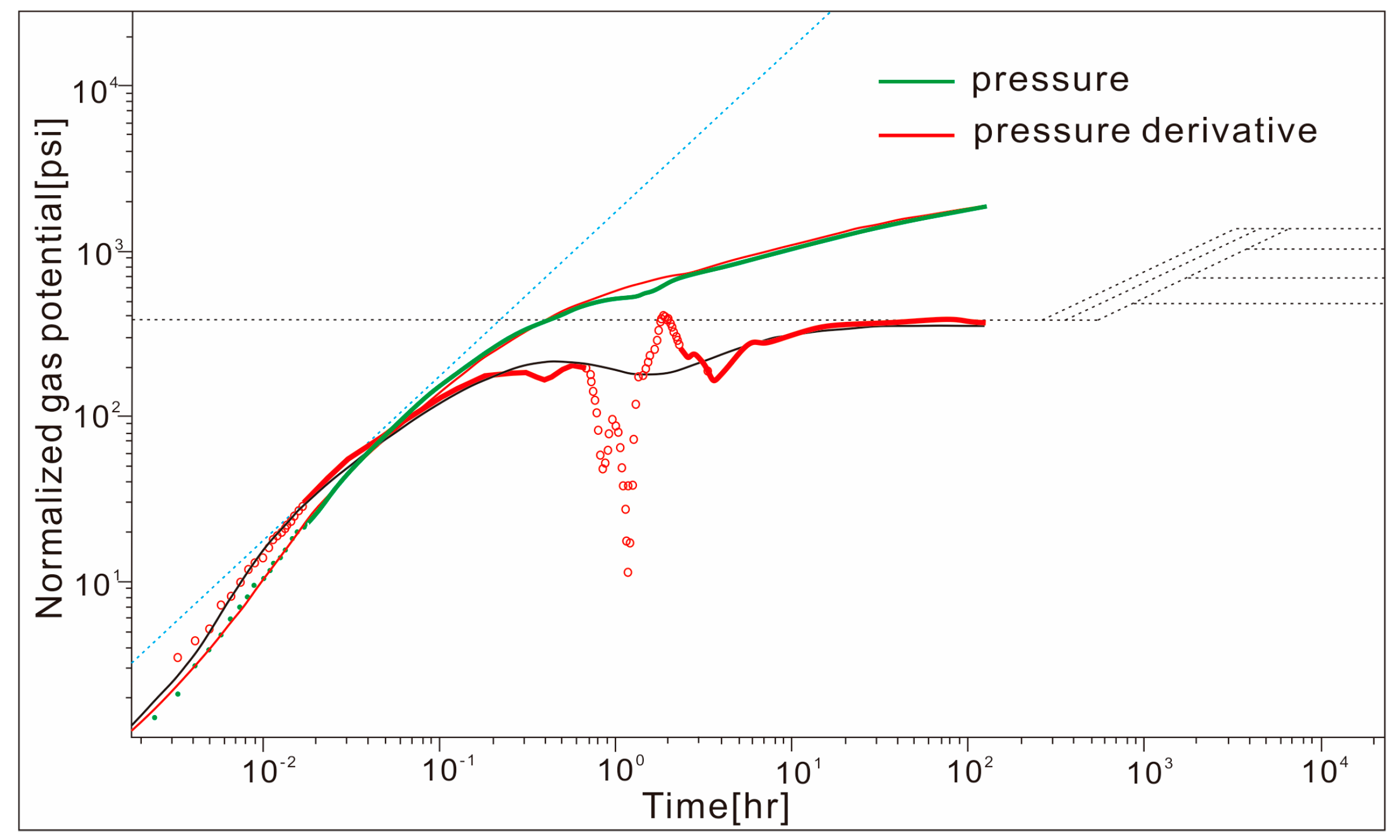
On account of the comprehensive analysis of the features of each stage of the pressure−recovery double logarithmic curve of Well A, the variable well reservoir + horizontal well + fracture + dual pore medium model was chosen to simulate the analysis of the pressure-recovery-test curve, and the pressure history fitting and double logarithmic fitting were completed (Figure 6). The interpretation results are shown in Table 1. The interpretation results showed that the formation coefficient was 1.014−2.734, the permeability was 0.023 mD−0.062 mD, and the low permeability reservoir, the reservoir, showed obvious double pore medium characteristics; in the double logarithmic fitting curve, due to the incomplete appearance of the later pseudo-radial flow section, the well-test interpretation could only determine the range of permeability and skin factor.

Figure 6.
Double logarithmic fitting result diagram of Well A.

Table 1.
Well−test interpretation result table of Well A.
Based on the well−test interpretation of the selected variable well storage + horizontal well + dual porosity medium model, using the Blasingame modern production-decline analysis method, two models of horizontal fracture + dual porosity medium + circular boundary and horizontal radial + dual porosity medium + circular boundary were established to fit and analyze the production dynamics data of Well A. The fitting charts are shown in Figure 7 and Figure 8.
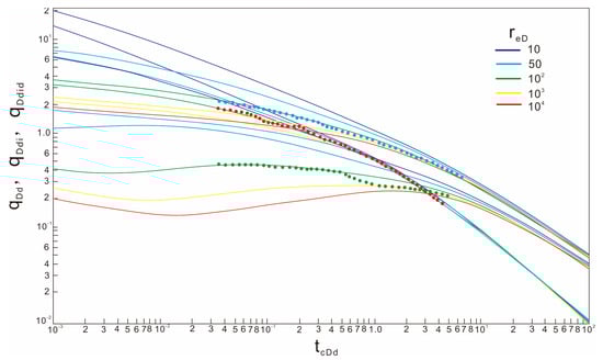
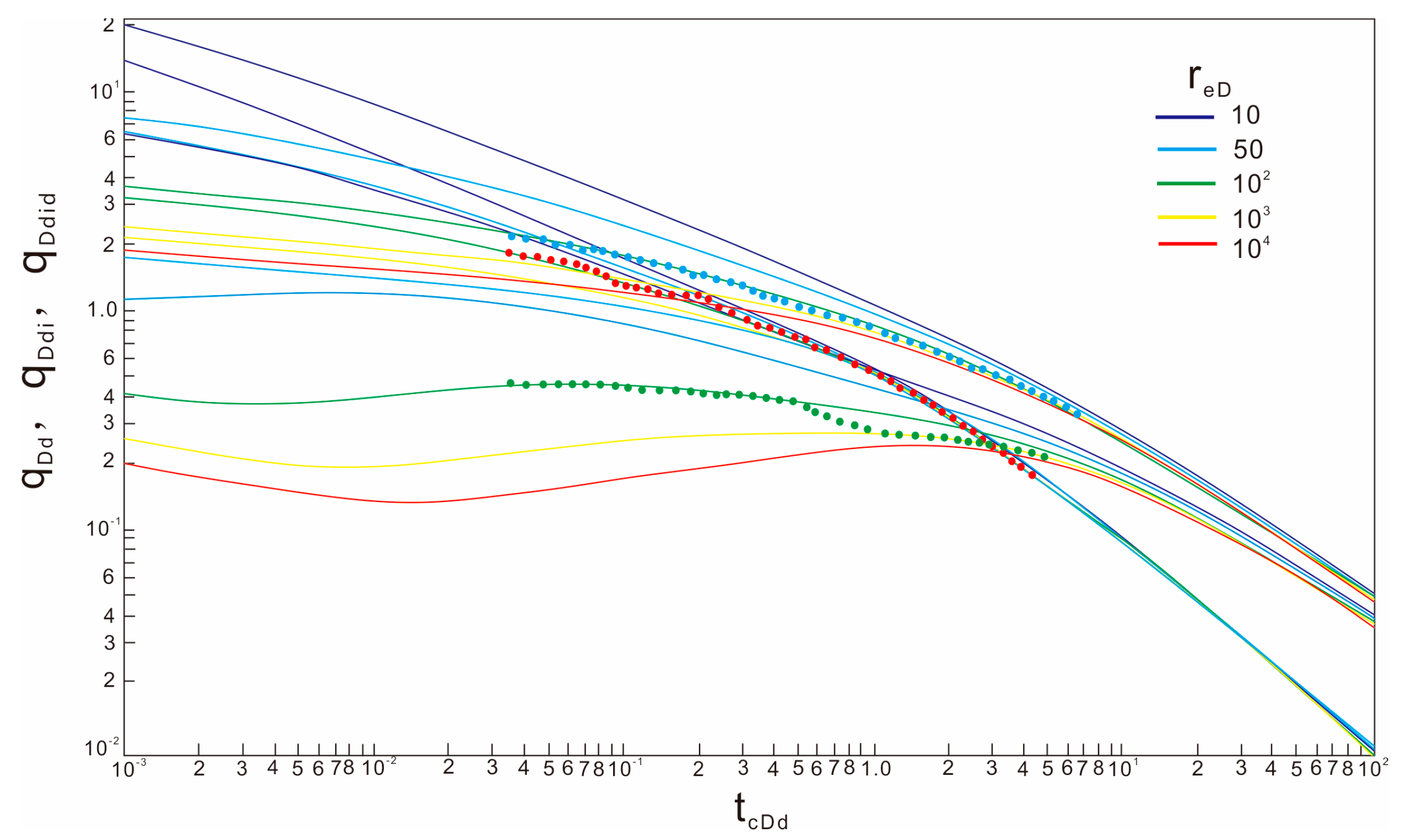
Figure 7.
Well A Model 1 production dynamics data fitting diagram. The round point represents the dimensionless yield, the dimensionless yield integral, the dimensionless yield integral derivative corresponding to different time, and the red point is the dimensionless yield. The blue point is no yield integral; the green point is the dimensionless yield integral derivative.
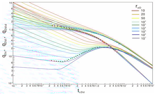
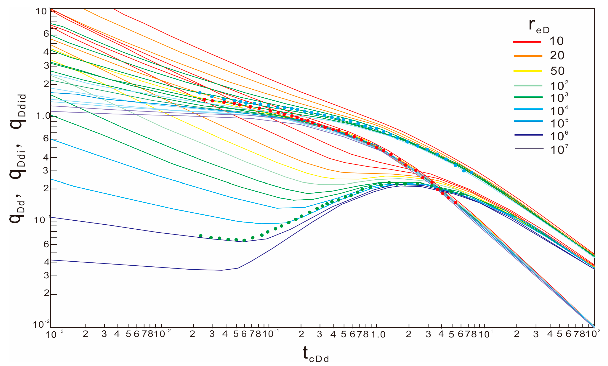
Figure 8.
Well A Model 2 production dynamics data fitting diagram. The round point represents the dimensionless yield, the dimensionless yield integral, the dimensionless yield integral derivative corresponding to different time, and the red point is the dimensionless yield. The blue point is no yield integral; the green point is the dimensionless yield integral derivative.
From the production dynamics data fitting diagram of Well A Model 1, it can be seen that the well had the characteristics of a dual pore medium in the later stage. The results calculated by fitting analysis were as follows: permeability was 0.0297 mD, well control radius was 245.8 m, skin factor was −2.44, and dynamic reserves were 1.197 × 10⁸ m3. The permeability of the well was low, the dynamic reserves were small, and the reservoir had low porosity and low permeability.
From the production dynamics data fitting diagram of Well A Model 2, it can be seen that the well had the characteristics of a dual pore medium in the later stage. The results calculated by fitting analysis were as follows: permeability was 0.0335 mD, well control radius was 261.1 m, skin factor was −2.26, and dynamic reserves were 1.224 × 10⁸ m3. The permeability of the well was low, the dynamic reserves were small, and the reservoir had low porosity and low permeability.
Comparing the results obtained by the Blasingame method with the results obtained by several other modern production−decline analysis methods, from the comparison table of the interpretation parameters of each method (Table 2), it can be seen that the skin factor, well control radius, and well control reserve values calculated by these modern production−decline methods were basically the same. In terms of permeability, due to the short period of the pressure-recovery well test, the influence range of pressure fluctuation was small, while the production data time span used in the modern production−decline analysis method was longer, and the influence range of pressure fluctuation was larger. Therefore, the calculation results of the pressure−recovery well test were different to those of the modern production−decline analysis method. In general, several methods can reflect the formation characteristics and can be verified by each other.
Table 2.
Comparison table of interpretation parameters of each method.
At the same time, we calculated the error of well−controlled reserves obtained by various modern production-decline analysis methods. The standard error of well−controlled reserves was 2.6952%, and the result was less than 5%. Therefore, it can be seen that Blasingame analysis results for condensate gas reservoirs have high accuracy and can interpret and analyze condensate gas reservoirs well.
5. Conclusions
- (1)
- The modern production-decline method of Blasingame introduces the equivalent time and pseudo-time of material balance and draws the curve of the production function and material balance time. The typical chart-fitting analysis method was used to calculate the permeability, well control radius, skin factor, well control reserves, and other parameters, which significantly improved the estimation accuracy of dynamic reserves of buried hill condensate gas reservoirs.
- (2)
- The model obtained by well-test interpretation was used to establish a more accurate Blasingame modern production-decline analysis model, and the reservoir physical property evaluation and reserve calculation were realized after fitting with the production dynamics data. Compared with the pressure-recovery unstable-well test method, it has the advantages of low cost, small operation volume, and accurate calculation parameters and can obtain the single well control boundary.
- (3)
- Well A was a low porosity and low permeability reservoir with a permeability of 0.0316 mD, a skin factor of −2.35, a well control radius of 253.5 m, and dynamic reserves of 1.211 × 10⁸ m3.
Author Contributions
Conceptualization, L.L. and P.C.; methodology, L.L.; software, L.L.; validation, L.L., P.C., and H.L.; formal analysis, L.L.; investigation, L.L.; resources, P.C.; data curation, H.L.; writing—original draft preparation, L.L.; writing—review and editing, P.C.; visualization, L.L.; supervision, H.L.; project administration, H.L. All authors have read and agreed to the published version of the manuscript.
Funding
This research received no external funding.
Data Availability Statement
The original contributions presented in this study are included in the article. Further inquiries can be directed to the corresponding author.
Conflicts of Interest
The authors declare no conflicts of interest.
Abbreviations
The following abbreviations are used in this manuscript:
| qD | The output solution of constant pressure production; |
| tcD | Dimensionless material equilibrium time; |
| tD | Dimensionless time; |
| pD | Dimensionless production; |
| μ | Fluid viscosity; |
| Z | Gas compressibility factor; |
| tca | Material balance pseudo-time; |
| Ct | Composite compressibility; |
| p | Pressure (MPa); |
| q | Daily production (104 m3/d); |
| K | Permeability (mD); |
| s | Skin coefficient; |
| re | Well control radius (m); |
| G | Original geological reserves (108 m3); |
| pi | Original formation pressure (MPa); |
| pp | Regularized pseudo-pressure; |
| pwf | Bottom hole flowing pressure (MPa); |
| B | Volumetric coefficient; |
| h | Strata thickness (m); |
| Φ | Formation porosity; |
| reD | Dimensionless well control radius; |
| rw | Wellbore radius (m); |
| rwa | Effective wellbore radius (m); |
| i | Integral; |
| D | Differential coefficient. |
References
- Li, S.; Sun, L.; Du, J.; Tang, Y.; Zhou, S.; Guo, P.; Liu, J. Difficulties and countermeasures in the development of low permeability tight gas reservoirs and condensate gas reservoirs. Xinjiang Pet. Geol. 2004, 25, 156–159. [Google Scholar]
- China Petroleum Exploration and Production Branch. Natural Gas Exploration and Development Technology Papers; Petroleum Industry Press: Beijing, China, 2000; pp. 7–127. [Google Scholar]
- Anderson, D.M.; Stotts, G.W.; Mattar, L.; Ilk, D.; Blasingame, T.A. Production data analysis challenges, pitfalls, diagnostics. In Proceedings of the SPE Annual Technical Conference and Exhibition, San Antonio, TX, USA, 24–27 September 2006; SPE 102048. [Google Scholar]
- Borch, C. Applied Multisource Pressure Data Integration for Dynamic Reservoir Characterization, Reservoir, and Production Management: A Case History from the SiriField, Offshore Denmark. In Proceedings of the SPE Annual Technical Conference and Exhibition, New Orleans, LA, USA, 30 September–3 October 2001; SPE 71629. [Google Scholar]
- Ma, C.; Wu, Y.; Liang, S.; Yang, H. Single well dynamic description of carbonate condensate gas reservoir. Inn. Mong. Petrochem. 2014, 40, 49–50. [Google Scholar]
- Guo, P.; Li, S.; Du, Z.; Sun, L.; Sun, L.; Li, M. Present Situation and Problems of Condensate Gas Reservoir Development Technology. Xinjiang Pet. Geol. 2002, 23, 262–264. [Google Scholar]
- Fraim, M.J. Gas reservoir decline—Curve analysis using type curves with real gas pseudo pressure and normalized time. SPE Form. Eval. 1989, 2, 671–682. [Google Scholar] [CrossRef]
- Hu, Y.; Li, M.; Wu, M. A simple method for production decline analysis of gas wells in low permeability gas reservoirs. Pet. Explor. Dev. 1999, 26, 60–62. [Google Scholar]
- Xu, L. Study on the Production Decline Analysis Method of Multi—Well Waterflooding Reservoir. Master’s Thesis, Xi’an University of Petroleum, Xi’an, China, 2013. [Google Scholar]
- Cao, Y. Application of Modern Production Decline Method in Pre-Fracturing Evaluation of Repeated Fracturing. Master’s Thesis, Chengdu University of Technology, Chengdu, China, 2016. [Google Scholar]
- Mattar, L.; Anderson, D.M. A Systematic and Comprehensive Methodology for Advanced Analysis of Production Data. In Proceedings of the SPE Annual Technical Conference and Exhibition, Denver, CO, USA, 5–8 October 2003; SPE 84472. [Google Scholar]
- Ahmed, T.; McKinney, P. Advanced Reservoir Engineering; Gulf Professional Publishing: Houston, TX, USA, 2011. [Google Scholar]
- Xie, W. Dynamic Analysis of Gas Well Production in Low Permeability Gas Reservoir. Master’s Thesis, Daqing Petroleum Institute: Daqing, China, 2009. [Google Scholar]
- Kabir, C.S.; Izgec, B. Diagnosis of Reservoir Behavior From Measured Pressure/Rate date. In Proceedings of the SPE Annual Technical Conference and Exhibition, San Antonio, TX, USA, 24–27 September 2006; SPE 100384. [Google Scholar]
- Hager, C.J.; Jones, J.R. Analyzing Flowing Production Data with Standard Pressure Transient Methods. In Proceedings of the SPE Rocky Mountain Petroleum Technology Conference, Keystone, CO, USA, 21–23 May 2001; SPE 71033. [Google Scholar]
- Zuo, Q. Dynamic Analysis of Gas Well Production in Water Gas Reservoir. Master’s Thesis, Southwest Petroleum University, Chengdu, China, 2018. [Google Scholar]
- Chen, J.; Wei, M.; Duan, Y. comparative analysis of different gas well production dynamic analysis methods. Nat. Gas Explor. Dev. 2012, 35, 56–59. [Google Scholar]
- Xu, X.; Mei, Q.; Chen, Y.; Han, Y.; Tang, H.; Jiao, C.; Guo, C. Comprehensive analysis method of gas reservoir water invasion and development dynamic experiment. Nat. Gas Geosci. 2020, 31, 1355–1366. [Google Scholar]
- Blasingame, T.A.; Johnston, J.L.; Lee, W.J. Type—Curve Analysis Using the Pressure Integral Method. In Proceedings of the SPE California Regional Meeting, Bakersfield, CA, USA, 5–7 April 1989; SPE 18799-MS. [Google Scholar]
- Yang, M.; Yu, Y.; Ma, D.; He, F. Condensate gas well productivity prediction method research. In Proceedings of the 2015 International Conference on Oil and Gas Field Exploration and Development, Xi’an, China, 20 September 2015; pp. 280–287. [Google Scholar]
- Yan, T.; Li, J. Determination of reasonable productivity of condensate gas wells in the East China Sea. Ocean. Oil 2007, 27, 70–76. [Google Scholar]
- Wang, Z.; Yao, J.; Wu, M. A New Well Test Interpretation Method for Fractured Condensate Gas Reservoirs. China Foreign Energy 2007, 12, 37–42. [Google Scholar]
- Jones, J.R.; Raghavan, R. Interpretation of Flowing Well Response in Gas-Condensate Wells. SPE Form Eval 1988, 3, 578–594. [Google Scholar] [CrossRef]
- Mazlcom, J.; Kelly, R.T.; Mahani, H. A New Two—Phase Pseudo Pressure Approach for the Interpretation of Gas Condensate Well Test in the Naturally Fractured Reservoir. In Proceedings of the SPE Europec/EAGE Annual Conference, Madrid, Spain, 13–16 June 2005; SPE 94189. [Google Scholar]
- Yang, Y.; Ou, J.; Li, J.; Xu, Q.; Lu, Y. A calculation method of gas well productivity based on production performance analysis. In Proceedings of the 33rd National Natural Gas Academic Annual Conference (2023) Proceedings (02 Gas Reservoir Development), Nanning, China, 31 May–2 June 2023; pp. 290–297. [Google Scholar]
- Sun, H.; Zhu, Z.; Shi, Y.; Yang, L.; Jiang, J. Error correction of Blasingame plate making in modern production decline analysis. Nat. Gas Ind. 2015, 35, 71–77. [Google Scholar]
- Palacio, J.C.; Blasingame, T.A. Decline curve analysis using type curves—Analysis of gas well production data. In Proceedings of the SPE Joint Rocky Mountain Regional and Low Permeability Reservoirs Symposium, Denver, CO, USA, 26–28 April 1993; SPE 25909. [Google Scholar]
- Liu, X.; Zou, C.; Jiang, Y.; Yang, X. Basic Principles and Applications of Modern Production Decline Analysis. Nat. Gas Ind. 2010, 30, 50–54+139–140. [Google Scholar]
- Liu, X. Discussion on several key parameters in the calculation of dynamic reserves of gas reservoirs. Nat. Gas Ind. 2009, 29, 71–74. [Google Scholar]
- Poston, S.W.; Poe, B.D., Jr. Analysis of Production Decline Curves; Society of Petroleum Engineers: Richardson, TX, USA, 2008. [Google Scholar]
- Li, X.; Cheng, Y.; Wang, R.; Cao, P.; Chang, S.; Liu, Y. Discussion on the application of the Blasingame production decline analysis method in the Sudong block. In Proceedings of the 14th Ningxia Young Scientists Forum Petrochemical Thematic, Yinchuan, China, 24 July 2018; Petrochemical Applications; pp. 463–464. [Google Scholar]
- Zareenjad, M.H.; Ghanavati, M.; Asl, A.K. Production data analysis of horizontal wells using vertical well decline models, a field case study of an oil field. Pet. Sci. Technol. 2014, 32, 418–425. [Google Scholar] [CrossRef]
- Nobakht, M.; Clarison, C.R.; Kaviani, D. New type curves for analyzing horizontal wells with multiple fractures in shale gas reservoirs. J. Nat. Gas Sci. Eng. 2013, 10, 99–112. [Google Scholar] [CrossRef]
- Ali, A.J.; Siddiqui, S.; Dehghanpour, H. Analyzing the production data of fractured horizontal wells by a linear triple porosity model: Development of analysis equations. J. Pet. Sci. Eng. 2013, 112, 117–128. [Google Scholar] [CrossRef]
- Hui, G.; Chen, Z.; Wang, Y.; Zhang, D.; Gu, F. An Integrated Machine Learning-Based Approach to Identifying Controlling Factors of Unconventional Shale Productivity. Energy 2023, 266, 126512. [Google Scholar] [CrossRef]
- Bai, W.; Cheng, S.; Wang, Y.; Cai, D.; Guo, X.; Guo, Q. A transient production prediction method for tight condensate gas wells with multiphase flow. Pet. Explor. Dev. 2024, 51, 1–7. [Google Scholar] [CrossRef]
- Han, J.; Wu, G.; Yang, H.; Dai, L.; Su, Z.; Tang, H.; Xiong, C. Type and genesis of condensate gas reservoir in the Tazhong uplift of the Tarim basin. Nat. Gas Ind. 2021, 41, 24–32. [Google Scholar]
- Du, P. Study on Mechanism of Enhanced Oil Recovery by Gas Injection in the Middle and Late Phases of Condensate Gas Reservoir with High Condensate Oil Content Development. Master’s Thesis, Southwest Petroleum University, Chengdu, China, 2018. [Google Scholar]
- Fevang, Ø.; Whitson, C.H. Modeling gas-condensate well deliverability. SPE Reserv. Eng. 1996, 11, 221–230. [Google Scholar] [CrossRef]
- Liu, X.; Zou, C.; Jiang, Y.; Yang, X. Theory and application of modern production decline analysis. Nat. Gas Ind. 2010, 30, 50–54. [Google Scholar]
- Jiang, R.; He, J.; Jiang, Y.; Fan, H. Establishment and application of Blasingame production decline analysis method for fractured horizontal well in shale gas reservoirs. Acta Pet. Sin. 2019, 40, 1503–1510. [Google Scholar]
- Guo, P.; Ou, Z. Material balance equation of a condensate gas reservoir considering water soluble gas. Nat. Gas Ind. 2013, 33, 70–74. [Google Scholar]
- Chen, Y.; Ma, F.; Wang, X.; Li, J.; Jiang, H. New calculation method of material equilibrium equation for condensate reservoirs. Nat. Gas Ind. 2005, 25, 104–106. [Google Scholar]
- Wang, J.; Guo, P.; Wang, F.; Liang, C.; Bo, Z. Calculation of dynamic reserves in fracture-cavity gas condensate reservoirs with material balance method. Spec. Oil Gas Reserv. 2015, 22, 75–77. [Google Scholar]

Disclaimer/Publisher’s Note: The statements, opinions and data contained in all publications are solely those of the individual author(s) and contributor(s) and not of MDPI and/or the editor(s). MDPI and/or the editor(s) disclaim responsibility for any injury to people or property resulting from any ideas, methods, instructions or products referred to in the content. |
© 2025 by the authors. Licensee MDPI, Basel, Switzerland. This article is an open access article distributed under the terms and conditions of the Creative Commons Attribution (CC BY) license (https://creativecommons.org/licenses/by/4.0/).